HAL Id: hal-01361432
https://hal.sorbonne-universite.fr/hal-01361432
Submitted on 7 Sep 2016
HAL is a multi-disciplinary open access
archive for the deposit and dissemination of
sci-entific research documents, whether they are
pub-lished or not. The documents may come from
teaching and research institutions in France or
abroad, or from public or private research centers.
L’archive ouverte pluridisciplinaire HAL, est
destinée au dépôt et à la diffusion de documents
scientifiques de niveau recherche, publiés ou non,
émanant des établissements d’enseignement et de
recherche français ou étrangers, des laboratoires
publics ou privés.
Distributed under a Creative Commons Attribution| 4.0 International License
T. Stavrakou, J.-F. Müller, M. Bauwens, I. de Smedt, C. Lerot, et al.. Substantial
Underestima-tion of Post-Harvest Burning Emissions in the North China Plain Revealed by Multi-Species Space
Observations. Scientific Reports, Nature Publishing Group, 2016, 6, pp.32307. �10.1038/srep32307�.
�hal-01361432�
Substantial Underestimation of
Post-Harvest Burning Emissions in
the North China Plain Revealed by
Multi-Species Space Observations
T. Stavrakou
1, J.-F. Müller
1, M. Bauwens
1, I. De Smedt
1, C. Lerot
1, M. Van Roozendael
1,
P.-F. Coheur
2, C. Clerbaux
2,3, K. F. Boersma
4,5, R. van der A
4& Y. Song
6The large-scale burning of crop residues in the North China Plain (NCP), one of the most densely populated world regions, was recently recognized to cause severe air pollution and harmful health effects. A reliable quantification of the magnitude of these fires is needed to assess regional air quality. Here, we use an eight-year record (2005–2012) of formaldehyde measurements from space to constrain the emissions of volatile organic compounds (VOCs) in this region. Using inverse modelling, we derive that satellite-based post-harvest burning fluxes are, on average, at least a factor of 2 higher than state-of-the-art bottom-up statistical estimates, although with significant interannual variability. Crop burning is calculated to cause important increases in surface ozone (+7%) and fine aerosol concentrations (+18%) in the North China Plain in June. The impact of crop fires is also found in satellite observations of other species, glyoxal, nitrogen dioxide and methanol, and we show that those measurements validate the magnitude of the top-down fluxes. Our study indicates that the top-down crop burning fluxes of VOCs in June exceed by almost a factor of 2 the combined emissions from other anthropogenic activities in this region, underscoring the need for targeted actions towards changes in agricultural management practices.
The North China Plain covers an area of approximately 400,000 km2, extending over the provinces of Hebei,
Shandong, Henan, Anhui, and Jiangsu. Thanks to its fertile soil, this region is one of the largest agricultural plains, and among the most densely populated areas of the world, home to over 300 million people. Wheat and maize are the two main crops in this area and their growth in rotation is a common practice in response to the increasing food demand1,2. The winter wheat growing season, between February and mid-May, is followed by
harvesting in early June, whereas maize grows in July-August and is harvested in September until mid-October3.
Large-scale agricultural burning during post-harvest season is a well-established practice which is repeated every year3. It helps field clearing and preparation for the next crop but has been recognized to cause extremely poor
air quality and raises concerns about adverse effects on human health4. Straw burning limitations are actively
debated in China but their implementation often faces the reluctance of farmers who use ash as a natural fertil-iser. Quantifying the magnitude of the associated emissions and their impact on regional air quality is therefore urgently needed.
Bottom-up inventories based exclusively on satellite fire products generally underestimate the agricultural fires because of their small burnt area and intermittency. As an example, the VOC emission in the NCP (defined here as the region bounded by 32–40°N and 112.5–120°E) is estimated at ca. 40 Gg in June according to GFED35,
a factor of 10 lower than a detailed bottom-up estimate based on province-level statistical data and satellite fire products for spatial allocation6. Statistical information is however not available for every year, and cannot be used
1Royal Belgian Institute for Space Aeronomy, Avenue Circulaire 3, 1180, Brussels, Belgium. 2Spectroscopie
de l’Atmosphère, Service de Chimie Quantique et Photophysique, Université Libre de Bruxelles (ULB), 1050, Belgium. 3LATMOS/IPSL, UPMC Univ. Paris 06 Sorbonne Universités, UVSQ, CNRS, Paris, France. 4Royal
Netherlands Meteorological Institute, De Bilt, The Netherlands. 5Wageningen University, Meteorology and Air
Quality department, Wageningen, The Netherlands. 6Department of Environmental Science, Peking University,
Beijing 100871, China. Correspondence and requests for materials should be addressed to T.S. (email: Trissevgeni. Stavrakou@aeronomie.be)
Received: 13 April 2016 Accepted: 14 July 2016 Published: 31 August 2016
to assess interannual variability or evaluate emission abatement measures. In addition, the bottom-up estimation based on such statistical information for this type of emission source carries large uncertainties.
Space-based remote sensing observations of atmospheric gases offer an alternative and independent way to constrain the crop fire fluxes. Formaldehyde (HCHO) columns retrieved from the GOME satellite measurements over 1996–2001 show a large systematic column enhancement in the NCP in June, spatially coinciding with the extent of fire activity in the region, suggesting that the bottom-up biomass burning estimates are strongly under-estimated in this region7. Latest generation satellite sounders with high signal-to-noise ratio and daily global
coverage, such as the Ozone Monitoring Instrument (OMI), launched aboard the Aura platform in 20048, as
well as recent advances in trace gas retrievals9–12 offer the capability to derive satellite-constrained estimates of
post-harvest burning emissions, to assess their year-to-year variability and to investigate their importance on regional air quality. To reach this objective, we use vertical columns of HCHO retrieved by OMI10 for all years
between 2005 and 2012 to constrain the monthly emissions of HCHO precursors from fire burning, anthropo-genic activities and vegetation. The emissions are optimised by inverse modelling of satellite HCHO columns performed using the adjoint of the IMAGESv2 chemistry-transport model13–15 (cf. Methods). The OMI-based a
posteriori post-harvest emissions are evaluated against vertical columns of HCHO retrieved from the GOME-2 satellite sensor, and are compared with independent bottom-up inventories. Finally, analysis of glyoxal and NO2
column observations by OMI, and methanol column observations from the Infrared Atmospheric Sounding Interferometer (IASI) confirms the detection of crop burning from space and corroborates the top-down fluxes.
Results
Top-down agricultural fire emissions.
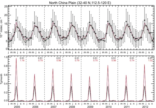
The OMI observations reveal enhanced formaldehyde columns in June in the NCP for all years of the study period, as illustrated in Figs 1–3. The observed columns are higher in June than in the adjacent months, by about 50% and 15% compared to May and July, respectively, pointing to the significant source from agricultural burning alongside the anthropogenic and biogenic sources of this region. The seasonal cycle of the observed HCHO columns exhibits a large amplitude with a minimum in win-ter (6–7 × 10¹⁵ molec.cm−2) and maximum in summer (12–17 × 1015 molec.cm−2), and in particular in June(15–17 × 1015 molec.cm−2). This variability is mostly due to the higher photochemical activity in summertime, as the
biogenic isoprene emissions are shown to be very small for croplands16. In winter, formaldehyde production from
anthropogenic hydrocarbon oxidation is diluted, due to slower oxidation rates associated to low solar radiation. The a priori model simulation reproduces well the seasonal cycle of formaldehyde (Fig. 3(a)), except in winter and in June, when the model persistently underestimates the observations by about 30% and 16%, respectively.
The optimisation setup adopted to infer VOC fluxes minimising the model-observation mismatch, uses satel-lite columns observed over a complete year. The top-down fluxes from all emission categories are derived simulta-neously. Although the emission inversions were conducted at 2° × 2.5° resolution, we also used a regional version of the same model running at 0.5° × 0.5° to verify that resolution has only a limited impact on average modelled HCHO columns in this region, in spite of the non-linearity in tropospheric chemistry and the strong spatial het-erogeneity of emissions (Fig. S1).
The optimisation leads to a substantial increase of the agricultural waste burning source in June, by a factor of 2 on average for 2005–2012 with respect to the a priori inventory6. The top-down mean annual flux is estimated
at 900 Gg, i.e. 76% higher than the a priori estimate (510 GgVOC, Fig. 3(b)). This increase improves consider-ably the agreement with the observations in June (Fig. 3(a)), reducing the mean discrepancy from 16% in the a priori to 6% in the a posteriori (OMI: 16.2 × 10¹⁵ molec.cm−2, a priori model: 13.9 × 10¹⁵ molec.cm−2, top-down:
15.3 × 10¹⁵ molec.cm−2), although for some years the optimised columns remain slightly underpredicted after
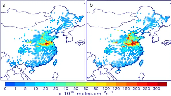
optimisation. The spatial distribution of the optimised biomass burning fluxes (Fig. 2) suggests the strongest enhancements (factor of 3) at the northernmost latitudes (> 36°N) and substantial increases (factor of 2.5)
Figure 1. HCHO columns in June averaged over 2005–2012 (in 1015 molec.cm−2). (a) Observed by OMI. (b) Simulated a priori model column. (c) A posteriori model column. The black box in (a) delimits the study area: 32–40°N, 112.5–120°E. The maps were generated with IDL version 8.2.3 software (http://www.exelisvis.com).
between 34°N and 36°N. Moderate emission increases (by 70%) are derived in the southern part of the NCP, which is the dominant emitting region6 (Table S1).
In order to provide a better match with OMI observations (Fig. 3(a)), anthropogenic VOC emissions are increased during the winter months by about 25% on average for all years, whereas in summertime, the observa-tions suggest a posterior decrease of the anthropogenic source, by about 10% in comparison to the a priori inven-tory (REASv2) in June (Fig. S2). The optimised anthropogenic fluxes during summer, approx. 470 Gg/month, are in excellent agreement with the independent flux estimate of 460 Gg/month from the Multi-Resolution Emission Inventory for China (MEIC)17. Contrary to earlier knowledge, the crop fire burning source of VOCs in the NCP
in June outweighs the combined emissions from all other human-related activities (power generation, industrial/ residential sector, transportation) by about a factor of two.
The errors on the a posteriori emissions are calculated by applying an off-line iterative approximation of the inverse Hessian matrix, as described in Methods. The error on the total pyrogenic NMVOC emissions in the NCP in June is lowered from a factor of 3.7 in the a priori to a factor of 1.8 after optimisation. For anthropogenic emis-sions, the reduction is considerably less important, from a factor of 1.45 (a priori) to a factor of 1.37 (optimised).
Impact on the atmospheric composition.
Post-harvest burning in June is estimated to have released on average 735 GgVOC (Table S1), as well as 2.1 TgCO, 25 GgNOx-N, and 0.1 TgC of carbonaceous aerosols, based on emission factor estimates for agricultural waste burning18. Note that the figure for NOx would be doubledif the emissions factor estimate from a recent compilation of measurements performed in fresh smoke19 were
used;in any case, this contribution remains minor in comparison with the anthropogenic emission fluxes in the NCP in June (180 GgNOx-N20).
To quantify the impact of these emissions on air pollution, we perform simulations for a specific year (2010) using the model in regional mode at 0.5° resolution (Fig. S3). Compared to a model simulation ignoring those emissions, the average near-surface ozone in the NCP is increased by 7%, with the largest increases (up to 20%) calculated in the south-central part of the region. The dominant cause of this increase is the large contribu-tion of crop fire emissions, 65% and 32%, to the total emissions of VOC and CO in the NCP, respectively. The observed seasonal variation of ozone in the NCP shows a clear maximum in June21–23, in agreement with the
model. Meteorological factors are believed to be its primary cause, with however a significant contribution of crop residue burning. The calculated values in June agree fairly well with observations e.g. at Mount Tai21, with 85 ppbv
observed vs. 70 ppbv in the model, and at Miyun22 (71 vs. 73 ppbv). Observations of lower tropospheric ozone by
IASI23 show a similar pattern, with 26–30 Dobson Units (DU) below 6 km altitude in June (32 DU in the model),
and lower values in May and July (28–29 DU in the model).
The calculated impact on near-surface CO and HCHO is important, + 25% and + 50% on average, respectively. The enhanced emissions lead to an overall decline of OH levels, between 5 and 25% within the boundary layer whereas HO2 levels increase by 10–18%, mainly due to conversion of OH to HO2 upon reaction with CO and
VOC. The calculated impact of agricultural fires on NOx concentrations is low (+ 1% on average), owing to the low NOx emission factors for agricultural fires18,19. Finally, in the presence of crop fires, the fine aerosol loadings are
increased by about 18% or ca. 10 μg m−3 compared to the values estimated without crop burning (30–60 μg m−3).
The calculated concentrations lie within the wide range of measured PM2.5 levels during spring in the NCP, e.g.
25 μg m−3 in Xianghe24 and 177 μg m−3 in Nankou25.
Figure 2. Post-harvest VOC burning fluxes in June expressed in 1010 molec.cm−2 s−1. (a) As estimated by the a priori inventory6. (b) Average over 2005–2012 constrained by the OMI observations. The maps were generated
Interannual emission variability.
The interannual variability of the observed columns in June is moderate with ca. 10% difference between the highest (2012) and lowest years (2006 and 2008) of the studied period (Fig. S4). The derived flux estimates, however, exhibit a much stronger interannual variability, the difference between the maximum and minimum top-down emission in June reaching ca. 50–70%. This apparent discrepancy is largely explained by the important contribution of other HCHO sources to the total column, including local anthropo-genic emissions (ca. 17%), isoprene (5%) and more importantly, the background production of HCHO due to oxidation of methane and other VOCs imported to the NCP from neighbouring regions, which we estimate to about 50% based on a sensitivity calculation. The strongest flux enhancements are found in 2005, 2010, and 2012, with increases from 350 GgVOC in the bottom-up inventory to 996, 831 and 850 GgVOC, respectively, while in 2008, 2009 and 2011 the emission increased by less than a factor of 2 compared to the a priori (Table S1).The lower crop burning fluxes in 2008 and 2009 are likely due to regulation measures aimed to ensure cleaner air conditions during the 2008 Beijing Olympics. Open field burning was banned in Northern China from May to September 200826, as demonstrated by the smaller number of MODIS fire counts (− 60%) in 2008 compared to
2007. The fire counts increased again gradually after 2009, and a maximum was observed in 2012 (Fig. S5). The lower observed HCHO columns and fire counts in June 2011 compared to 2010 and 2012 might be attributed to reduced crop yields due to a major drought event, not unusual in this region27. Indeed, ERA-Interim analyses28
show that the region received about twice lower rainfall beween January and May in 2011 compared to other studied years, which likely caused decreased crop yields and agricultural waste.
The top-down emissions, expressed as burnt biomass (in TgC), are compared with four independent inven-tories for biomass burning in Fig. S6. Two versions of the Global Fire Emissions Database are used, version 35
and the GFED4s which includes burned area from small fires based on active fire detections29; the Global Fire
Assimilation System (GFAS) based on assimilation of fire radiative power observed from MODIS aboard the Terra and Aqua satellites30, and the Fire Inventory from NCAR (FINN) version 1.5, an updated version of the
FINN inventory31. On average over the eight years the top-down emissions are about 14, 7 and 4 times larger than
in GFAS, GFED4s, and FINN, respectively, whereas the GFED3 emissions are even lower. In terms of interannual variability, the GFED4s and GFAS fluxes correlate better with the satellite-derived fluxes (r = 0.58) than the FINN emissions (r = 0.45). Finally, the updated fluxes over NCP in June are found to be well correlated spatially with the MODIS fire counts (r > 0.7 for most years). Their interannual variability is also very similar (Fig. S5), especially between 2006 and 2012 (r = 0.73).
Sensitivity inversions.
The uncertainty on the top-down source is evaluated by conducting sensitivity opti-misations to quantify the role of key parameteters, namely (i) the assigned a priori flux errors, (ii) the fire-related emission factors, (iii) the inversion setup, and (iv) the diurnal cycle of fire activity. Although this evaluation does not cover all possible sources of errors, it accounts for the most important uncertainties associated with the model and the inversion framework.Figure 3. Monthly HCHO columns and agricultural burning fluxes between 2005 and 2012 in the North China Plain. (a) Time series observed by OMI (black asterisks and error bars), a priori model (black solid line),
optimised (red). (b) A priori biomass burning emission fluxes (constant for all years, black), and optimised fluxes (red). Annual fluxes (in TgVOC) are shown inset using the same color code.
As not only the a priori emissions themselves but also their uncertainties are difficult to evaluate, the assigned errors on the a priori biomass burning emissions were doubled and halved in DE and HE optimisations (Table 1), respectively, with respect to the initially assigned error (cf. Methods). As expected, the DE inversion realises a stronger bias reduction, compared to the a priori, 70% vs. 56% in the standard (STD) optimisation. The better agreement with the observations is realised by even larger emissions, 950 Gg in DE vs. 850 Gg and 690 Gg in STD and HE, respectively. The increase is especially pronounced in the northernmost part of the NCP (ca. factor of 5), apparently reflecting a misrepresentation of the spatial patterns of the a priori emissions, for reasons currently unclear (Table 1, Fig. S7).
Another important source of uncertainty lies in the assumed biomass burning emission factors. The standard setup employs the widely used updated (2011) emission factors from ref. 18, whereas a recent compilation of emission factors based on measurements performed in fresh smoke19 is adopted in two sensitivity inversions, AK
and AKU. The agricultural waste emission factors are similar in both databases for most compounds, however large differences exist for individual compounds, e.g. acetaldehyde (2.77 g/kg in ref. 18, 1.24 in ref. 19), glyoxal and methylglyoxal (1.0 and 0.73 g/kg in ref. 18, 0 in ref. 19). Comparison with measurements of crop burning emission factors in China32 indicates that the emission factors adopted in our standard simulation18 are likely
too high for oxygenated compounds (as they are not corrected for chemical production in the fire plumes) and possibly too low for pure hydrocarbons such as alkanes, alkenes and aromatics. A large source of variability and uncertainty might lie in the complex influence of fuel moisture on the emission factors33. Overall, the a
priori biomass burning emission in June is by 20% lower when the newer datasets19,32 are used (280 vs. 350 Gg,
Table 1). The optimisation AKU, also based on ref. 19, acknowledges the fact that a significant mass fraction of the gas-phase VOC emitted by biomass burning is unidentified, as revealed by field and laboratory measurements34,35.
Therefore, AKU includes an additional non-methane VOC source in the model, of magnitude equal to the known source19, distributed as 50% propene and 50% monoterpene, in such a way that the resulting mix has a HCHO
mass yield similar to the overall mass yield of the known source. Due to their short lifetimes, these VOCs are oxi-dised closer to their emission source than the more long-lived identified VOCs. As a result, the VOC mix in AKU leads to higher HCHO levels directly above the emitting region compared to AK and the standard STD case. After optimisation, both AK and AKU inversions result in a similar a posteriori flux (ca. 750 Gg), yet a better agreement with the measurements is achieved in the AKU optimisation, i.e. significant reduction of the bias (Table 1, Fig. S7), due to the shorter lifetime and higher a priori emissions of HCHO precursors in this scenario. Note that in this case, the increase relative to the a priori is moderate (40%).
To evaluate the role of interferences associated with the optimisation of non-fire emissions, we perform an optimisation varying only the biomass burning source, while the anthropogenic and biogenic VOC source remain equal to the a priori (BB inversion, Table 1). This setup worsens the agreement with the observations (Table 1), whereas the inferred flux is by 20% lower (ca. 650 Gg) than for the standard inversion (850 Gg). Finally, to account for the uncertainty associated with the choice of the diurnal cycle profile for fire emissions, and since MODIS fire counts indicate that the diurnal cycle of fire activity over large croplands of central Eurasia is insignificant36,
we performed the optimisation NDC (no diurnal cycle) assuming no diurnal variation in agricultural fires. The resulting bias and root mean square deviation are very similar in comparison with the standard inversion and a slightly higher (+ 3%) a posteriori flux is estimated. Overall, the top-down emission estimates appear robust across the different sensitivity cases, and indicate a flux increment of at least a factor of two compared to the a priori inventory.
Discussion
The strong increase in the satellite-derived fluxes is further corroborated by satellite observations of HCHO retrieved by the GOME-2 sensor onboard Metop-A which measures HCHO columns daily with a morning over-pass time (9:30 local time). As in the case of OMI (afternoon overover-pass 13:30), the GOME-2 dataset indicates a pronounced maximum in the NCP in June, by ca. 10–50% higher than the preceding and following months. The GOME-2 peak is by about 10% lower than the corresponding maximum observed by OMI (Figs 3 and 4), the
Simulation RMSD RMSRE % Bias Flux Gg 1015 molec.cm−2 1015 molec.cm−2 A priori 3.40 19.8 3.05 350 STD 2.20 13.2 1.32 850 DE 1.82 11.1 0.90 950 HE 2.75 16.2 2.05 690 AK 2.36 14.1 1.49 750 AKU 2.03 12.2 0.91 780 BB 2.29 13.6 1.59 647 NDC 2.18 13.1 1.42 878
Table 1. Root mean square deviation (RMSD), root mean square relative error (RMSRE) and bias between the OMI HCHO columns and the model predictions before and after the sensitivity inversions over the study region in June 2012. STD: standard inversion; DE and HE: doubled or halved a prori flux errors; AK
emission factors from19; AKU: as AK with additional source to account for unidentified VOCs; BB: only
biomass burning fluxes are varied; NDC: no diurnal cycle of fires. Note that the a priori crop fire fluxes in AK, AKU inversions are equal to 280 and 560 Gg in June 2012, respectively.
difference being primarily due to the diurnal cycle of HCHO columns, which is mostly affected by the diurnal cycle of emissions, as well as by OH and solar radiation levels15. The current version of the GOME-2 data is briefly
described in Section 1 of the Supplement and in detail in ref. 10. As seen in Fig. 4 (Fig. S8), the GOME-2 col-umns strongly support the findings inferred from OMI observations. The initial model underprediction by about 10–15% in June disappears almost completely when the OMI-based emissions are used, except to some extent in 2011 and 2012, where the model remains too low, as was already the case with respect to OMI. A sensitivity inver-sion using GOME-2 observations as top-down constraints for 2012 leads to an a posteriori flux of 968 GgVOC, i.e. 14% higher than the estimated emissions using OMI observations (Table 1). The mean bias between the GOME-2 columns and the optimised model results (2.54 × 10¹⁴ molec.cm−2) is about factor of 2 lower than in the a priori
simulation, and the a posteriori root mean square deviation is reduced by 30%.
The effects of crop residue burning in the NCP are detected from space in the observations of glyoxal (CHOCHO) retrieved by the OMI instrument. Glyoxal is formed in the oxidation of VOCs released by the biosphere, fires and human activities. The total glyoxal source is believed to be predominantly secondary and biogenic in origin37,38. Current models, however, largely underestimate the observed glyoxal satellite columns
sug-gesting the existence of, as yet unknown, additional sources37. To our best knowledge, only 18% of the total glyoxal
budget is due to biomass burning (primary and secondary), but this contribution is more pronounced at regional scale, where it often prevails over other sources38. The monthly OMI glyoxal columns over the study region
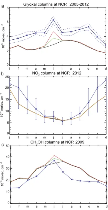
aver-aged over 2005–2012 are shown in Fig. 5a (Fig. S9). The retrieval algorithm, initially developed for GOME-2 observations12, was updated to account for the specifics of OMI (cf. Supplement, Section 2). The 2005–2012 June
mean observed glyoxal column in the NCP amounts to 6.3 × 10¹⁴ molec.cm−2, higher by 1.8 × 10¹⁴ molec.cm−2
than the mean value of May and July. A similar enhancement (1.5 × 10¹⁴ molec.cm−2) is derived by the model
when using the OMI-based optimised fluxes, whereas the a priori simulation strongly underestimated the peak (0.7 × 10¹⁴ molec.cm−2, Fig. 5a). Therefore, despite the model underprediction over the study region pointing to
missing glyoxal sources present all year long, the column enhancement due to post-harvest burning is well repro-duced by the model. This result lends confidence to the emission speciation profile, and in particular the glyoxal emission factor for agricultural fires (1.12 g/kg dry matter18), although this production might be largely due to
secondary formation due to fast oxidation of very short-lived, mostly unknown precursors. The secondary glyoxal peak observed in October (Fig. 5a), not reproduced by the a posteriori model, might be partly due to fires set up for clearing fields after the maize harvest season. These fires cause a secondary peak in the seasonal profile of the a priori emissions6, but of very weak amplitude, about a factor of 20 lower than the June peak. Furthermore, the
OMI HCHO dataset does not show a consistent pattern, with a local maximum in October seen only for two years (2006 and 2012) out of 8. Note that the higher zenith angles and lower magnitude of HCHO columns reduce the signal-to-noise ratio and the ability of the inversion to retrieve reliable fluxes in October.
The higher top-down emissions lead to a better agreement with satellite obeservations of NO2 from the OMI
instrument (DOMINOv211). The strong seasonal variation in the observed columns (Fig. 5b) is due to changes
in the chemical lifetime of NOx and is relatively well reproduced by the model. Since anthropogenic emissions are not expected to vary much between May and July, the observed column enhancement in June, relative to May and July is to a large extent due to pyrogenic emissions. Although relatively small, this enhancement (1.05 × 10¹⁵ molec.cm−2) is higher than predicted by the optimised model (0.27 × 10¹⁵ molec.cm−2, Fig. 5b). This
likely points to an underestimated NO2 emission factor for agricultural waste used in the model, 2.44 g per kg of
dry matter. Indeed, adopting the higher value (4.769 g/kg) suggested by19 and corroborated by an independent
study based on OMI NO2 measurements39, leads to a modelled enhancement of 0.97 × 10¹⁵ molec.cm−2, in very
good agreement with the observations.
Additional evidence for the intense burning in the NCP is given by methanol columns retrieved from the thermal infrared sensor IASI40 (cf. Supplement). Methanol is directly emitted by vegetation, anthropogenic
activ-ities, and open fires (55%, 5% and 3% of the global budget, respectively), whereas the remainder is due to oceanic emissions and secondary production41. In Fig. 5c the observed monthly averaged methanol columns in 2009 over
the NCP are compared with the model. The model overestimates the observations between June and September
Figure 4. Time series of monthly HCHO columns observed by GOME-2 (black asterisks and error bars) and from forward simulations neglecting crop fire fluxes (black), obtained from the a priori inventory6
(Fig. S9), likely due to an overestimation of biogenic emissions. However, use of the optimised emissions leads to a column enhancement in June of 6.3 × 10¹⁵ molec.cm−2, very close to the observed enhancement (7.7 × 10¹⁵ molec.
cm−2). Note that for methanol, the emission factors for agricultural burning are similar across recent
evalua-tions18,19,32 (between 2.94 and 3.45 g/kg, respectively).
Finally, it should be acknowledged that a significant source of error resides in the effects of aerosols in the UV-visible retrievals for individual observations above fire scenes7,42. This impact was, however, found to be
limited for monthly mean NO2 columns, suggesting that the effect of aerosols is reduced by spatiotemporal
averaging42, whereas accounting for an implicit or explicit aerosol correction leads to only a 6% difference in
the retrieved NO2 columns43. For fire scenes over Amazonia the impact of the aerosol correction was found to
only moderately affect the HCHO columns (3%), especially when aerosols are located throughout the boundary layer44, as is the case for crop residue burning. Furthermore, for weak absorbers like HCHO and CHOCHO,
errors on the vertical columns are as much due to slant column errors (calibration uncertainties, interferences with other species, etc.) as to errors in airmass factors.
Figure 5. Seasonal variability of (a) glyoxal, (b) NO2, and (c) CH3OH columns observed and modelled over
the North China Plain. Observations are shown in blue. Model results using crop fire fluxes set to zero, obtained from the a priori inventory6, and using the OMI-based estimates derived in this study are shown in black, green
and red, respectively. The dashed lines in (a) denote the standard deviation of the mean OMI glyoxal column over 2005–2012. The error bars in (b) represent the retrieval error of the DOMINOv2 dataset for the year 2012. The model NO2 column obtained using OMI-based fluxes and emission factors for agricultural waste burning
2005–2012 mean annual isoprene flux in China is estimated at 7.2 Tg, with the largest emission calculated in 2007 (7.6 Tg) and the lowest in 2012 (6.8 Tg).
The HCHO simulation is thoroughly described in refs 14,15. In the current version of the model, HCHO is formed in the oxidation of 24 explicit NMVOC precursors, namely, C2H2, C2H4, C2H6, C3H6, C3H8, isoprene,
α-pinene, HCHO, CH3CHO, glycolaldehyde, hydroxyacetone, methacrolein, methyl vinyl ketone, glyoxal,
methylglyoxal, methanol, formic acid, acetone, methyl ethyl ketone, biacetyl, acetic acid, benzene, toluene, and xylenes. Higher hydrocarbons are represented as a lumped compound with oxidation chemistry detailed in ref. 15. The speciation profile for pyrogenic emissions follows ref. 18 with 2011 updates. The average molecular weight of the mix of pyrogenic NMVOCs is equal to 46.7 kg kmol−1. The chemical mechanism uses molar yields
of glyoxal from benzene, toluene and xylenes of 75%, 70% and 36%, respectively47.
Satellite formaldehyde columns.
OMI (Ozone Monitoring Instrument), part of AURA’s payload launched in 2004, is a nadir-viewing UV-Visible sensor8 measuring global solar radiances backscattered fromthe Earth’s atmosphere daily in the early afternoon (ca. 13 h30 local time) at high spatial resolution (13 × 24 km2).
Slant column densities of HCHO are fitted in the 328.5–346 nm spectral window based on the algorithm described in ref. 9, which has been improved (i) to reduce the O2-O2 absorption effects and minimise the
inter-ferences with other molecules, (ii) to remove spike residuals, and (iii) to reduce offsets between rows by applying a destriping correction in the background reference sector10. These modifications eliminate inconsistencies and
unphysical results, increase the signal-to-noise ratio, and offer a higher temporal stability to the long-term dataset of OMI HCHO columns.
Monthly mean HCHO columns between 2005 and 2012 are used as constraints in a flux inversion scheme based on the discrete adjoint model of the IMAGESv2 global CTM (see below). The target region is Eastern China, and in particular the NCP delimited as 32–40°N, 112.5–120°E. Only observed columns with cloud frac-tion lower than 40% are used in the inversion. The error of the satellite columns is defined as the geometric mean of the retrieval error and an additional error of 2 × 10¹⁵ molec.cm−2. Error corelations between observations are
not considered. In the target region, the errors amounts to 45–48% in summertime, and up to 85% in winter. Monthly averaged columns with errors larger than 100% are not accounted for in the inversion. The model col-umns are sampled at the location and time of the observations. Column observations over oceans are excluded from the inversion analysis.
Inversion of surface fluxes.
This approach consists in minimising a scalar function (cost function) quan-tifying the mismatch between modelled and observed HCHO columns by adjusting the flux rates of the emit-ting sources on a monthly basis for every model grid13–15. The inversion is realised through the discrete adjointmethod, i.e. a line-by-line transpose of the tangent linear model in the reverse order, which consists in calculating the partial derivatives of the cost function
= − − − + −
J(f ) 1 H E H B
2[( (f ) y)T 1( (f ) y) fT 1f ], (1) with respect to emission parameters f to be optimised, where H(f) is the chemistry-transport model operating on the control variables, y is the observation operator, and E, and B are the covariance matrices of the errors on the observations and the emission parameters f, respectively, and T denotes the transpose of the vector. This
frame-work has been applied for inverting the fluxes of several atmospheric gases13,48,49, and is particularly appropriate
for reactive compounds, as it can account for chemical feedbacks. A priori emission distributions for anthropo-genic, pyrogenic and biogenic fluxes obtained from the latest available inventories are used in the model and are updated based on the satellite columns of formaldehyde through an iterative minimisation algorithm using the forward and its backward in time (adjoint) model. Of the order of 4 × 10¹⁴ emission parameters (of which 350 in
NCP) from all categories are optimised annually for every month and per grid cell with non-zero initial emission, and the minimum is achieved once the convergence criterion, set as a reduction of the norm of the cost function gradient by a factor of 103, is satisfied. The number of iterations required to achieve convergence varies from year
to year depending on the availability and errors of top-down constraints and generally lies between 30 and 50.
Inversion setups.
Annual inversions have been carried out between 2005 and 2012 using monthly HCHO columns, and VOC fluxes from anthropogenic, biomass burning and isoprene are updated on the global scale.The errors on the emission parameters, i.e. the diagonal elements of the matrix B, are assumed to be a factor of 2, 2.5, and 3 for anthropogenic, biogenic, and fire emissions, respectively. A larger error for the pyrogenic source is assumed over the NCP (factor of 7) to account for the large uncertainties and variability of this source. The off-diagonal elements of B represent spatiotemporal correlations between the errors of the emisssion parame-ters14,15. In our inversion experiments, the spatial terms are as in ref. 14, whereas the temporal terms decrease
linearly from 0.2 (for successive months) to zero (for a 6-month lag) for the biogenic and pyrogenic fluxes, and from 0.92 to 0.6 for the anthropogenic fluxes. No interannual correlations are assumed. Finally, the matrix E is assumed diagonal, and the errors on OMI HCHO columns are defined as previously.
Calculation of the a posteriori errors.
The posterior error covariance matrix of the control variables is defined as the inverse Hessian matrix of the cost function at its minimum. Assuming that the model is linear or weakly non-linear, the a posteriori error covariance matrix is related to the Hessian of the cost function J through the expression13:= H − H + − − =
Bpost [(D )TfE D1( )f B 1 1] ( ) ,IHf (2)
where ( )IHf =Hessian( )J−f1 is the inverse Hessian matrix calculated at the point f, DH is the Jacobian matrix of
the model, and E and B are as in Eq. (1). To calculate the inverse Hessian matrix we apply the Davidon-Fletcher- Powell (DFP) iterative approximation50, which uses the updated information obtained at each step k of the
minimisation: = + − + s s y s y y y y IH IH IH IH IH ( ) ( ) ( ) ( ) ( ) , (3) k k k k T kT k k k kT k kT k k 1
where =sk fk+1−fk, = ∇yk ( )J fk+1− ∇( )J fk, ∇J( )fk is the gradient of J at the point fk, and the initial inverse
Hessian matrix is taken to be equal to B. The approximate inverse Hessian matrix is then obtained through recur-sive application of the DFP updating formula on the vectors fk and ∇J( )fk calculated after each iteration. The
standard errors of the a posteriori variables f are the square roots of the diagonal elements of the inverse Hessian matrix, and the error reduction is defined as the ratio of the a priori to the a posteriori error.
References
1. National Bureau of Statistics of China. China Statistical Year Book 1995–2010, China Statistics Press (2010).
2. Jeong, S.-J. et al. Effects of double cropping on summer climate of the North China Plain and neighbouring regions. Nature Climate
Change 4, 615–619 (2014).
3. Huang, X., Song, Y., Li, M., Li, J. & Zhu, T. Harvest season, high polluted season in East China. Environ. Res. Lett. 7, 044033 (2012). 4. Yamaji, K. et al. Impact of open crop residual burning on air quality over Central Eastern China during the Mount Tai Experiment
2006 (MTX2006). Atmos. Chem. Phys. 10, 7353–7368 (2010).
5. van der Werf, G. R. et al. Global fire emissions and the contribution of deforestation, savanna, forest, agricultural, and peat fires (1997–2009). Atmos. Chem. Phys. 10, 11707–11735 (2010).
6. Huang, X., Li, M., Li, J. & Song, Y. A high-resolution emission inventory of crop burning in fields in China based on MODIS Thermal Anomalies/Fire products. Atmos. Environ. 50, 9–15 (2012).
7. Fu, T.-M. et al. Space-based formaldehyde measurements as constraints on volatile organic compound emissions in East and South Asia. J. Geophys. Res. 112, D6, doi: 10.1029/2006JD00785 (2007).
8. Levelt, P. F. et al. The Ozone Monitoring Instrument. IEEE T. Geosci. Remote Sens. 44, 1093–1101 (2006).
9. De Smedt, I. et al. Improved retrieval of global tropospheric formaldehyde columns from GOME-2/MetOp-A addressing noise reduction and instrumental degradation issues. Atmos. Meas. Tech. 5, 2933–2949 (2012).
10. De Smedt, I. et al. Diurnal, seasonal and long-term variations of global formaldehyde columns inferred from combined OMI and GOME-2 observations. Atmos. Chem. Phys. 15, 12519–12545 (2015).
11. Boersma, K. F. et al. An improved tropospheric NO2 column retrieval algorithm for the Ozone Monitoring Instrument. Atmos. Meas. Tech. 4, 1905–1928 (2011).
12. Lerot, C. et al. Glyoxal vertical columns from GOME-2 backscattered light measurements and comparisons with a global model.
Atmos. Chem. Phys. 10, 12059–12072 (2010).
13. Müller, J.-F. & Stavrakou, T. Inversion of CO and NOx emissions using the adjoint of the IMAGES model. Atmos. Chem. Phys. 5, 1157–1186 (2005).
14. Stavrakou, T., Müller, J.-F., De Smedt, I., Van Roozendael, M., van der Werf, G., Giglio, L. & Guenther, A. Global emissions of non-methane hydrocarbons deduced from SCIAMACHY formaldehyde columns through 2003–2006. Atmos. Chem. Phys. 9, 3663–3679 (2009).
15. Stavrakou, T. et al. How consistent are top-down hydrocarbon emissions based on formaldehyde observations from GOME-2 and OMI sensors? Atmos. Chem. Phys. 15, 12007–12067, doi: 10.5194/acpd-15-12007-2015 (2015).
16. Guenther, A., Karl, T., Harley, P., Wiedinmyer, C. Palmer, P. I. & Geron, C. Estimates of global terrestrial isoprene emissions using MEGAN (Model of Emissions of Gases and Aerosols from Nature). Atmos. Chem. Phys. 6, 3181–3210 (2006).
17. Li, M. et al. Mapping Asian anthropogenic emissions of non-methane volatile organic compounds to multiple chemical mechanisms.
Atmos. Chem. Phys. 14, 5617–5638 (2014).
18. Andreae, M. O. & Merlet, P. Emission of trace gases and aerosols from biomass burning. Global Biogeochem. Cy. 15, 955–966 (2001). 19. Akagi, S. et al. Emission factors for open and domestic biomass burning for use in atmospheric models. Atmos. Chem. Phys. 11,
4039–4072 (2011).
20. Kurokawa, J. et al. Emissions of air pollutants and greenhouse gases over Asian regions during 2000–2008: Regional Emission inventory in ASia (REAS) version 2. Atmos. Chem. Phys. 13, 11019–11058 (2013).
21. Sun, L. et al. Significant increase of summertime ozone at Mt. Tai in Central Eastern China: 2003–2015. Atmos. Chem. Phys. Discuss.
16, doi: 10.5194/acp-2016-220 (2016).
22. Jin, X. & Holloway, T. Spatial and temporal variability of ozone sensitivity over China observed from the Ozone Monitoring Instrument. J. Geophys. Res. 120, doi: 10.1002/2015JD023250 (2015).
23. Safieddine, S. et al. Tropospheric ozone variability during the east Asian summer monsoon as observed by satellite (IASI), aircraft (MOZAIC) and ground stations. Atmos. Chem. Phys. Discuss. 15, 31925–31950 (2015).
region, China. J. Geophys. Res. Atmos. 119, 7684–7698, doi: 10.1002/2013JD021044 (2014).
33. Inomata, S. et al. Laboratory measurements of emission factors of nonmethane volatile organic compounds from burning of Chinese crop residues. J. Geophys. Res. Atmos. 120, 5237–5252, doi: 10.1002/2014JD022761 (2015).
34. Warneke, C. et al. VOC identification and inter-comparison from laboratory biomass burning using PTR-MS and PIT-MS. Int. J.
Mass Spectrom. Ion Proc. 303, 6–14, doi: 10.1016/j.ijms.2010.12.002 (2011).
35. Yokelson, R. J. et al. Coupling field and laboratory measurements to estimate the emission factors of identified and unidentified trace gases for prescribed fires. Atmos. Chem. Phys. 13, 89–116 (2013).
36. Korontzi, S., McCarty, J., Loboda, T., Kumar, S. & Justice, C. Global distribution of agricultural fires in croplands from 3 years of Moderate Resolution Imaging Spectroradiometer (MODIS) data. Global Biogeochem. Cy. 20, GB2021, doi: 10.1029/2005GB002529 (2006).
37. Fu, T.-M. et al. Global budgets of atmospheric glyoxal and methylglyoxal, and implications for formation of secondary organic aerosols. J. Geophys. Res. 113(D15), doi: 10.1029/2007JD009505 (2008).
38. Stavrakou, T. et al. The continental source of glyoxal estimated by the synergistic use of spaceborne measurements and modelling.
Atmos. Chem. Phys. 9, 8431–8446 (2009).
39. Castellanos, P., Boersma, K. F. & van der Werf, G. R. Satellite observations indicate substantial spatiotemporal variability in biomass burning NOx emission factors for South America. Atmos. Chem. Phys. 14, 3929–3943 (2014).
40. Razavi, A. et al. Global distributions of methanol and formic acid retrieved for the first time from the IASI/Metop thermal infrared sounder. Atmos. Chem. Phys. 11, 857–872 (2011).
41. Stavrakou, T. et al. First space-based derivation of the global atmospheric methanol emission fluxes. Atmos. Chem. Phys. 11, 4873–4898 (2011).
42. Lin, J. et al. Retrieving tropospheric nitrogen dioxide from the Ozone Monitoring Instrument: Effects of aerosols, surface reflectance anisotropy, and vertical profile of nitrogen dioxide. Atmos. Chem. Phys. 14(3), 1441–1461, doi: 10.5194/acp-14-1441-2014 (2014). 43. Castellanos, P., Boersma, K. F., Torres, O. & de Haan, J. F. OMI tropospheric NO2 air mass factors over South America: effects of
biomass burning aerosols. Atmos. Meas. Tech. 8, 3831–3849, doi: 10.5194/amt-8-3831-2015 (2015).
44. Barkley, M. P. et al. Assessing sources of uncertainty in formaldehyde air mass factors over tropical South America: Implications for top-down isoprene emission estimates. J. Geophys. Res. 117, D13304, doi: 10.1029/2011JD016827 (2012).
45. Roberts, G., Wooster, M. J. & Lagoudakis, E. Annual and diurnal african biomass burning temporal dynamics. Biogeosciences 6, 849–866 (2009).
46. Stavrakou, T. et al. Isoprene emissions over Asia 1979–2012: impact of climate and land use changes. Atmos. Chem. Phys. 14, 4587–4605 (2014).
47. Chan Miller, C., Jacob, D. J., González Abad, G. & Chance, K. Hotspot of glyoxal over the Pearl River delta seen from the OMI satellite instrument: implications for emissions of aromatic hydrocarbons. Atmos. Chem. Phys. 16, 4631–4639 (2016).
48. Henze, D. K., Seinfeld, J. H.& Shindell, D. T. Inverse modeling and mapping US air quality influences of inorganic PM2.5 precursor
emissions using the adjoint of GEOS-Chem. Atmos. Chem. Phys. 9, 5877–5903 (2009).
49. Kopacz, M. et al. Global estimates of CO sources with high resolution by adjoint inversion of multiple satellite datasets (MOPITT, AIRS, SCIAMACHY, TES). Atmos. Chem. Phys. 10, 855–876 (2010).
50. Fletcher, R. Practical Methods in Optimization 2nd Edition, Wiley (1990).
Acknowledgements
This study has been supported by the projects PRODEX ACROSAT (2014–2015) of the European Space Agency funded by the Belgian Science Policy Office, GlobEmission (2011–2016) funded by the European Space Agency, and the Sino-European MARCOPOLO project (2014–2016) funded by the European Commission within the Seventh Framework Programme (grant agreement: 606593). We acknowledge the free use of tropospheric NO2
column data from the OMI sensor from www.temis.nl. The authors would like to acknowledge access to the FINNv1.5, GFED, and GFAS fire emission databases.
Author Contributions
T.S. and J.-F.M. obtained the results, drafted the manuscript and prepared the figures. I.D.S. and C.L. carried out the satellite retrievals of formaldehyde and glyoxal columns, respectively, and M.V.R. supervised their work. P.-F.C. and C.C. performed the methanol retrievals and provided the observations. K.F.B. and R.v.d.A. provided the satellite observations of NO2. Y.S. provided the a priori crop harvest inventory for China and M.B. contributed
to its inclusion in the model. All authors read and commented the manuscript.
Additional Information
Supplementary information accompanies this paper at http://www.nature.com/srep Competing financial interests: The authors declare no competing financial interests.
How to cite this article: Stavrakou, T. et al. Substantial Underestimation of Post-Harvest Burning Emissions
in the North China Plain Revealed by Multi-Species Space Observations. Sci. Rep. 6, 32307; doi: 10.1038/ srep32307 (2016).
This work is licensed under a Creative Commons Attribution 4.0 International License. The images or other third party material in this article are included in the article’s Creative Commons license, unless indicated otherwise in the credit line; if the material is not included under the Creative Commons license, users will need to obtain permission from the license holder to reproduce the material. To view a copy of this license, visit http://creativecommons.org/licenses/by/4.0/