High resolution general purpose D-layer experiment for EISCAT incoherent scatter radars using selected set of random codes

HAL Id: hal-00317149

https://hal.archives-ouvertes.fr/hal-00317149

Submitted on 1 Jan 2002

HAL is a multi-disciplinary open access

archive for the deposit and dissemination of

sci-entific research documents, whether they are

pub-lished or not. The documents may come from

teaching and research institutions in France or

abroad, or from public or private research centers.

L’archive ouverte pluridisciplinaire HAL, est

destinée au dépôt et à la diffusion de documents

scientifiques de niveau recherche, publiés ou non,

émanant des établissements d’enseignement et de

recherche français ou étrangers, des laboratoires

publics ou privés.

High resolution general purpose D-layer experiment for

EISCAT incoherent scatter radars using selected set of

random codes

T. Turunen, A. Westman, I. Häggström, G. Wannberg

To cite this version:

T. Turunen, A. Westman, I. Häggström, G. Wannberg. High resolution general purpose D-layer

exper-iment for EISCAT incoherent scatter radars using selected set of random codes. Annales Geophysicae,

European Geosciences Union, 2002, 20 (9), pp.1469-1477. �hal-00317149�

Annales

Geophysicae

High resolution general purpose D-layer experiment for EISCAT

incoherent scatter radars using selected set of random codes

T. Turunen, A. Westman, I. H¨aggstr¨om, and G. Wannberg

EISCAT Scientific Association, P.O.Box 164, SE-981 23 Kiruna, Sweden

Received: 5 November 2001 – Revised: 14 August 2002 – Accepted: 20 August 2002

Abstract. The ionospheric D-layer is a narrow bandwidth

radar target often with a very small scattering cross section. The target autocorrelation function can be obtained by trans-mitting a series of relatively short coded pulses and com-puting the correlation between data obtained from different pulses. The spatial resolution should be as high as possible and the spatial side lobes of the codes used should be as small as possible. However, due to the short pulse repetition period (in the order of milliseconds) at any instant, the radar receives detectable scattered signals not only from the pulse illuminat-ing the D-region but also from 3–5 ambiguous-range pulses, which makes it difficult to produce a reliable estimate near zero lag of the autocorrelation function. A new experimen-tal solution to this measurement problem, using a selected set of 40-bit random codes with 4 µs elements giving 600 m spatial resolution is presented. The zero lag is approximated by dividing the pulse into two 20-bit codes and computing the correlation between those two pulses. The lowest alti-tudes of the E-layer are measured by dividing the pulse into 5 pieces of 8 bits, which allows for computation of 4 lags. In addition, coherent integration of data from four pulses is used for obtaining separately the autocorrelation function es-timate for the lowest altitudes and in cases when the target contains structures with a long coherence time. Design de-tails and responses of the experiment are given, and analysed test data are shown.

Key words. Radio science (signal processing); Ionosphere

(plasma temperature and density; instruments and tech-niques)

1 Introduction

Incoherent scatter radars measure the D-layer by using the so-called pulse-to-pulse correlation method. The target au-tocorrelation function is estimated as a function of range

Correspondence to: T. Turunen

(tauno.turunen@eiscat.com)

by correlating samples from several separate target illumina-tions. This arrangement must be used because the target co-herence time below roughly 90 km altitude is longer or much longer than the longest possible pulse length, which can be used at such a close range. From the obtained target autocor-relation functions one can estimate the target cross section, which is proportional to the electron density. The Doppler shift gives bulk motion of the scattering media for any vol-ume and finally, the target spectrum can be estimated. The spectral shape in the D-layer is theoretically Lorentzian and the measurements support this at least within the accuracies obtained so far. The spectral width depends on several pa-rameters such as temperature, ion masses and presence of negative ions. The incoherent scatter measurements can be effectively used to study the D-region aeronomy. An exten-sive review on this has been given by Turunen (1986), where one can also find references to the related theoretical back-ground.

The method described in this paper has been originally developed for EISCAT UHF (925 MHz) and EISCAT VHF (224 MHz) incoherent scatter radars. D-layer measurements by incoherent scatter are very demanding because under nor-mal conditions the target cross section is very low. For ob-taining simultaneously both the required high spatial resolu-tion and the efficient use of the radar duty cycle, one has to apply effective modulation methods. Since the nonzero ex-tent of the wanted target autocorrelation function is of the order of milliseconds, one has to transmit pulses using as short as possible interpulse periods as the radar transmitter parameters. Interpulse periods down to 1.3–2 milliseconds can be used in practice in the EISCAT radars. The trans-mitted pulse length is always a compromise. It should be as long as possible for obtaining the best signal-to-noise ratio and as short as possible, to allow sampling at the lowest alti-tudes. Transmitted pulses of less than 200 µs in duration al-low one, in practice, to start the target sampling from around 70 km, which, under most circumstances, is about the lowest altitude where the D-layer becomes detectable. If the trans-mitted pulses are shorter than 100 µs, the transmitter duty

1470 T. Turunen et al.: High resolution general purpose D-layer experiment cycle becomes used ineffectively in high duty cycle radars

like EISCAT UHF and VHF radars, with a 12.5% transmitter duty cycle. If the experiment uses high modulation band-width for obtaining very high spatial resolution, then limi-tations in the real-time compulimi-tations may become the factor dictating the maximum pulse length.

To obtain an estimate of the scattered signal power, one can measure an estimate for the target autocorrelation func-tion in the vicinity of the zero lag, i.e. at delays which are less than the duration of the transmitted pulse. This is much more practical than measuring the true power, since the expecta-tion value of the white noise contribuexpecta-tion becomes nearly zero with a correctly selected impulse response function of the receiving system, and so one does not need to estimate the system noise level. Simultaneously, high cancellation of the returns from the 3–5 nearest earlier transmitted pulses is needed. Those pulses illuminate unwanted scattering tar-gets having non-zero correlations at delays shorter than the pulse length. In a typical D-layer experiment, the antenna beam directions used are close to vertical, and so the near-est and strongnear-est disturbing volumes are at about the 250– 300 km altitude, near the F-layer maximum when using the shortest practical pulse repetition periods for D-layer exper-iments in EISCAT radars. Disturbing volumes much above the 1000 km range are of no importance, due to the low sig-nal level that results from low target cross section and large distance.

There are no practical possibilities to cause the radar’s blind pulses to be transmitted at the same frequency, thereby illuminating disturbing scattering targets at relatively short distances. The best one can do is to try to make the expecta-tion value of the disturbing signal as close to zero as possi-ble in the process used in making an estimate for the wanted target. A simple way to do this is to use modulations with a property that cross-correlates between modulation patterns to form a zero mean process at all delays. Random modu-lation, where every pulse has different and totally indepen-dent modulation, is a solution that always works. However, because the process cannot contain infinitely many pulses, the rejection is not perfect, but can be arranged to be good enough.

At long lags computed by the pulse-to-pulse correlation method, the remote pulse rejection is not necessarily needed in a similar way, because the cluttering targets do not corre-late at those delays and the expectation value of the clutter signal approaches zero. However, any possible remote in-stantaneous pulse rejection improves the statistical accuracy of the measurement, because the dominating disturbing noise is often due to scattering from unwanted illuminated targets in the radar beam.

If the target can be measured using a longer interpulse pe-riod, then the remote pulse clutter becomes smaller and if the interpulse period can be lengthened, such that the nearest cluttering volumes are well above the F-layer peak, very sub-stantial benefits can be obtained, especially if the radar has large power-aperture product. At the Arecibo radar, the inte-gration time needed for a given accuracy could be shortened

by about two orders of magnitude in velocity measurements, by increasing the interpulse period from 1 ms to 4 ms in an experiment using 13-bit Barker coded pulses with a 600 m spatial resolution (Zhou, 2000). It is clear that one can ob-tain similar improvements when measuring power approxi-mation using an autocorrelation function estimate measured near the zero lag. One can make the experiment even better by keeping the shortest possible interpulse period and mul-tiplexing the experiment to several different frequencies, for example, four. However, when the task is to measure the au-tocorrelation function of the target at several lags for accurate spectral width measurements, then increasing the interpulse period rapidly lowers the highest altitude at which the target is correctly sampled.

At high latitudes in the summertime, radars often see al-most coherent scatter from very thin and sometimes very strongly scattering layers called Polar Mesospheric Summer Echoes (PMSE). A good low altitude experiment should give reasonably good estimates for those layers as well, and a good experiment should not become distorted due to these strong localized targets.

Auroral zone D-layer ionisation is often caused by the high-energy component of the particle precipitation. The softer component of precipitation ionises the E-layer and lower F-layer altitudes. The ideal D-layer experiment should contain at least some kind of E-layer measurement too. The spatial resolution should be as high as possible. However, one always pays a price for this in the signal-to-noise ra-tio, and the computational demands increase rapidly when increasing the spatial resolution. Some compromise has to be made and in the solution described here, a spatial reso-lution of 600 m is used in the starting soreso-lution from which other solutions can be developed, if needed.

Extreme time resolutions of the order of one second or less cannot be obtained in radar measurements in D-layer exper-iments. The widest target bandwidth which can be safely sampled using a 2 ms interpulse period is necessarily less than 250 Hz and obtaining a high enough number of inde-pendent samples from so low a bandwidth target demands necessarily some tens of seconds or more, even when the measuring conditions are good. Also, the spatial resolution demand is so high that the possibilities to speed up the exper-iment by using spatial filtering are very limited.

PMSE usually give very high signal-to-noise ratio, but the target bandwidth is so narrow (only a few Hz or less) that ob-taining statistically significant estimates is a very slow pro-cess.

The target cross section of the D- and E-layer target varies from levels where the target is undetectable to levels where the signal is totally dominating. The gradients in the tar-get cross section can be extremely high. Order-of-magnitude changes in the cross section over a distance of the order of 1–2 km are possible, e.g. in the surrounding mesopause or in the bottom of the E-layer. The target may also contain very localised enhancements of the cross section, like sporadic E-layers and PMSE. This kind of target is difficult for any radar. Heavily modulated measuring solutions are needed,

and those solutions usually produce unwanted spatial effects, i.e. spatial ambiguities. These spatial ambiguities, which are often called “side lobes”, can be considered from different starting points. The important characteristics are their sizes, the distribution of signs, and the sum of the side lobes. It is always beneficial if all the individual side lobes are small, but in particular, if the number of spatial ambiguities is high, the sum of the spatial ambiguities becomes important.

There are some basic principles which simplify the search for empirical solutions needed in low altitude experiments. At practical incoherent scatter frequencies in all D-layer measurements and in most E-layer measurements, the target bandwidth is narrow or very narrow compared with the mod-ulation bandwidth needed for the required spatial resolution. The simplest approach is to then utilize the long coherence time of the target by using binary phase-modulated transmis-sions, which are then decoded in the amplitude domain.

D-layer experiments can be arranged without measure-ment of the zero lag, i.e. “true power”, of the target au-tocorrelation function. It is better to approximate the true power by measuring a value near the zero lag. One can then arrange the distribution of the spatial ambiguities and the re-mote pulse clutter contribution to approach a zero mean so closely in the process that the error becomes insignificant. Second, the impulse response function of the receiver can be matched so closely to the needed sampling interval that the expectation value of the white noise contribution vanishes. Thus, no background measurement and related background subtraction are needed. These two features simplify the ex-periment quite a bit. The task is now to find such modulations for the experiment which fulfill these requirements, so that all unwanted responses approach a level that is not disturbing.

In theory, it is not difficult to arrange all this by using true random binary phase codes. However, because one must perform the measurement in the EISCAT radars with a pre-programmed set of codes, one should try instead to obtain a good enough solution by using a carefully selected set of ran-dom codes. This solution is used here. There are also fully deterministic solutions, which are totally or almost totally free from any ambiguities. Those solutions exist separately for pulse-to-pulse correlation experiments, for a zero-lag ap-proximation with perfect remote pulse clutter cancellation and for the E-layer measurements, but more work is needed for finding a practical deterministic solution that contains all the wanted properties simultaneously.

2 Possible modulations for a low altitude experiment

Random or pseudo random binary phase codes and a few different deterministic codes are among the possible mod-ulations which can be considered, where the coding ele-ments can be further phase coded, for example, by using Barker codes. Among the deterministic codes are also so-lutions based on so-called complementary codes, which are in EISCAT radars used in PMSE measurements (La Hoz et al., 1989). Deterministic codes can also be pulse codes or

al-ternating codes with phase coded modulation elements. Most D-layer experiments in EISCAT radars have been carried out so far by using a Barker coded two-pulse code with stag-gered pulse separations and phase inversion in the second pulse (Turunen, 1986), but better experiments can now be developed.

Among the most effective modulations created for inco-herent scatter measurements are the alternating codes (Lehti-nen and H¨aggstr¨om, 1987). Those codes have not been used so far in D-layer pulse-to-pulse correlation experiments. At least three different solutions exist for using them in D-layer experiments, but not all of these give the possibility for re-mote pulse cancellation, which is needed when trying to es-timate the target ACF at delays near zero lag. By Barker coding the elements in alternating codes, one can keep the code lengths, the number of codes and the amount of com-putations at a manageable level, but then spatial ambigui-ties arise. Without using Barker codes as the lowest level of modulation, very long alternating codes are needed and the number of different code groups grows correspondingly. The known solutions will not be described here. The possible so-lutions based on alternating codes will be studied further.

A target can be correctly measured by using pulse-to-pulse correlation if, and only if, the target spectrum can be cor-rectly sampled at the pulse repetition period. The length of the individual pulses used is, in practice, a little less than 10% of the pulse repetition period in EISCAT high duty cy-cle radars. A target that can be measured by pulse-to-pulse techniques is necessarily highly coherent on the time scale of the basic pulse length. The basic pulses can, therefore, with-out any limitation be phase modulated with long phase codes to form a single coded pulse. With suitably chosen codes one can then, for any wanted spatial resolution, obtain the lowest possible noise bandwidth, the simplest possible target illumination solution and a simple data structure. Relatively straightforward algorithms can be used in the pulse-to-pulse correlation computations, the zero lag approximation and the E-layer part of the experiment.

3 The use of randomly phase coded pulses in

low-altitude experiments

The basic solution for random codes is very simple. One first defines the spatial resolution, which gives the length of the modulation element. For a 600 m resolution, it is 4 µs. The next step is to decide the total pulse length. If one wants to be safely ready to start receiving at about the 60 km range or below, then in the present EISCAT radars 160 µs is a good total pulse length and with a 600 m spatial resolution, this leads to 40-bit code.

The key factor in the signal processing that makes our ap-proach different from methods used previously is that for ev-ery range bin, the 40 information-carrying samples are pro-cessed in three different ways, i.e. they are matched-filter decoded by filters of three different lengths.

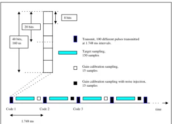
1472 T. Turunen et al.: High resolution general purpose D-layer experiment 40 bits, 160 us 20 bits 8 bits 1.748 ms

Code 1 Code 2 Code 3 Target sampling, 150 samples Gain calibration sampling, 15 samples

Gain calibration sampling with noise injection, 15 samples

Transmit, 100 different pulses transmitted at 1.748 ms intervals.

time

Fig. 1. Transmitted pulse structure and sampling arrangements.

The decoding using 40-bit FIR filtering produces data for pulse-to-pulse correlation computations, where the lag incre-ment is the same as the pulse repetition period. In the next step, the sample vector is divided into two 20-bit parts, whose parts are decoded separately and from the outputs a series of 80 µs lags is computed as an approximation of the “true power”. In this way, providing that the filters are behaving well, one avoids the need for background subtraction. Fi-nally, the 40-bit sample vector is divided into 5 pieces of 8 bits, which are decoded separately. All the possible four lag profiles at 32 µs lag increments are then computed to obtain E-layer data. Those profiles can also be used when estimat-ing the accuracy of the zero lag approximation in the D-layer by checking against the gradient of the autocorrelation func-tion near the zero lag.

The lag profile at the 80 µs delay is used here as an ap-proximation of the power. Of course the result is not true power, i.e. the zero lag of the target autocorrelation function. It is rather a lag whose weighting function in the lag domain peaks at a 80 µs delay and whose weighting function covers the delays from 0 to 160 µs. The magnitude of the lag is, in most cases, a perfectly good approximation for the power of the scattered signal and in practice, it is often enough to use the real part of the lag as an approximation, because the imaginary part is always very small compared with the real part. The estimate has a non-zero imaginary part containing line-of-sight velocity information.

In the described method, all the unwanted responses, in-cluding remote pulse cancellation, form nearly zero mean processes if the codes are properly selected. In the EISCAT radars, one must use codes which are selected beforehand, and the code sequence is then transmitted repeatedly. A ran-dom code generator can generate those codes. However, most of the randomly generated individual codes are quite poor in terms of our criteria. Computing a large number of codes and selecting those that have good properties from the application point of view leads to a much better solution. In this work, less than one code out of 1 · 106candidate codes

0 10 20 30 40 50 60 −0.2 0 0.2 0.4 0.6 0.8 1 1.2

Spatial response of E−layer part of the experiment

Position of spatial ambiguity. Main peak at position 32.

Spatial response normalized to main peak at lag 1.

Fig. 2. Spatial response of the E-layer part of the experiment

con-taining lag profiles at 32, 64, 96 and 128 µs.

passed all the tests.

It is not necessary to use boxcar weighted FIR filter coeffi-cients in the decoding. By introducing a little tapering (fourth root of cosine is used in this work), one does not lose a lot of statistics, but it is easier to find suitable codes. In particular, it is possible to find codes with exceptionally small side lobes while simultaneously forcing the side lobes to have almost an exactly zero mean distribution. In the designed experiment, a similar window is used in every decoding (the whole 40-bit decoding, 20-bit decoding and 8-bit decoding). The window is only used for convenience, but it also gives certain bene-fits. Among other things it shapes the lag domain ambiguity functions to be slightly more peaked than a triangle.

The codes used in this experiment were selected in two phases. First, a few thousand codes were selected from a set of about 150 · 106_{codes on the basis of their maximum side}

lobe amplitudes and the sum of the side lobes, simultane-ously both for 40-baud and 20-baud compressions. The divi-sion to 8 bauds was not tested for side lobe performance. The codes were further studied by running them through all the processes, which have a tendency to create a non-zero bias. This is the zero lag approximation at 80 µs delay, as well as lags 1 and 2 computed from 8-bit division. Finally, 100 codes were selected from the remaining set in such a way that they produced close to zero mean distributions simultaneously in all unwanted responses. In this coding technique, one cannot totally remove all spatial ambiguities, but a totally acceptable level can be reached even with this low number of different codes. All transmitted pulses use totally independent codes, and this gives the remote pulse rejection. One could improve this a little by checking the transmitted order of the codes in a way that the clutter from the nearest disturbing pulse be-comes minimized, but this was not done and evidently not needed.

in the pulse-to-pulse correlation part of the experiment and in the programmed experiment, the computation was finally limited to 29 lags. At the lowest altitudes of the measured ranges, especially in the EISCAT VHF radar, and in the case of the Polar Mesospheric Summer Echos, one needs longer delays. For this purpose, a special “long coherence time mode” has been included in the experiment. Data from four pulses are added together in the amplitude domain to form 25 new data vectors from the original 100 vectors and pulse-to-pulse type correlation function estimates are then computed. The lag increment now becomes about 7 ms, and 24 lags are computed in this mode. One should remember, however, that the lag domain ambiguity function contains altogether seven separate peaks.

Gain calibration, which is the only calibration needed, can be done using raw data, and one does not need to apply any decoding. Calibration data related to every other transmitted pulse contains a noise injection burst. After subtraction, one obtains the noise injection value, which is used to calibrate the gain. Both vectors contain a target signal, but it does not matter because the signal power is the same in both cases, although those two vectors do not have a single similar code in the transmission. In the designed experiment the real-time computations also include normalizations between different data types.

4 Parameters and responses of the designed experiment

It is practical to use a 4 µs baud length with the selected 40-baud code length, resulting in a 600 m spatial resolution. The experiment uses a fixed set of 100 selected codes. The codes are given in Table 1, Appendix A as hexadecimal numbers. It is straightforward to derive the required 800 different FIR filters from the codes.

Sampling starts at the 60.0 km altitude. Altogether, 150 target data samples are taken, giving 66.6 km range cover-age. This is followed by 15 samples for gain calibration. In every second radar cycle, these also contain noise injection. The total data vector after every transmitted pulse is thus 165 samples long. A 1.748 millisecond pulse repetition period is used, which gives a little over 9% rf-duty cycle. Experimen-tal arrangements are illustrated schematically in Fig. 1. One can find a more detailed formulation in Appendix A for some parts of the description given below.

The data from the complete set of 100 pulses is decoded using 8, 20 and 40 baud FIR filters compression. A window formed by using the fourth root of cosine function tapers the FIR filter coefficients used in the decoding. This window was used when searching for the codes, and it should be used for optimum performance with the given code set, although it is not absolutely necessary. Calibration power is computed without applying decoding. Finally, the lag profiles are com-puted and essentially three lag profile matrixes are formed.

In the computations, the data is normalised for obtaining convenient and safe values, e.g. from a dynamic range point of view. From the interpulse data one can compute lag

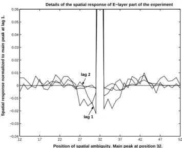
pro-12 17 22 27 32 37 42 47 52 −0.04 −0.03 −0.02 −0.01 0 0.01 0.02 0.03 0.04 0.05 0.06

Details of the spatial response of E−layer part of the experiment

Position of spatial ambiguity. Main peak at position 32.

Spatial response normalized to main peak at lag 1.

lag 1 lag 2

Fig. 3. Details of the spatial response of the E-layer part of the

experiment.

files at 32, 64, 96 and 128 µs delays, using the output from the 8-bit decoding. These four lag profiles can be used as a simple E-layer data set, giving at least the Doppler shift and electron density with certain assumptions. The spatial reso-lution of 600 m also allows for, among other things, sporadic E-layer research. Although they do not form a good estimate for the autocorrelation function, these four lag profiles are much more informative than a mere power profile. They can also be used at D-layer altitudes. The spatial response of the code is shown in Figs. 2 and 3. The normalization is done so that the main lobe at lag 1 is set to 1.

There is a tendency toward negative side lobes in lag 1 (32 µs delay) and to a smaller extent also in lag 2 (64 µs de-lay). This tendency is strongest near the main lobe and it is an unwanted effect. From practical experience it seems to be very difficult to suppress the shown behavior of spatial side lobes in lag profiles calculated from data using 8-bit com-pression when one must simultaneously keep the side lobe levels of 40- and 20-bit compressions low, and one has to keep the corresponding tendencies at the 80 µs lag profile computed from 20-bit compression at an acceptable level. A code selection was accepted when the worst case side lobes in the lag profiles computed from 8-bit compression were be-low 2% of the main lobe and the sum of the side lobes at any lag was below the 5% level. Only a few near 2% side lobes exist with the large majority of side lobes falling well below the 1% level. On the other hand, the number of side lobes in this type of coding structure is very high, and if the side lobes do not have a close to zero mean, than the cumulative side lobe error can become severe. The sums of side lobes relative to the main peak for the given code set is from lag 1 to lag 4 as follows: −1.2%, −2.5%, +2.0% and −4.9%. For comparison the cumulative side lobe error is at least +7.1% in any experiment using a 13-bit Barker code as the lowest level modulation element.

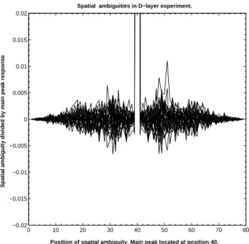
1474 T. Turunen et al.: High resolution general purpose D-layer experiment 0 10 20 30 40 50 60 70 80 −0.02 −0.015 −0.01 −0.005 0 0.005 0.01 0.015 0.02

Spatial ambiguities in D−layer experiment.

Position of spatial ambiquity. Main peak located at position 40.

Spatial ambiguity divided by main peak response

Fig. 4. Details of the spatial response of the D-layer part of the

experiment. All the lags are superposed into the same picture. The main peak is normalized to one at every lag.

The side lobe structures of the 80 µs lag and the pulse-to-pulse lags are shown superposed in detail in Fig. 4. At all lags the main lobes are normalized to unity. The envelope of the side lobes gives an indication of the worst case features. Only one side lobe, belonging to the 80 µs lag is near the 1% level. A majority of the side lobes are below the 0.5% level. Altogether, the number of side lobes in pulse-to-pulse computations is 79 and 39 in the 80 µs lag.

It is not easy to keep the sums of side lobes at a low enough level. The sums of side lobes relative to the main lobe are seen in Fig. 5. This error marginally exceeds the 4% level only in a single case, and in the majority of the cases, the error is below the 2% level. The side lobe sums are also behaving well in the sense that there are no clear systematic features. Since the side lobe structure is constant for any given set of codes, the side lobe correction can be done in the post processing of the data if the application demands it. Normally, it should not be necessary.

The lag profiles computed from coherently integrated data must be used only with a good understanding of the lag do-main ambiguity function in such a method. In particular, users are warned about the first few lags, because there the target autocorrelation function can change a lot within the lag domain ambiguity function, which contains seven separate peaks. The data is useful mainly if the target has a very long coherence time such as at lowest altitudes, perhaps during the presence of negative ions and in connection with PMSE. The performance of the codes used, shown in Table 1, was tested against 1000 totally random sets of codes using com-putations of 33 lags. The test parameters were as follows: The value of the worst side lobe, the sum of the absolute

val-0 5 10 15 20 25 30 −4 −3 −2 −1 0 1 2 3 4 5

Lags, zero lag approximation at position 1

In percents

Fig. 5. Sums of the spatial ambiguities as a function of the lag in

the D-layer part of the experiment, given in percents relative to the main peak.

ues of all side lobes and the number of side lobes exceeding the given thresholds. All computed lags were used in the comparison. The codes in Table 1 are better than any of the randomly selected codes used in all but one respect. It is easy to find a set of codes were the worst case side lobe is better than in the code set in Table 1. In fact, the mean value of the worst case side lobe in the randomly selected codes is about 2% lower than in the codes used, and the reason is that one of the side lobes (in the zero lag approximation) is much higher than the others, as seen in Fig. 4. On the other hand, as a mean, the number of side lobes with an absolute value greater than 0.3% of the main peak is almost twice as high in randomly selected codes, and if the threshold is increased to 0.4%, more than three times as many side lobes exceed the threshold in the randomly selected codes. The sum of the ab-solute values of all the side lobes is as a mean 17% worse in randomly selected codes, and none of the test code sets was found to be better in this respect than the codes used in this work.

The coding could be improved by searching for a better set of codes, which is always possible but somewhat time consuming. One could also increase the number of codes from 100 up to the point allowed by the radar hardware.

The 600 m resolution code has been designed to be a general-purpose code and uses the radar resources well. There is also a simplified 150 m resolution version available, which can be used in special applications that demand very high spatial resolution.

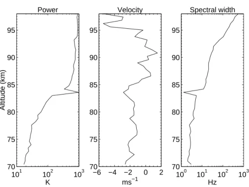
Data from some of the first tests are shown in Fig. 6 for the D-layer target, from 70 km to about 100 km altitude. The basic parameters that one obtains from the D-layer are the power, spectral width and Doppler shift of the scattered sig-nal. The curves are based on a least-squares fitting to all the available data, assuming a Lorentzian spectrum. Power is

101 102 103 70 75 80 85 90 95 K Altitude (km) Power −6 −4 −2 0 2 70 75 80 85 90 95 ms−1 Velocity

EISCAT VHF 2001−06−21 0602:30−0605:00

Fig. 6. Example data measured in Tromsø by EISCAT VHF radar at 224 MHz. Antenna pointing is vertical. The received power is expressed

as a noise temperature in Kelvin, Doppler velocity in ms−1and spectral width in Hz. Positive velocity means velocity is upwards. All three

modes of lag profiles are used everywhere in the fitting and a Lorentzian shape of spectrum is assumed, which means that E-layer altitudes are not included in the analysis. Integration time is two and one-half minutes. Polar Mesospheric Summer Echo at 83.6 km altitude is seen in all measured parameters.

shown without range correction. Integration time is two and one-half minutes, and data containing satellite echo contam-ination have been rejected.

The target power varies by almost two orders of magni-tude over the covered altimagni-tude range, and the spectral width changes by a factor of about 500. The total Doppler velocity is less than 8 ms−1 over the altitude range. Positive veloc-ity is upwards. A weak Polar Mesospheric Summer Echo is seen in the power data at 83.6 km altitude in one 600 m vol-ume. It is also seen as a local deep spectral width minimum. The spectral width of the surrounding D-layer is significantly lower below the PMSE than above it. The altitude gradient of the Doppler velocity changes signs exactly at the PMSE altitude. In general the designed experiment seems to work well.

5 Summary

A new way to measure the low altitude ionosphere by in-coherent scatter radar is described. Using a selected set of random 40-bit binary phase codes, the experiment produces D-layer pulse-to-pulse correlation lags and an approximation of power simultaneously, using a lag near the zero lag with high ambiguous range rejection. Lags are also computed for layers with a very long coherence time. Finally, a simple in-terpulse four-lag estimate is generated. In particular, this is

intended for extending the measurement to the lower parts of the E-layer, but it covers all the measured ranges. A common modulation is used in all these modes.

Acknowledgement. EISCAT is an international association

sup-ported by Finland (SA), France (CNRS), the Federal republic of Germany (MPG), Japan (NIPR), Norway (NFR), Sweden (NFR), and the United Kingdom (PPARC).

Topical Editor M. Lester thanks C. Heinselman and another ref-eree for their help in evaluating this paper.

Appendix A The computations needed in the described

D-layer experiment

The experiment is schematically shown in Fig. 1. We de-note the ith modulation bit of the mth transmitted pulse by

bmi. Any bmi can have a value +1 or −1, indicating phase

modulation by 0 or 180 degrees correspondingly. Transmis-sion occurs in the order i = 1, 2, . . . , 40. The experiment uses 100 different pulses with 40 bits modulation. After ev-ery transmitted pulse, the scattered signal from the target is sampled using a baud-matched sampling interval, i.e. iden-tical with the bit length used in the modulation. We denote the complex samples taken after transmitting the mth pulse by xmj, where j = 1, . . . , 150.

1476 T. Turunen et al.: High resolution general purpose D-layer experiment

Table A1. Codes used in the designed experiment shown as hexadecimal numbers. Conversion to binary, including the possible leading zeros

and replacing zeros with −1, gives the 100 codes of 40 bits used. Codes are transmitted with the leftmost bit first. Every entry represents one 40-baud code. The first five codes are those forming the first row in the table

A9471188B6 DB9FC23E25 899EA7F359 4D62F2EBE6 5786483299

560674268E FF1D8DD231 DBF4393AE4 FC74493AEF 37D70ACFE1

D4D16084D9 7914CD97FC CE06A416B1 CB23B4F1FC C8A403ED15

3177EF26C6 539A222785 19E2D16443 0DAE5BCFAC 32D7F49771

0B39FCC57F E53B1B59F1 A1FCDC5B8E 8225EA5307 443448ADF2

054E181BBA 26ABDDF28E 97D9BB10FA B31AA9F72E 814C72E50D

8B79933F56 0756301B8D F4BBB2E519 DEF0A959F4 B1FCB8F266

C194D38915 4C217E0959 EC7AB8F929 F75E6D2546 436AB3BBDA

B4E0A46159 C20DDC1235 44E6F3EB3A FCA937C5B4 329FDA9C9E

F20D4E120D 9437DE2B7C 36571ACFE9 4560E47A43 981A2AB623

5E985840D6 EA47CBD9C3 F7AE47CC2C A62DFAF660 ADB1CA75F2

68BBBC96E6 854C047DC5 70AC9046BA BBC27E16EA 3E4A60391A

706BADDF1A F7392EB92C 2E7240A6B2 8BDF34E65C 14C85CEC25

6A0A62A33C B96FC519B6 BB7AC8B3CA A3781C096C D0533A8171

CE990A7103 32A01A61DF 7282032BE7 9523841AF2 74E50113C5

6E104B7845 1D5BECA7D2 458D02F525 30A83AB4B1 7BA265C6FC

A99E31FBA6 30B95A5305 CBC237F569 F3A351EDE1 613ADA104D

585E6FE93A D389D8C085 4226E4B88B B5C113C445 49C4243E71

2B21C451F8 5BD386CE7C 2967C7B9F2 C597EDD0E6 E7D4D83D72

C60645EC45 A0B7351035 9503110FCF EC0C29A0E5 6F0EB85FB1

For decoding the amplitude domain data, 8 different FIR filters are needed. For decoding the total pulse, the filter coef-ficients ctmj are the modulation bits of the pulse m in reverse

order

ctmk=bm(40+1−j ), j =1, 2, ...40 . (A1)

The decoded data vector zmt for pulse m is now

zmt = 40 X j =1

xm(l−1+j )∗ctmj∗Wj, (A2)

where Wj is a weighting function. If the weighting function

used Wj =1 for every j , then (2) represents the well-known

matched filtering of phase coded data used extensively in radars, e.g. in connection with Barker codes or complemen-tary codes. Our Wj is chosen as a fourth root of cosine and

this causes a small tapering of the filter coefficients:

Wj = 4

p

cos(π(j/ k − (1 + 1/k)/2)), k = 40 . (A3) The sample zmt contains the main target contribution from

a single volume Vt. The spatial resolution along the radar

antenna beam is given by the bit length in the modulation. In addition, the sample contains smaller contributions from many other volumes. If Wj = 1 for every j , then the

spa-tial response would be given by the autocorrelation function of the code used. The Wj used modifies this a little. The

wanted volume is obtained at zero lag of this autocorrelation function, and the other lags represent the unwanted contribu-tions, namely the spatial ambiguities.

The modulations used are random. As a consequence, all the spatial ambiguities form a random zero mean process,

and the spatial ambiguities of different codes do not corre-late.

The target autocorrelation function estimate can now be computed for lags greater or equal to 1. These are the pulse-to-pulse correlation lags. For volume t at lag l, the estimate computed from one set of M codes is

acft l = M−l X m=1

zmt∗z∗(m+l)t,

M =100 in the present solution. (A4) This is done for every volume and all wanted lags and fur-ther time are averaged by repeating the process and accu-mulating like results. The lag increment is equal to the inter-pulse period. All contributions from unwanted volumes form a zero mean random process.

The next step is to estimate the power of the scattered sig-nal for every volume, i.e. the zero lag of the target auto-correlation function. Simply squaring the samples given by Eq. (A2) does not work, because one cannot separate the con-tribution of white noise, power arising from spatial ambigui-ties and power arising from a few earlier transmitted pulses, which, in spite of having different modulations, increase the noise level. This problem is circumvented by approximating the power by the value of the autocorrelation function close to the zero lag instead of exactly at zero lag, because then one can make use of the good properties of the phase coding used. This method in a different arrangement has also been used earlier in EISCAT radars (Turunen, 1986). One of the possible ways is to treat the transmitted 40-baud pulse as a two-pulse, 2 × 20 baud code and compute the lag, which is allowed by this code.

The following two filters having 20 coefficients are now formed for the transmitted pulse m.

cAmp=bm(40+1−j ), j =1, 2, . . . , 20 , (A5)

cBmq=bm(20+1−j ), j =1, 2, . . . , 20 . (A6)

Coefficients cAmpdecode the target signal created by the

first half of the transmitted pulse and the coefficients cBmq

decode the contribution of the second half of the transmitted pulse. Two decoded data vectors are now formed for every pulse m xmt = 20 X j =1 xm(t −1+j )∗cAmp∗Wj, t =1, 2 . . . , (A7) ymt = 20 X j =1 xm(t +20−1+j )∗cBmq∗Wj. (A8)

The weighting function Wj is given by formula (3), setting k =20. The filtered samples xmtand ymtrepresent the same

volume t . The wanted zero lag approximation for volume t is now acft0= M X m=1 xmt∗ymt∗ ,

M =100 in the present solution. (A9) This process is then time averaged for obtaining the required accuracy.

A simple “E-layer estimate” is also formed, which can be used to extend the range coverage above the altitude, where pulse-to-pulse correlation stops working. The com-putations are, in principle, identical to the previous zero lag approximation, where the transmitted pulse was treated as a two-pulse code, but now the pulse is treated as a five-pulse, 5 × 8 bauds code without any gaps between the pulses. Here the ambiguities disappear, because the basic code has been selected such that every subpulse has a different code. When decoded in the amplitude domain, and if the codes are truly random, the unwanted spatial responses form a zero mean

random process. Altogether, 4 lags can be computed. The details of the formulation are not repeated here.

Finally, the experiment contains a special mode for tar-gets with very long coherence time, e.g. PMSE. Coherently adding data of the type shown in Eq. (2) from 4 transmitted pulses produces 25 new data vectors, where the value ZMt

for a volume t is given

ZMt =

m=4 X m=1

z(4(M−1)+m)t, M =1, 2, . . . , 25 . (A10)

Finally, the pulse-to-pulse correlation type autocorrelation function estimate ACFLt is computed for lag L and volume t ACFLt = 25−L X M=1 ZMt ∗Z(M+L)t∗ , L =1, 2, . . . , 24 . (A11)

The response of ZMt in time domain contains four

nar-row peaks separated by an interpulse period. As a conse-quence, the resulting lag domain ambiguity function for the estimates ACFLt has seven peaks separated by one

inter-pulse period and the relative weights are 1, 2, 3, 4, 3, 2 and 1. The strongest peak is centered at a nominal delay, which is a multiple of 4L interpulse periods. One has to keep this somewhat poorly behaving time domain ambiguity function in mind when using the data.

References

La Hoz, C., M. Rietveld, G. Wannberg, and S.J Franke, The sta-tus and planned development of EISCAT in mesosphere and D-region experiments, Handbook for MAP., 28, 476–488, 1989. Lehtinen, M. S. and H¨aggstr¨om, I.: A new modulation principle for

incoherent scatter measurements, Radio Sci., 22, 625–634, 1987. Turunen, E.: Incoherent scatter radar contribution to high latitude

D-region aeronmy, J. Atmos. Terr. Phys., 58, 707–752, 1996. Turunen, T.: GEN-SYSTEM – a new experimental philosophy, J.

Atmos. Terr. Phys., 48, 777–785, 1986.

Zhou, Qihou H.: Incoherent scatter radar measurement of vertical winds in the mesosphere, Geophys. Res. Lett., 27, 1803–1806, 2000.