Distribution, growth, and transport of larval fishes and implications for population dynamics

(1)

(2)

(3)

Distribution, growth, and transport of larval fishes and

implications for population dynamics

by

Christina M. Hernández

Submitted to the Department of Earth, Atmospheric, and Planetary Sciences on October 29, 2020, in partial fulfillment of the

requirements for the degree of Doctor of Philosophy

Abstract

ABSTRACT

The early life stages of marine fishes play a critical role in population dynam-ics, largely due to their high abundance, high mortality, and ease of transport in ocean currents. This dissertation demonstrates the value of combining larval data, collected in the field and the laboratory, with model simulations. In Chapter 2, anal-yses of field observations of ontogenetic vertical distributions of coral reef fish re-vealed a diversity of behaviors both between and within families. In Caribbean-wide particle-tracking simulations of representative behaviors, surface-dwelling larvae were generally transported longer distances with greater population connectivity amongst habitat patches, while the evenly-distributed vertical behavior and downward onto-genetic vertical migration were similar to one another and led to greater retention near natal sites. However, hydrodynamics and habitat availability created some lo-cal patterns that contradicted the overall expectation. Chapter 3 presents evidence of tuna spawning inside a large no-take marine protected area, the Phoenix Islands Protected Area (PIPA). Despite variation in temperature and chlorophyll, the larval tuna distributions were similar amongst years, with skipjack (Katsuwonus pelamis) and Thunnus spp. tunas observed in all three years. Backtracking simulations indi-cated that spawning occurred inside PIPA in all 3 study years, demonstrating that PIPA is protecting viable tuna spawning habitat. In Chapter 4, several lines of lar-val evidence support the classification of the Slope Sea as a major spawning ground for Atlantic bluefin tuna with conditions suitable for larval growth. The abundance

(4)

of bluefin tuna larvae observed in the Slope Sea aligns with typical observations on the other two spawning grounds. Age and growth analyses of bluefin tuna larvae collected in the Slope Sea and the Gulf of Mexico in 2016 did not show a growth rate diﬀerence between regions, but did suggest that Slope Sea larvae are larger at the onset of exogenous feeding. Collected larvae were backtracked to locations north of Cape Hatteras and forward tracked to show that they would have been retained within the Slope Sea until the onset of swimming. As a whole, this thesis presents valuable contributions to the study of larval fishes and the attendant implications for marine resource management.

Thesis Supervisor: Joel Llopiz Title: Associate Scientist

(5)

Acknowledgments

The work presented in this dissertation was supported by funding from the National Science Foundation Graduate Research Fellowship Program (to C.M.H.), the Woods Hole Oceanographic Institution Ocean Life Institute (Grant 22569.01 to J. Llopiz and C.M.H.), the Adelaide and Charles Link Foundation, the Phoenix Islands Pro-tected Area Trust, the J. Seward Johnson Endowment in support of the Woods Hole Oceanographic Institution’s Marine Policy Center, and the WHOI Academic Programs Oﬃce.

There are so many people that have made this thesis possible, both materially and by shaping me into the person I am and the scientist I’m still becoming.

Thank you to my advisor, Joel Llopiz, for taking a chance on me as a summer student (in 2013!) and for your steadfast support of me ever since. Thank you to Michael Neubert, my “second advisor,” for nurturing my mathematical side and helping me dream scientific dreams. Thank you to David Richardson for opening doors for me to work on bluefin tuna larvae and for being one of my most trusted co-authors. Thank you to Stephanie Dutkiewicz for providing encouragement and *ahem* reasonable limits to what one person should try to accomplish in their thesis. Thank you to the WHOI Academic Programs Oﬃce, the Joint Committee for Biological Oceanography, the WHOI Biology Department, and MIT-EAPS for pro-viding me with so many opportunities for learning and growing.

Many co-authors and labmates made this work possible– and far more enjoyable. Sarah Glancy, Justin Suca, Martha Hauﬀ, Helena McMonagle, Paul Caiger, Julia Cox, and Andy Jones all made being part of the Llopiz (FOLFE) lab so much better. Thank you to Kristin Gribble, Hal Caswell, Silke van Daalen, Julie Kellner, Irina Rypina, Randi Rotjan, Kathy Mills, Andy Pershing, Jan Witting, Ke Chen, Ciara Willis, Simon Thorrold, Katey Marancik, Claire Paris, Ana Vaz, Robert Cowen, Su Sponaugle, Katie Shulzitski, and Ben Jones for working on various projects with me, much of which forms this thesis. Thank you to the crew and science parties of numerous cruises for making this work possible including: S261, S268, S274, HB1603, GU1608, HB1704, and GU1702.

I also owe a debt of gratitude for my growth as a scientist (and a person) to my friends, the SWMS community, and my co-conspirators in the fight for greater justice, equity, diversity, and inclusion in science: Lizzie Wallace, Rachel Housego, Ryan O’Shea, Kassandra Costa, Alex Pan, Mira Armstrong, EeShan Bhatt, Gabi Serrato Marks, Mara Freilich, Suzi Clark, Jen Karolewski, Joleen Heiderich, Alexa Sterling, Anna Robuck, Sophie Chu, Kwanza Johnson, Jessica Dabrowski, Billy Shinevar, Casey Zakroﬀ, Julia Middleton, Paris Smalls, Adam Subhas, Henri Drake, Ashley

(6)

Bulseco, and probably 50 more people I’m failing to mention. Oh, and shout out to Arnault Le Bris for winning our bet.

Thank you to EAPS Cookie Hour and Jeﬀrey Mei for introducing me to Harry Matchette-Downes. I’m so happy that you’re by my side, Harry. I can’t wait for our next adventure.

Finally, I’d like to list a few people who were instrumental in shaping me into someone who would even end up in the Joint Program. My parents, Cathy Chambers and Albert Hernández, my brother, Steven Hernández, and my grandmothers, Judy Chambers and Doris Pérez, have always believed I was capable of anything I set my mind to. I was also blessed to have some amazing mentors and cheerleaders in high school and college: June Van Thoen, David Sabella, Robert Sabella, Samuel Baskinger, Joe Kyle, and Jerry McManus. Thank you for seeing me.

(7)

Chapter 1 General Introduction

As human populations grow and anthropogenic influence stretches to every inch of the globe, there are few resources that are not directly impacted by humans. Marine resources, specifically fish and shellfish protein, represent one of the only large-scale ‘wild harvest’ industries. Some species are affected by human activities without being directly targeted, either through bycatch in commercial fisheries or through ecosystem effects such as eutrophication, dredging, and habitat degradation. As valu-able fisheries species experience anthropogenic influences, resource managers work to understand and predict the productivity of these stocks, either to set quotas for sus-tainable fisheries or to protect species and ecosystem health. Studies of spawning behavior and early life history stages offer valuable contributions towards the goal of improved management.

The importance of the early life stages of fishes has been recognized since the early 1900s. The seminal work by Johan Hjort (1914) used cohort analyses and novel aging techniques to demonstrate that strong year-classes could dominate a given fishery for several years. Hjort attributed much of the variation in year-class strength to

(11)

eﬀects during a “critical period,” which he identified as the first-feeding period of recently hatched larvae. Following on from Hjort’s work, important contributions to fisheries oceanography and early life history theory include the match-mismatch hy-pothesis which generalizes Hjort’s “critical period” hyhy-pothesis to focus on the relative phenology of larvae and their planktonic food sources throughout the larval period (Cushing, 1990), the member-vagrant hypothesis wherein transport and retention processes play a crucial role in both stock delineation and stock dynamics (Iles and Sinclair, 1982), and the stage-duration or “bigger is better” hypotheses wherein faster growth and/or development decrease cumulative mortality due to predation (Cush-ing, 1990; Miller et al., 1988). Edward Houde also made important contributions to our understanding of the relationships among temperature, growth rate, and mor-tality of larval fishes, and latitudinal patterns in these factors (Houde, 1989; Houde, 1997).

Much of the work mentioned thus far focused on mid- to high-latitude fisheries species, such as Atlantic herring, Atlantic cod, and other species in the family Ga-didae (Hjort, 1914; Houde, 1989; Iles and Sinclair, 1982). A hallmark of these temperate environments is the strong seasonality of plankton production, which in-fluences the phenology of both spawning and larval development. A theory like the match-mismatch hypothesis is less relevant in the tropics, where seasonal variation in plankton biomass is much weaker (i.e., larval food availability is more constant). The other important characteristic of Atlantic herring that influenced these foun-dational theories is that they are a pelagic species– their ideal habitat tracks water masses and oceanographic features rather than bottom type or structure.

On the other hand, many species of fish settle onto bottom habitat after their pelagic larval period, to live as demersal adults with varying levels of site fidelity. Bottom habitat with the correct features or substrate is often available in a patchy

(12)

distribution. As the distance between high-quality habitat (or the risk of predation along that distance) increases, adult fish are more likely to show high site fidelity. However, pelagic larvae can be transported amongst these patches, linking the var-ious habitat patches into a metapopulation (Hanski, 1998). A critical question for the study and management of coral reef fish populations was the degree to which individual populations were open or closed (Cowen et al., 2000; Cowen et al., 2006). If a population is completely closed, then its population dynamics are set by the production of oﬀspring by adults within that same patch of habitat. In a completely open or fully connected population, the population dynamics in any one habitat patch depend on the supply of larvae from all of the other patches.

The reality, for most populations, is somewhere in the middle of the open-closed spectrum, and depends on a plethora of both biotic and abiotic factors (Cowen and Sponaugle, 2009). The local and regional hydrodynamics, as well as the distribution of habitat patches clearly play a role in the connectivity of a metapopulation. The pelagic larval duration– the amount of time that larvae spend developing before seek-ing settlement habitat– sets an upper limit on larval dispersal distance (Sponaugle et al., 2002). Individual-based biological-physical models have allowed us to move beyond the early concept of larvae as passive particles to understand the importance of larval traits, such as vertical distribution behaviors (Paris et al., 2013; Vaz et al., 2016) and swimming abilities (Rypina et al., 2014). Despite the increased availabil-ity of sophisticated models that can incorporate larval behavior, the vast majoravailabil-ity of recent modeling studies of larval dispersal continue to treat larvae as passive tracers (Swearer et al., 2019). Furthermore, those studies that do incorporate larval behav-ior tend to focus on a single species, or comparisons between very diﬀerent species (Faillettaz et al., 2018; Kough and Paris, 2015; Petrik et al., 2016). Therefore, the general consequences of small changes in larval behavior between otherwise quite

(13)

similar species is not well understood.

Connectivity and its impact on the population dynamics at any given reef site are important considerations in the management of both harvested and protected reef populations. Studies of connectivity, through genetic, chemical tagging, and com-puter simulation approaches, have influenced marine protected area management (MPA) by highlighting the importance of MPA size and the potential value of MPA networks (Botsford et al., 2001; Ross et al., 2017; Watson et al., 2011). A general-ized, trait-based approach could help to fill our knowledge gap with respect to the role of larval behaviors, while also providing managers with a method to estimate connectivity when they are unable to undertake a new study targeting their location or species of interest.

Regardless of the causal mechanisms, the fact remains that tiny proportional changes in the survival or growth of oﬀspring, or in the number of settlers arriving at a given patch of habitat, can have outsized impacts on cohort strength and, by extension, population dynamics. This fact arises from the prodigious fecundity of fishes (thousands to millions of eggs per individual) and the high mortality rates dur-ing early life stages (>99%). However, eggs and larvae disperse quickly in the ocean and therefore are often present at low density or in a patchy distribution that makes systematic sampling diﬃcult and costly. Furthermore, larvae may sample a range of conditions during their pelagic period of days to months, complicating our ability to identify the relevant covariates to estimates of growth and mortality. Therefore, despite our long-term understanding that early life history conditions modulate pop-ulation dynamics of fishes, these stages are still generally poorly-represented in stock assessment models and management frameworks.

In spite of these diﬃculties, studies of the early life history conditions of harvested or protected species continue to have important benefits for fisheries science and

(14)

management. In Atlantic bluefin tuna, the discovery of larvae in the Slope Sea has re-opened important questions about age-at-maturity, stock mixing, and stock productivity (Richardson et al., 2016 and this thesis, Chapter 4). Larval distributions can be combined with age analysis and particle tracking simulations to provide insight into probable spawning locations (by running the simulations backwards) and larval transport to settlement locations (by running the simulations forwards). Particle tracking simulations are employed in all three projects presented in this thesis. In Chapter 2, I used forward-tracking simulations to test hypotheses about how larval vertical behaviors impact larval dispersal and population connectivity for coral reef fishes. In Chapters 3 and 4, I used backward-tracking simulations to estimate the likely spawning sites for highly-migratory species in locations where we have analyzed larval distribution, age, and growth, but where we have very limited data on adult spawning behavior. In Chapter 4, I also use forward-tracking simulations to explore the transport and retention conditions in a highly dynamic ecosystem.

Because of the high number of fish eggs released and the extremely high mortality rates that the larvae face during their first weeks of life, the removal of larvae from the environment has a relatively small impact on the population. Compared to the millions of larvae that might be present across an ecosystem, the few hundred of any given species that we might remove for larval studies will not have an appreciable eﬀect on the mortality rate– and many of the larvae we sample would have died anyway. Therefore, sampling of eggs and larvae can be a lower-impact way to study fish populations, particularly in locations where fishing is prohibited. In Chapter 3, I demonstrate how larval sampling inside a large no-take Marine Protected Area (the Phoenix Islands Protected Area, PIPA) can enable us to study the spawning of highly-migratory species of tunas that are both ecologically and economically valuable. Furthermore, larval studies were more feasible in this remote protected

(15)

area than adult tagging or maturity studies because a plankton net can be deployed from a smaller vessel with less-specialized expertise and equipment. The highly repeatable nature of plankton studies has also enabled us to build a multi-year time series of tuna larvae in PIPA.

Fish otoliths are fantastic tools that unlock a wealth of information. These cal-cium carbonate structures, essentially fish ear bones, record daily variations in feed-ing and growth as differences in the density of the calcium carbonate matrix. These density differences are visible as concentric rings or growth increments. We can estimate larval age in days from the number of rings present in the otoliths, and the width of each ring is a proxy for daily growth rate. Furthermore, since lar-val size is correlated with otolith radius, we can also use otolith measurements to back-calculate the size of each fish on previous days of its life. These otolith met-rics record the overall combined effect of several intrinsic and extrinsic mechanisms that can cause variations in growth, including temperature, food availability, and genetic or species-level differences. With larval otoliths, we can compare the larval conditions for the same species spawning at different locations or times of year, and gain greater insight into the vulnerability or productivity of different stock segments. In Chapter 4, I took this approach to explore whether Atlantic bluefin tuna larvae spawned in the Slope Sea differ significantly in their growth from those spawned in the Gulf of Mexico. Because larval growth rate is thought to be related to survival, differences in larval growth rates between two stock segments imply differences in the contribution of those two groups to overall stock productivity. I also employed otolith analyses for Chapter 3, in which I built a relationship of larval length and age. Then, I ran backtracking simulations to generate a map of estimated relative spawning output that corresponded to our observed larval distributions.

(16)

tropical Pacific to the temperate Atlantic and include both highly-migratory and demersal site-attached species. They combine field, laboratory, and modeling meth-ods to draw new connections between early life history of fishes and the population dynamics of managed species and ecosystems. They highlight gaps in our knowl-edge of valuable and intensively-studied species. Through this dissertation, I seek to fill a few of those gaps and to demonstrate the value of continuing to invest in the sampling and study of larval marine fishes.

(17)

Chapter 2 Larval traits drive patterns of marine

dispersal and connectivity

2.1 Abstract

Larvae of coral reef fishes have taxon-specific traits that can influence larval trans-port, but we lack a clear understanding of how such traits, specifically vertical distri-bution behaviors, influence dispersal and population connectivity. We analyzed field observations of larval vertical distribution behaviors for 23 taxa of coral reef fish. We selected three representative behaviors—surface-dwelling, evenly-distributed, and on-togenetic vertical migration (OVM)—and two pelagic larval durations (PLDs) to pa-rameterize a biological-physical model of larval dispersal throughout the Caribbean Sea. When all releases across the Caribbean were combined to generate dispersal kernels, the shorter PLD reduced dispersal, but for a given PLD, surface-dwelling be-havior generally led to longer-distance dispersal, lower regional retention, and higher population connectivity than the evenly-distributed and OVM behaviors. However,

(18)

there was region-specific variability in these trends. The same combination of traits led to diﬀerent retention and connectivity outcomes depending on the region of larval release, demonstrating the complex interplay among larval traits, oceanic currents, and habitat availability.

2.2 Introduction

Due to the prevalence of a pelagic larval phase across marine taxa, and the ease with which propagules are dispersed in the marine environment, a fundamental aim of ma-rine ecology is to understand the processes governing the transport of pelagic larvae and their subsequent arrival at suitable settlement habitat (Cowen and Sponaugle, 2009; Pineda et al., 2007). The connectivity of suitable habitat patches has impli-cations for population persistence and community dynamics, including the resilience and replenishment of disturbed communities (Aiken and Navarrete, 2011; Hastings and Botsford, 2006; Thrush et al., 2013). Shallow-water coral reefs are a canonical example of patchy habitat, and the study of larval population connectivity is criti-cally important to conservation of the reefs and management of their associated fish populations (Botsford et al., 2001; Burgess et al., 2014).

Dispersal modeling is a valuable tool for investigating connectivity of reef fish populations (Werner et al., 2007). In the past 15 years, major advances in computing power have enabled the development of high-resolution models of ocean currents and their use in increasingly complex biological-physical models. These models can now incorporate more biologically-realistic larval behaviors, notably vertical distribution, vertical migration, and horizontal swimming ability (Brochier et al., 2008; Edwards et al., 2008; Faillettaz et al., 2018; Paris et al., 2013; Petrik et al., 2016; Rypina et al., 2014; Staaterman et al., 2012; Sundelöf and Jonsson, 2012; Vaz et al., 2016).

(19)

Regardless of the importance of larval movement and the existence of models that are able to simulate such behaviors, most recent Lagrangian models of larval dispersal have considered larvae as passive tracers (Swearer et al., 2019), highlighting the need to understand the broad consequences of larval behavior.

Across the many taxa of coral reef fish, a wide variety of larval traits, includ-ing morphology, diet, developmental rate, swimminclud-ing abilities, sensory abilities, and depth preferences have been documented. Adult reproductive traits, such as fecun-dity, as well as spawning season, periodicity, and location can also vary between and within species. Any of these traits can directly or indirectly affect larval dispersal and connectivity. For example, innate or environmentally driven differences in devel-opmental rates affect the pelagic larval duration (PLD), or the length of time in the water column, which sets an upper limit for the scope of larval dispersal (Sponaugle et al., 2002). The few studies on the depth distributions of larval coral reef fish during their pelagic phase highlight taxon-specific behaviors (Cha et al., 1994; Hue-bert et al., 2010; Irisson et al., 2010; Leis, 1991), and, due to vertical differences in ocean current velocity, it seems likely that such differences should influence dispersal (Huebert et al., 2011; Irisson et al., 2010). Of particular interest are patterns in vertical distributions related to larval age or ontogeny. Ontogenetic vertical migra-tion (OVM) is characterized by a downward trend in depth distribumigra-tion with larval age (Irisson et al., 2010; Paris and Cowen, 2004) and, amongst modeling studies that include depth behavior, OVM behavior is commonly used (Butler et al., 2011; Kough et al., 2013; Staaterman et al., 2012; Truelove et al., 2017; Vaz et al., 2016; Yannicelli et al., 2012). Additionally, OVM has been proposed as an adaptive mechanism for constraining larval dispersal with Ekman transport, particularly in locations where sub-surface flow can deliver larvae back to shore (Paris and Cowen, 2004). However, it is not clear how widespread this behavior is across taxa or how regional variability

(20)

in flow regimes and bathymetry modulate the eﬀect of this behavior on retention, so further study of its prevalence and its consequences for dispersal is warranted.

A generalized and trait-based approach to modeling pelagic larval connectivity would provide important insights into the relative influence of various larval traits, and would enable more reliable predictions of connectivity scaling based on larval traits. We report here the vertical behaviors observed from extensive field sampling for the larvae of 23 taxa of coral reef fish. Based on these field observations, we se-lected three representative larval distribution behaviors, as well as two pelagic larval durations (PLDs), to examine how these behaviors and PLDs influence dispersal and connectivity across the Caribbean region. To do this, we used the Connectivity Mod-eling System (Paris et al., 2013), which is a biological-physical Lagrangian particle tracking model that simulates observed distributions of larval traits and settlement to reef habitat, enabling the estimation of dispersal probability and potential connec-tivity. Our study provides insight into how life history traits might enable population persistence for fish living in patchy coral reef habitat.

2.3 Methods

2.3.1 Field Sampling

Between January 2003 and December 2004, a transect of 17 stations across the Straits of Florida was sampled monthly for fish larvae [details in (Llopiz and Cowen, 2008)]. Larvae were collected with a 4-m2 _{multiple opening-closing net and environmental}

sensing system (MOCNESS) (Guigand et al., 2005; Wiebe et al., 1976) and a 1 x 2 m neuston net, both with 1-mm mesh. The MOCNESS nets each sampled approximately 25 m of water depth, with four target depth bins: 0-25 m, 25-50

(21)

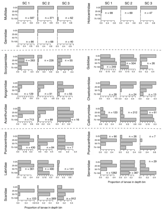
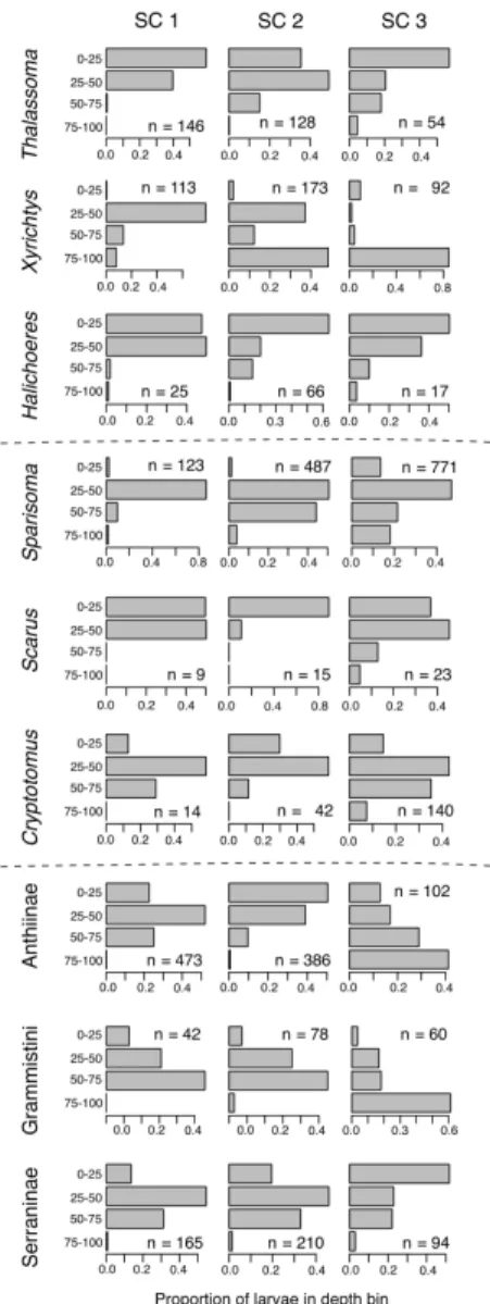
Figure 2-1: Selected ontogenetic vertical distributions. Each row of panels represents a diﬀerent taxon. The first 7 rows are Family-level taxa, and the final 2 rows are at a lower taxonomic level: Grammistini is a tribe in the Family Serranidae, and Xyrichtys is a genus of the Family Labridae. The columns of sub-panels refer to size classes (SC) 1 through 3 that represent respectively 25, 25, and 50% of the observed size range. Each sub-panel shows the proportional abundance in 4 depth bins in the upper 100m, and the total sample size (n) for each taxon and size class.

(22)

m, 50-75 m, and 75-100 m. The neuston net sampled the upper 0.5 m of the water column. Nets were outfitted with flowmeters to estimate the volume of water sampled during each tow. In the lab, larvae were identified to the family, subfamily, tribe, or genus level. Of the 55,603 coral reef fish larvae that were identified, a subset of 2530 were measured to provide the size-class-specific vertical distribution results presented here. Measured larvae came from every other monthly cruise (starting with Feb, with Jan and March also included for 2003) and every other station across the Straits of Florida (for a total of 8 stations). Within each station–depth bin combination, all larvae for each taxon were measured for standard length up to a maximum of 30 randomly selected individuals.

2.3.2 Data Analysis

In order to identify common vertical behaviors, we calculated proportions at depth, with size (as a proxy for age), for 23 coral reef fish taxa in the Straits of Florida collections: 14 families, 2 subfamilies, 1 tribe, and 6 genera. For each study taxon, measured larvae were split into three size classes, representing 25, 25, and 50% of the observed size range. There were some particularly large larvae that were outliers in the size distribution, which were 2.86-13.09 mm longer than the next longest larva of that taxon. To have a reasonable sample size in each size class, we adjusted the length range using the second-longest larva in Scorpaenidae, Acanthuridae, Chaetodontidae, Scaridae, Gobiidae, and Pomacanthidae, and the third-longest larva in Pomacentri-dae. For taxa at lower taxonomic levels, we adjusted the size range using the second-longest larva in Anthiinae and Sparisoma, and the third-second-longest larva in Serraninae. These particularly large larvae were still included in size class 3 for the purpose of calculating proportions at depth.

(23)

Larvae were also separated into depth bins. The MOCNESS net samples were classed according to their target depth range (0-25, 25-50, 50-75, and 75-100 m). Surface (neuston) net samples were combined with the 0-25 m MOCNESS depth bin. Larval abundance (ind. m-2_{) for each net was calculated as: a}

i = ni/vi ⇤ hi,

where ni is the number of individuals collected in the net, vi is the total volume

filtered by that net, and hi is the range of depth sampled (Irisson et al., 2010). The

range of depth sampled was set to 0.5 m for the neuston nets, but for the MOCNESS nets, was determined from the actual minimum and maximum depths recorded.

After classifying the larvae according to size and depth, all stations were pooled to determine the mean abundance of each size class and depth bin combination. For each taxon, we produced proportions at depth for each size class. The proportion in a given depth bin is the sum of all sample abundances in that depth bin, divided by the sum of all sample abundances across the four depth bins.

2.3.3 Model simulations

We used the Connectivity Modeling System (CMS) (Paris et al., 2013), an open-source individual-based biological-physical model, together with a 3D field of ocean currents from the Hybrid Coordinate Ocean Model (HyCOM) Global (1/12° resolu-tion) and Gulf of Mexico (1/25° resoluresolu-tion) data. While HyCOM does have vertical velocities available, we use only the horizontal velocities, at the 7 available depths in the upper 100 m.

A main focus of this study is the use of the depth assignment module of CMS. This module moves particles by a single depth bin at each time step, so that the simulated depth distribution is as similar as possible to a user-provided matrix of the proportions at depth at various ages throughout the PLD. Note that if all larvae begin

(24)

at the same depth, it may take several time steps for the population of particles to match the intended vertical distribution. This study utilizes three vertical behaviors: (1) surface-dwelling larvae, held at 1 m depth; (2) larvae that are evenly distributed across 9 depth bins in the upper 100 m; and (3) a generalized 9-depth OVM behavior based on five taxa (two families: Pomacanthidae and Pomacentridae; one subfamily and one tribe: Anthiinae and Grammistini, both in the family Serranidae; one genus: Xyrichtys in the family Labridae) (Figure 2-9). For the evenly-distributed and OVM larvae, the 9 depths we used were 4, 12.5, 21, 31.25, 43.75, 56.25, 68.75, 81.25, and 93.75 m.

We calculated a generalized OVM distribution by averaging the observed propor-tions at depth from the five taxa that demonstrated OVM and then smoothing that distribution to 9 depths (Figure 2-9). First, we took the average value across taxa of the proportion in each of the 4 observed depth bins, and re-normalized the average proportions to sum to 1. We then used the “density” function in R to estimate a ker-nel density curve from the 4-depth average proportions, and used the “integrate.xy” function in the R package “sfsmisc” to estimate the area under the kernel density curve for 9 depth bins, centered on the depths listed above.

To simulate settlement and calculate connectivity, we used the seascape mod-ule in CMS. When this modmod-ule is in use, particles that pass into one of the user-defined polygons during a specified competency period are considered settled and stop moving. We used the same 261 polygons used in a previous Caribbean-wide study (Cowen et al., 2006) based on the Coral Reef Millennium Mapping dataset (Andréfouët, 2008), with a 9 km buﬀer and a maximum width of 50 km in the along-shore direction (Figure 2-12). This buﬀer is used to incorporate a wide range of near-shore processes that are not present in models of this scale, including physical and behavioral phenomena.

(25)

Because we used shallow-water coral reefs as our target settlement habitat while focusing on particle behaviors down to 100 m, some polygons would be more ac-cessible to simulated competent larvae in the surface simulations than to simulated competent larvae in the evenly-distributed or OVM simulations. To account for this, we specified that all particles in the evenly-distributed and OVM simulations would use a shallow water distribution at locations where HyCOM data were unavailable at 100 m. The shallow water distribution moves particles to an even distribution across 3 depths in the upper 25 m (4, 12.5, and 21 m).

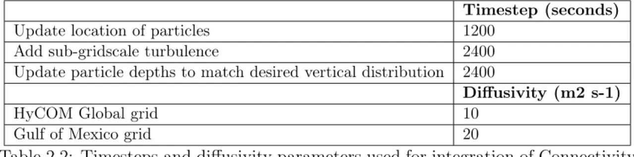
We also used the turbulence module in the CMS, which adds a random kick to particle velocities and is integral to the probabilistic framework of the model. These simulations used horizontal diﬀusivity components of 10 and 20 m2 _s-1 _{for the}

Global and Gulf of Mexico HyCOM grids, respectively (Table 2.2). We did not use a vertical diﬀusivity coeﬃcient because we used vertical behaviors in all simulations. The timesteps used for integration of the CMS model are given in Table 2.2.

Spawning was simulated by releasing 1000 particles from each polygon at mid-night of each day between January 1, 2004 through December 31, 2008. In general, release points are at the centroid of the polygon, except when this would place the particle on “land” according to the HyCOM landmask. For these release sites that cannot coincide with the polygon centroid, they were manually moved into the “ocean,” either within or close to the polygon.

We selected two durations that correspond with peaks in the distribution of reef fish PLDs reported in a synthesis paper (Mora et al., 2012). Simulated larvae were competent to settle starting on day 20 in the “short” PLD simulations, representative of taxa such as the bicolor damselfish (Stegastes partitus) (Sponaugle and Cowen, 1996), as well as several other fishes in the families Labridae and Pomacentridae (Mora et al., 2012; Victor, 1986). In contrast, for the “long” PLD simulations,

(26)

simulated larvae were competent to settle starting on day 40, representative of taxa such as the bluehead wrasse (Thalassoma bifasciatium) (Sponaugle and Cowen, 1997; Victor, 1986), as well as several other species in the families Labridae and Serranidae (Mora et al., 2012). In both cases, larvae remain competent to settle for a period of 10 days.

We do not include mortality in our model simulations, because it is insufficiently constrained and it is unlikely to change our main conclusions. Daily larval mortality rates should vary spatially (horizontally and vertically), with larval ontogeny, and across taxa, but these nuances are extremely difficult to estimate and are essentially unknown for reef fish larvae. Thus, models tend to use a constant daily mortality rate, which, if done so here, should not affect the conclusions we draw when comparing how traits influence connectivity and dispersal.

2.3.4 Analysis of simulation output

The model output was processed using MATLAB 2019a. Post-processing analyses were done only for larvae that successfully settled. We calculated larval dispersal kernels using the total dispersal distance for all successful larvae from a given simu-lation (i.e., a combination of behavior and PLD length). These distances were binned at 50 km intervals (i.e., the approximate size of each polygon) from 0 to 3000 km, and the frequency of occurrence in each bin was normalized such that the sum of all bins is 1. We also note that the dispersal distance is the total distance a particle traveled, not the straight-line distance between release and settlement locations.

We defined retention as the proportion of successful larvae from a given release site that settle in the habitat polygon corresponding to that release site. Following the geographical regions in Cowen et al. (2006), we summarized retention on a

(27)

regional basis as the mean value of retention from all polygons within a region. Connectivity matrices were created to display the probability of larval transport from a series of source nodes (the rows, i) to the receiving nodes (the columns, j). Each (i, j) entry is the proportion of settlers from source node i that settle in receiving node j; the sum of each row of the connectivity matrix is 1.

To address how behavior influenced connectivity, independent of the eﬀect of behavior on settlement probability, we defined a matrix, C, that measures the relative change in larval transport due to behavioral diﬀerences. Matrices A and B contain the counts of larvae transported from source node i to receiving node j under two behavioral scenarios. The entries of the matrix C are cij = _1/2(aaij_ijb_+bij_ij₎. This method

scales the diﬀerence by the average of the two matrices, such that the comparison matrix C is symmetrical for pairwise comparisons. However, this method cannot distinguish connections that change from 0 to 1 transported particle from those that change from 0 to 1000 transported particles. Connections that appear to be behavior-dependent, but which are formed by a single transported particle may be due more to stochasticity in the model, as opposed to demonstrating a true new connection under one of the behaviors. To focus on connections, both behavior-dependent connections and those that are maintained between behaviors, that are less aﬀected by stochastic transport events, we mask source-receiver pairs where the number of transported particles is 1000 or fewer in both A and B.

2.4 Results

Amongst the 14 families, 3 subfamilies, and 6 genera investigated for ontogenetic patterns in larval vertical distribution, our analysis revealed a wide variety of be-haviors (Figures 2-1, 2-6, and 2-7). A persistent association with surface waters was

(28)

seen in 3 families (Mullidae, Holocentridae, Figure 2-1; Gerreidae, Figure 2-6; also see Figure 2-8). A downward ontogenetic vertical migration was evident in 2 families (Pomacentridae and Pomacanthidae, Figures 2-1 and 2-6), 1 subfamily (Anthiinae, Figure 2-7), 1 tribe (Grammistini, Figure 2-1), and 1 genus (Xyrichtys sp., Figure 2-1). In the other taxa, larvae showed almost no depth preference (e.g., Gobiidae and Scorpaenidae, Figure 2-1), a relatively consistent depth preference (e.g., Apogonidae, Figure 2-1; Chaetodontidae, Figure 2-6), or widened their preferred depth range with ontogeny (e.g., Acanthuridae, Figure 2-1; Callionymidae, Figure 2-6).

To investigate the implications of these observed behaviors for larval dispersal and population connectivity, we selected three generalized larval behaviors for the dispersal simulations: (1) surface-dwelling, (2) evenly distributed across depths, and (3) ontogenetic vertical migration (hereafter, OVM). The OVM behavior is a com-posite based on taxa that exhibited this behavior (Figure 2-9). We selected two PLDs, “short” (20-30 d) and “long” (40-50 d), that are highly representative of coral reef taxa (Mora et al., 2012).

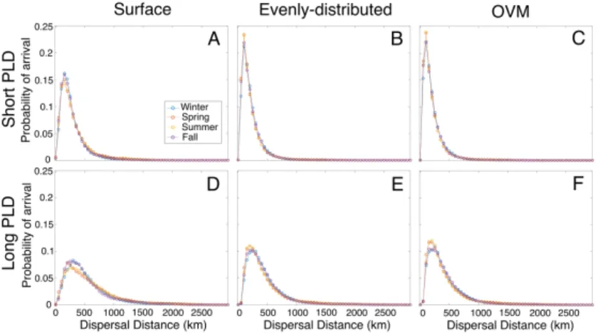
Dispersal kernels, representing the probability of larval settlement at a range of distances from release site, showed higher probability of long-distance dispersal for surface-dwelling than for the other two behaviors (Figure 2-2). The median dispersal distance of surface-dwelling larvae was greater than that for the evenly-distributed and OVM larvae, by 39-47% for the short PLD simulations, and by 29-39% for long PLD simulations. Surface-dwelling larvae also had a slightly higher probability of settling: probability of success in the short PLD simulations was 43% for surface-dwelling larvae, while evenly-distributed and OVM larvae experienced 38-39% successful settlement. In the long PLD simulations, settlement success for surface-dwelling larvae was reduced to 38% and 29-30% for evenly-distributed and OVM larvae.

(29)

Figure 2-2: Overall dispersal patterns. Dispersal kernels of successfully settled larvae for combinations of larval behavior and pelagic larval duration (PLD). The kernels are plotted as probability densities in 50-km wide bins and frequencies are normal-ized such that the sum of all bars is equal to 1. The median dispersal distance is numerically displayed and shown as a vertical dashed line. Note that all 6 sub-panels have the same horizontal and vertical axes. (Rows) Three larval behavior simula-tions were conducted: surface-dwelling, evenly-distributed, and ontogenetic vertical migration (OVM). (Columns) Short and long PLD simulations correspond to 20-30 days and 40-50 days, respectively.

Our focal traits, vertical distribution behavior and PLD, have markedly stronger eﬀects on dispersal than the eﬀects due to season or year. Dispersal kernels did not have strong seasonal variability in any of the 6 experiments (Figure 2-10). Median

(30)

dispersal distance between seasons varied by 0-14%, with the greatest diﬀerence seen between the summer and fall quarters for surface-dwelling larvae with long PLDs (Table 2.1). Likewise, dispersal kernels look very similar amongst the 5 years of simulations, with the greatest variability seen in the surface-dwelling larvae (Figure 2-11), as their transport is influenced by wind-driven circulation.

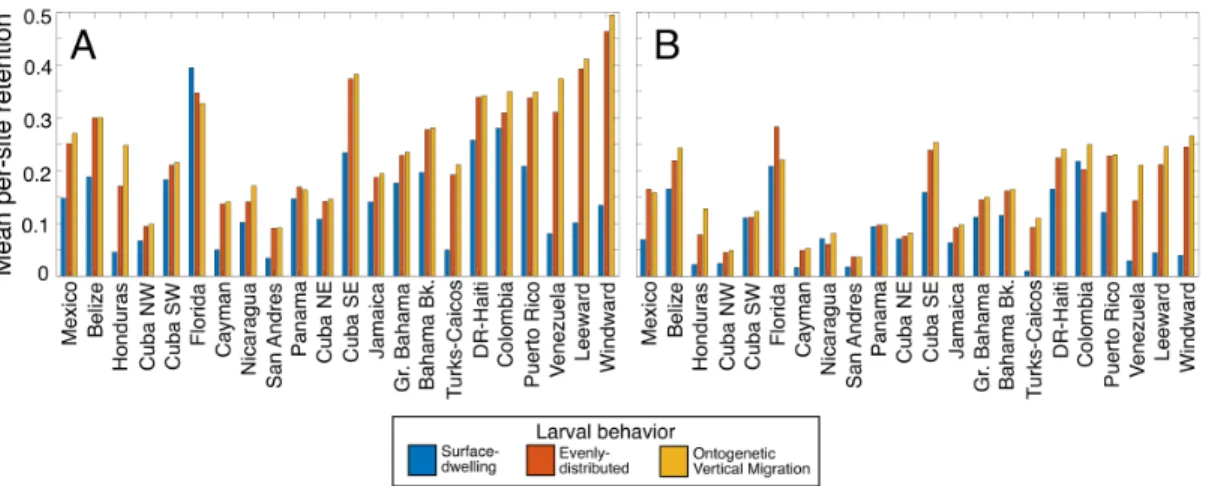
Figure 2-3: Mean regional retention, by behavior and pelagic larval duration (PLD). The height of each bar is the mean value of retention for all habitat polygons in each region, where retention is the proportion of successful larvae that settled in the same habitat polygon as their release site. Regions are arranged roughly west to east. Short PLD simulations (A) were 20-30 days long, and long PLD simulations (B) were 40-50 days long. For a map of regions, see Figure 2-12.

We examined retention by calculating the proportion of successful larvae that settled in the same habitat polygon as they were released from, and then summa-rized for each geographic region (Figure 2-12) using the mean regional retention. Overall, ontogenetically migrating and evenly-distributed larvae experienced greater retention than surface-dwelling larvae (Figure 2-3). Time spent in the plankton (PLD) decreased retention in most of the regions. However, the eﬀect of surface-dwelling behavior on retention appears strongest in the eastern Caribbean regions of

(31)

Turks and Caicos, Puerto Rico, Venezuela, and the Windward and Leeward Islands, where habitat is spaced far apart and surface currents are influenced by directional circulation patterns. This is in contrast to regions to the north and west where surface-dwelling larvae experienced similar rates of retention as deeper-dwelling lar-vae, such as Nicaragua, Panama, Colombia, the Florida Keys, the Bahamas, and much of Cuba (Figure 2-3).

Connectivity matrices, which display probability of transport between source and receiving pairs of coral reef sites, show that connectivity increases with a longer dis-persal time, and changes with behavior (Figure 2-4). Connectivity was most con-strained in the OVM behavior, the evenly-distributed behavior led to an intermediate pattern of connectivity, and the surface-dwelling behavior resulted in the most con-nectivity among reef sites.

The effect of behavior on connectivity can be visualized more clearly from the relative difference in the transport of larvae amongst reef sites between the surface and OVM behavior (Figure 2-5). This confirms that there is an overall pattern of greater dispersal in surface-dwelling than in OVM simulations (off-diagonal sites) and greater local retention in OVM simulations (diagonal sites). Behavior-dependent connections, wherein a given source-receiving node pair had larval transport under one behavior and not the other, were more likely to occur with surface-dwelling behavior than OVM behavior. There were 538 connections that appear for surface-dwelling larvae but not for OVM larvae with short PLD and 703 with long PLD, and there were 21 behavior-dependent connections for OVM larvae but not for surface-dwelling larvae with short PLD and 26 with long PLD.

Contrary to this overall pattern, there were some areas where OVM larvae exhib-ited greater transport than surface-dwelling larvae, particularly under the long PLD simulations. For example, OVM larvae released from Venezuelan reefs were more

(32)

Figure 2-4: Connectivity matrices. Connectivity is defined as the probability of larval transport from the source nodes (rows) to receiving nodes (columns) of the matrix, where the sum of each row of the matrix is 1. Source and receiving nodes are organized into geographic regions, from west to east. For a map of regions, see Figure 2-12. Note that the colorbar is log-scaled. (Rows) Three larval behavior simulations were conducted: surface-dwelling, evenly-distributed, and ontogenetic vertical migration (OVM). (Columns) Short and long PLD simulations correspond to 20-30 days and 40-50 days, respectively.

(33)

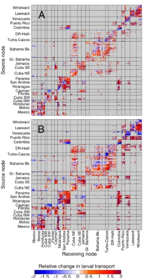
Figure 2-5: Relative change in larval transport between the surface-dwelling and OVM simulations. Entries in the relative change matrix are given by cij = _1/2(aaij_ij_+bbij_ij₎

where the aij is the larval transport for surface-dwelling larvae and bij is the larval

transport for OVM larvae. Rows within each matrix correspond to release sites (source nodes) and columns to settlement sites (receiving nodes). Red colors indicate more larvae transported in the surface-dwelling simulations, and blue colors indicate more larvae transported in the OVM simulations. Source and receiving nodes are grouped within regions, and regions are arranged roughly west to east. For a map of regions, see Figure 2-12. Two pelagic larval durations (PLD) were investigated: (A) short (20-30 d) PLD and (B) long (40-50 d) PLD.

(34)

likely to reach the neighboring regions of the Gulf of Colombia, Puerto Rico, and the Windward Islands compared with surface-dwelling larvae (Figure 2-5). Likewise, Mexican reefs were more likely to receive larvae from the northern coast of Cuba and from the Bahamas Bank under OVM simulations than surface-dwelling simulations. Relative change in larval transport between evenly-distributed and surface simu-lations (Figure 2-13) and between evenly-distributed and OVM larvae (Figure 2-14) confirm that the dispersal and transport of evenly-distributed larvae is similar to that of OVM larvae (note that Figure 2-5 and Figure 2-13 show the same regional patterns mentioned above). Evenly-distributed behavior led to slightly greater trans-port than OVM (Figure 2-14), but the changes were much smaller in magnitude than the relative diﬀerences observed between the surface-dwelling behavior and either of the deeper-dwelling behaviors (Figures 2-5 and 2-13).

2.5 Discussion

In this study, we comprehensively examined vertical distribution patterns across the larval period for various taxa of coral reef fish, finding distinct and notable diﬀerences both within and between coral reef fish families. We identified three prevalent pat-terns in the field observations: surface-dwelling, evenly-distributed, and ontogenetic vertical migration (OVM). We simulated these vertical behaviors in a biophysical model to investigate the implications for dispersal and population connectivity that arise from these innate, taxon-specific behavioral diﬀerences. By simulating five years of daily larval releases from 261 coral reef sites across the Caribbean region, we were able to evaluate the robustness of dispersal patterns across time and space.

We found that surface-dwelling fish larvae—representative of, for example, the often-abundant goatfishes and mojarras—disperse substantially longer distances than

(35)

larvae that were evenly-distributed in the upper 100 m or those that were onto-genetically migrating. The difference in the dispersal kernels between the evenly-distributed and the OVM larvae was surprisingly small. This suggests that the con-straint on dispersal distance is imposed by having some larvae spend time at depth, but an age-specific pattern of increasing depth is not required to restrict dispersal distance. The difference in dispersal distance due to changes in our focal traits, ver-tical behavior and PLD, are much greater than the differences in dispersal kernels between seasons or years. This suggests that selective forces acting on the evolution of spawning seasonality are likely due to factors other than dispersal potential (e.g., food availability, avoidance of larval predators, energy constraints on adults).

In contrast to these overall results, retention and connectivity on a regional and local (per-polygon, ca. 50 km in alongshore direction) basis showed spatial variation in which traits maximize dispersal or connectivity. Surface-dwelling larvae were as likely as deeper-dwelling larvae to be retained in Panama, Nicaragua, and Florida, while OVM and evenly-distributed larvae were more likely than surface-dwelling lar-vae to be exchanged between Cuba and the Mesoamerican reefs (Figures 2-3, 2-5, and 2-13). Surface-dwelling larvae are entrained by wind-driven circulation, predom-inantly to the northwest in the Caribbean (Tang et al., 2006). In contrast, vertically migrating larvae are more likely to be transported into the eddy field, riding the mesoscale anticyclonic gyre linking Mexico to Southwest Cuba (Kough et al., 2013; Paris et al., 2005). Other studies have found that a cyclonic gyre formed in the Gulf of Honduras drives retention and connectivity in the Mesoamerican reefs (Butler et al., 2011; Martínez et al., 2019; Tang et al., 2006). Subsurface geostrophic flows are important in the eastern Caribbean, where OVM larvae were more likely than surface-dwelling larvae to be retained in Venezuela, and transported from Venezuela to the Windward Islands (Figure 2-5). Oﬀ the coast of Venezuela, westward currents

(36)

have been observed at the surface, overlaying a subsurface eastward jet (Andrade et al., 2003; Hernandez-Guerra and Joyce, 2000). Because of the complex interaction among larval behavior, PLD, spatial variation in ocean currents, habitat availability, and seascape geomorphology, the same larval vertical behavior can lead to different dispersal and connectivity outcomes, and concomitant population effects, across re-gions. Therefore, pan-Caribbean species might have regional differences in behavior or PLD [e.g., especially in species that exhibit an extended competency period like the bluehead wrasse (Sponaugle and Cowen, 1997; Victor, 1986)], or distinct popula-tion genetic structure across regions (Kool et al., 2010; Selkoe et al., 2014; Truelove et al., 2017).

The diversity of larval vertical behaviors that we observed, and their strong ef-fect on dispersal and population connectivity in our simulations, indicates that these behaviors can play a role in coral reef fish population persistence and evolution (Sponaugle et al., 2002; Strathmann et al., 2002). Furthermore, our results shed light on how larval traits could have evolved to maximize the chance of reaching suitable settlement habitat, particularly if we consider that suitable habitat may be distributed in accordance with other traits of each species. For example, if in-traspecific competition for resources, including space, is low for adult and juvenile fish of a given species, then retention near suitable habitat—i.e. where the adults spawned—may be a successful strategy (Burgess et al., 2014; Hovestadt et al., 2001; Waser, 1985). On the other hand, if intraspecific competition is high and spawning adults are occupying habitat already at or near carrying capacity, then suitable habi-tat would be elsewhere and longer-distance dispersal would increase the probability of larvae finding suitable settlement habitat. Traits such as deeper-dwelling larvae, which restrict dispersal, can therefore facilitate local adaptation (Strathmann et al., 2002).

(37)

On the other hand, the interplay of multiple larval traits determines larval sur-vival and population persistence. In our results, surface-dwelling larvae dispersed to greater distances from their natal reef and had a higher overall probability of arriving at settlement habitat compared to deeper-dwelling larvae with the same PLD. However, life in the surface waters is likely to come with greater risks of star-vation, predation, and UV light damage. Vertical distributions of chlorophyll and zooplankton generally show a peak in the subsurface, with lower values at the very surface (Espinosa-Fuentes et al., 2009; Hopkins, 1982; Llopiz, 2008). In addition to lower food availability, larvae living in the uppermost part of the water column must contend with high light, which increases their risk of predation and requires high levels of pigmentation to protect against UV damage. Therefore, greater dispersal and connectivity seems to be the only discernable advantage to a coral reef fish of spending its entire larval duration in the surface waters.

In addition to the traits that we examine in this study, there are myriad processes that determine the successful settlement of larval coral reef fish. Larval growth rates, and therefore often the pelagic larval duration, depend on temperature and food availability (Houde, 1989). Larval mortality rates decrease with size (Houde, 1997) and will vary spatially—horizontally due to patchy predator distributions and verti-cally due to predator behaviors and light availability. While mortality rates can have important impacts on modeled population connectivity and recruitment (Cowen et al., 2006; Paris et al., 2007), true recruitment and demographic connectivity will also depend on tradeoﬀs among larval traits (e.g., behavior, growth rate, PLD, mortality) as well as adult traits (e.g., longevity, fecundity, spawning periodicity) (Cowen et al., 2006). Horizontal swimming ability increases with size and fin development (Peck et al., 2012), and larvae may use directional swimming in response to cues as they prepare to settle (Leis, 2006). Nearshore physical processes, including tides, internal

(38)

waves, and coastal boundary currents can also aﬀect larval transport and settlement (Pineda et al., 2007). As models increase in complexity, more of these processes can be incorporated. However, the strength of modeling studies lies in their ability to isolate parameters for the purposes of hypothesis testing, and we have analyzed the interaction of two larval traits—pelagic larval duration and vertical distribution behavior—to test the hypothesis that species with surface-dwelling larvae disperse further and exhibit greater population connectivity.

The experiences of planktonic larvae, from their large-scale transport in ocean currents to their small-scale movement in response to both biotic and abiotic cues, re-main diﬃcult to study. Although biological-physical modeling is one of our strongest tools for forming and testing hypotheses about larval dispersal and connectivity, there is a lack of detailed knowledge of the behaviors of many species. By probing the trait space that is defined by larval vertical behavior and PLD, we demonstrate an approach that could be used to predict the dispersal and connectivity across many taxa. Our study is limited to three vertical behaviors and two pelagic larval dura-tions, but shows the value of a trait-based analysis of dispersal and connectivity. For example, we can now predict that two species with similar larval durations, one that undergoes ontogenetic vertical migration and another that shows weak depth preferences, would be predicted to have similar patterns of dispersal, although reten-tion and connectivity may vary on a regional basis. These findings can help guide a management system that must take into account numerous species, goals, and constraints.

(39)

2.6 Supplemental Figures and Tables

Short Duration Long Duration Surface Even OVM Surface Even OVM

Winter 223 173 165 443 364 342

Spring 225 155 151 449 334 317

Summer 234 157 152 479 335 321

Fall 217 165 158 421 355 341

Table 2.1: Median dispersal distance by season. The median dispersal distance (km) of all larvae that reach settlement habitat under each behavior and duration combination, separated by the larval release season. Seasons are defined by release dates with winter covering Jan-March, spring April-June, summer July-Sept, and fall Oct-Dec. Distances are rounded to the nearest integer.

Timestep (seconds)

Update location of particles 1200

Add sub-gridscale turbulence 2400

Update particle depths to match desired vertical distribution 2400

Diﬀusivity (m2 s-1)

HyCOM Global grid 10

Gulf of Mexico grid 20

Table 2.2: Timesteps and diﬀusivity parameters used for integration of Connectivity Modeling System simulations.

(40)

Figure 2-6: The full set of family-level larval fish vertical distributions. Each set of 3 panels represents a taxon, with the name given on the left. The columns of sub-panels refer to size classes 1 through 3 that represent respectively 25, 25, and 50% of the observed size range, excluding a small number of outliers. Each sub-panel shows the proportional abundance in 4 depth bins in the upper 100 m, and each sub-panel lists the sample size in that taxon and size class.

(41)

Figure 2-7: The full set of subfamily-, tribe-, and genus-level larval fish vertical distributions. Each set of 3 panels represents a taxon, with the name given on the left. The upper three rows are genera in the family Labridae; the middle three rows are genera in the family Scaridae; the bottom three rows are two subfamilies and one tribe in the family Serranidae. The columns of sub-panels refer to size classes 1 through 3 that represent respectively 25, 25, and 50% of the observed size range, excluding a small number of outliers. Each sub-panel shows the proportional abundance in 4 depth bins in the upper 100 m, and each sub-panel lists the sample size in that taxon and size class.

(42)

Figure 2-8: Surface associated taxa and their depth in the water column. In order to show the importance of the neuston net sampling (0-1 m depth bin), we use proportional concentration (N per m3_{) instead of abundance (N per m}2_).

(a) Combined observations of OVM (b) Simulated OVM

Figure 2-9: Combined observations of ontogenetic vertical migration (OVM) and Simulated OVM. The left panel (a) shows the field observations of proportions at depth, averaged across the 5 taxa showing OVM behavior: Pomacentridae, Pomacan-thidae, Grammistini, Anthiinae, and Xyrichtys. The right panel (b) shows the OVM behavior used in model simulations, which was generated by smoothing the 4-depth distribution to a 9-depth distribution by fitting a density kernel to the 4-depth dis-tributions and then integrating that kernel within the depth bins shown in the right panel.

(43)

Figure 2-10: Seasonal dispersal kernels. Shown for short PLD (first row) and long PLD (second row) for surface-dwelling (first column), evenly-distributed (middle column) and OVM (third column) simulations. Seasons are defined by release dates with winter covering Jan-March, spring April-June, summer July-Sept, and fall Oct-Dec. All kernels are displayed on the same axes, and the sum of probabilities in each kernel (each colored curve) is equal to 1.

Figure 2-11: Annual dispersal kernels. Dispersal kernels of successfully settled larvae for combinations of larval behaviors and pelagic larval durations (PLD). (Columns) Three larval behavior simulations were conducted: surface-dwelling, evenly-distributed, and ontogenetic vertical migration (OVM). (Rows) Short and long PLD simulations correspond to 20-30 days and 40-50 days, respectively. Larvae are assigned to a year based on their release date between January 1 2004 and Decem-ber 31 2008. All kernels are displayed on the same axes, and the sum of probabilities in each kernel (each colored curve) is equal to 1.

(44)

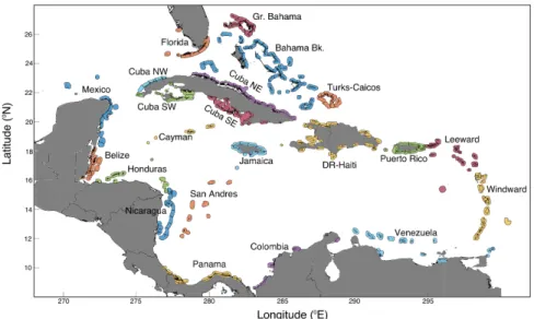
Figure 2-12: Map of coral reef habitat used in larval dispersal simulations. The Caribbean coral reefs, represented by 261 polygons, are colored by region, follow-ing Cowen et al. (2006). Region names shown here match the region names used on Figs. 3, 4, S7, S8 and S9. The regions are (roughly west to east): Mexican Caribbean and Campeche Bank (Mexico); Belize; Gulf of Honduras (Honduras); Northwest Cuba (Cuba NW); Southwest Cuba (Cuba SW); Florida Keys and west coast reefs (Florida); Cayman Islands, Rosario and Misteriosa (Cayman); Nicaraguan Rise Islands (Nicaragua); Colombian Archipelagos (San Andres); Panama and Costa Rica (Panama); Northeast Cuba (Cuba NE); Southeast Cuba (Cuba SE); Jamaica and Pedro Bank (Jamaica); Grand Bahama (Gr. Bahama); Bahamas Bank and SE Bahamas Island (Bahama Bk.); Turks and Caicos Islands (Turks-Caicos); Domini-can Republic and Haiti (DR-Haiti); Gulf of Colombia (Colombia); Puerto Rico and Mona Islands (Puerto Rico); Venezuelan Corridor, Tobago to Aruba (Venezuela); Leeward Islands (Leeward); Windward Islands (Windward).

(45)

Figure 2-13: Relative change in larval transport between the surface-dwelling and evenly-distributed simulations. Entries in the relative change matrix are given by cij = _1/2(aaij_ijb_+bij_ij) where the aij is the larval transport for surface-dwelling larvae and

bij is the larval transport for evenly-distributed larvae. Rows within each matrix

correspond to release sites (source nodes) and columns to settlement sites (receiving nodes). Red colors indicate more larvae transported in the surface-dwelling simu-lations, and blue colors indicate more larvae transported in the evenly-distributed simulations. Source and receiving nodes are grouped within regions, and regions are arranged roughly west to east. For a map of regions, see Figure 2-12. Two pelagic larval durations (PLD) were investigated: (A) short (20-30 d) PLD and (B) long (40-50 d) PLD.

(46)

Figure 2-14: Relative change in larval transport between the evenly-distributed and ontogenetic vertical migration (OVM) simulations. Entries in the relative change matrix are given by cij = _1/2(aaij_ijb_+bij_ij₎ where the aij is the larval transport for

evenly-distributed larvae and bij is the larval transport for OVM larvae. Rows within

each matrix correspond to release sites (source nodes) and columns to settlement sites (receiving nodes). Red colors indicate more larvae transported in the evenly-distributed simulations, and blue colors indicate more larvae transported in the OVM simulations. Source and receiving nodes are grouped within regions, and regions are arranged roughly west to east. For a map of regions, see Figure 2-12. Two pelagic larval durations (PLD) were investigated: (A) short (20-30 d) PLD and (B) long (40-50 d) PLD.

(47)

Chapter 3 Evidence and patterns of tuna

spawning inside a large no-take

Marine Protected Area

3.1 Abstract

1

The Phoenix Islands Protected Area (PIPA), one of the world’s largest marine pro-tected areas, represents 11% of the exclusive economic zone of the Republic of Kiri-bati, which earns much of its GDP by selling tuna fishing licenses to foreign nations. We have determined that PIPA is a spawning area for skipjack (Katsuwonus pelamis), bigeye (Thunnus obesus), and yellowfin (Thunnus albacares) tunas. Our approach included sampling larvae on cruises in 2015-2017 and using a biological-physical model to estimate spawning locations for collected larvae. Temperature and

chloro-1_{Originally published as “Hernández, C. M., Witting, J., Willis, C., Thorrold, S. R., Llopiz,}

J. K., & Rotjan, R. D. (2019). Evidence and patterns of tuna spawning inside a large no-take Marine Protected Area. Scientific Reports, 9(1), 10772. https://doi.org/10.1038/s41598-019-47161-0.” This version diﬀers only in formatting.

(48)

phyll conditions varied markedly due to observed ENSO states: El Niño (2015) and neutral (2016-2017). However, larval tuna distributions were similar amongst years. Generally, skipjack larvae were patchy and more abundant near PIPA’s northeast corner, while Thunnus larvae exhibited lower and more even abundances. Genetic barcoding confirmed the presence of bigeye (Thunnus obesus) and yellowfin (Thunnus albacares) tuna larvae. Model simulations indicated that most of the larvae collected inside PIPA in 2015 were spawned inside, while stronger currents in 2016 moved more larvae across PIPA’s boundaries. Larval distributions and relative spawning output simulations indicate that both focal taxa are spawning inside PIPA in all 3 study years, demonstrating that PIPA is protecting viable tuna spawning habitat.

3.2 Introduction

Tropical tunas are extremely valuable worldwide as a source of protein and income. Skipjack tuna alone provide approximately 50-60% of annual global tuna catches (Western and Central Pacific Fisheries Commission, 2018). Pacific island nations earn a large proportion of their gross domestic product (GDP) from tuna, many by selling fishing licenses to the commercial fleets of foreign nations to operate in their exclusive economic zones (EEZ) (Bell et al., 2013). One of these island nations is the Republic of Kiribati, which comprises 34 islands with a total land area of 810 km2 _{and an EEZ of 3.5 million km}2_{, across 3 archipelagos that span 4.7°N to}

11.4 °S and 150.2°W to 187 °W: the Line Islands, the Phoenix Islands, and the Gilbert Islands. For this low-lying ocean nation, tuna fishing by foreign commercial fleets is incredibly important to their economy: from 2006 to 2015, fishing license revenue represented 39.5% of GDP on average, ranging from 19.2% to 93.5% (GDP (Current US$) 2018; Ministry of Finance and Economic Development and Ministry

(49)

of Fisheries and Marine Resource Development, 2016). Some of the variance in fishing license revenue can be attributed to the El Niño Southern Oscillation (ENSO) cycles. El Niño conditions tend to cause skipjack tuna, which dominate the catch in Kiribati waters, to move from the western Pacific warm pool into the central Pacific, and particularly into the Phoenix Islands region (Hanich et al., 2018; Lehodey et al., 1997). The year of highest contribution of fishing licenses to GDP, 2015, was an El Niño year, and Kiribati reported fishing license revenue of USD 148.8 million (Ministry of Finance and Economic Development and Ministry of Fisheries and Marine Resource Development, 2016).

Despite heavy reliance on tuna license revenues, approximately half of the Kiribati EEZ in the vicinity of the Phoenix Islands archipelago—and 11.3% of their total EEZ—is currently a no-take marine protected area (MPA) with UNESCO World Heritage Designation. The Phoenix Islands Protected Area (PIPA) is one of the largest marine protected areas in the world at 408,250 km2_{. Created in 2008 as a}

mixed-use MPA, and closed entirely to all commercial fishing activities in January 2015, PIPA comprises 8 atolls, 2 shallow submerged coral reefs, at least 14 seamounts, and a large area of deep ocean (Rotjan et al., 2014; Witkin et al., 2016). This MPA was established to protect the many endangered and endemic species that live within its boundaries, as well as to protect the migratory birds, mammals, and sea turtles that pass through the area. Populations of previously exploited species, such as giant clam and coconut crab, have been recovering since the establishment of the MPA (Rotjan et al., 2014).

In addition to biodiversity goals, the PIPA Management Plan lays out the hope that, if well-enforced, PIPA may protect tuna breeding stocks and potential spawn-ing grounds. Although enforcspawn-ing a no-take policy in an area the size of PIPA can be diﬃcult, Automatic Identification System (AIS) data from ships indicates that

(50)

virtually all fishing activity did indeed stop after January 1, 2015 (Mccauley et al., 2016; Witkin et al., 2016). Furthermore, detected fishing days in (non-PIPA) Kiri-bati waters from AIS data actually increased from 2014 to 2015, indicating that fishing vessels moved out of PIPA but continued to fully subscribe fishing permit days for use in other parts of the Kiribati EEZ (Hanich et al., 2018; Witkin et al., 2016). With effective enforcement inside PIPA, but heavy fishing pressure outside (Mccauley et al., 2016), there may be value in protecting tuna spawning grounds, and potential for regional economic gain via “spillover effects” that may materialize once the closure has been in place long enough. Spillover effects occur when time- and/or area-closures result in increased biomass around MPA margins, which then moves outside the protected area where it can benefit fisheries, and these effects have been detected across a number of taxonomic groups and a range of MPA sizes (Di Lorenzo et al., 2016; Halpern et al., 2009; Thompson et al., 2017). For tunas in PIPA, it was assumed that fisheries protection of a large area where spawning occurs could have recruitment and biomass benefits in surrounding Kiribati waters, but tuna spawning activity within PIPA has not yet been confirmed.

Tropical tuna species that are likely to use the waters in PIPA for foraging and spawning include skipjack (Katsuwonus pelamis), yellowfin (Thunnus albacares), and bigeye (Thunnus obesus). Skipjack tuna are most abundant within 20°of the equator, but are found as far north as 40°N (Arrizabalaga et al., 2015). Yellowfin tuna are concentrated in equatorial waters and prefer temperatures above 25°C (Arrizabalaga et al., 2015). Bigeye tuna, the largest and most valuable of the tropical tunas, have a range that extends from 40°S to 40°N (Arrizabalaga et al., 2015). Albacore tuna (Thunnus alalunga) may also pass through the region, but because of its subtropical to temperate habitat preferences, this species accounts for <1% of the tuna catch in Kiribati (Ministry of Finance and Economic Development and Ministry of Fisheries