HAL Id: insu-01500417
https://hal-insu.archives-ouvertes.fr/insu-01500417
Submitted on 3 Apr 2017
HAL is a multi-disciplinary open access archive for the deposit and dissemination of sci-entific research documents, whether they are pub-lished or not. The documents may come from teaching and research institutions in France or abroad, or from public or private research centers.
L’archive ouverte pluridisciplinaire HAL, est destinée au dépôt et à la diffusion de documents scientifiques de niveau recherche, publiés ou non, émanant des établissements d’enseignement et de recherche français ou étrangers, des laboratoires publics ou privés.
regional climate system model
Philippe Drobinski, Sophie Bastin, Thomas Arsouze, Karine Beranger,
Emmanouil Flaounas, Marc Stefanon
To cite this version:
Philippe Drobinski, Sophie Bastin, Thomas Arsouze, Karine Beranger, Emmanouil Flaounas, et al.. North-western Mediterranean sea-breeze circulation in a regional climate system model. Climate Dynamics, Springer Verlag, 2018, 51 (3), pp.1077-1093. �10.1007/s00382-017-3595-z�. �insu-01500417�
North‑western Mediterranean sea‑breeze circulation in a regional
climate system model
Philippe Drobinski1 · Sophie Bastin2 · Thomas Arsouze3 · Karine Béranger4 ·
Emmanouil Flaounas5 · Marc Stéfanon6
Received: 31 July 2015 / Accepted: 19 February 2017
© The Author(s) 2017. This article is an open access publication
regional climate model (AORCM) coupling WRF and NEMO-MED12 in the frame of HyMeX/MED-CORDEX are compared. One result of this study is that these simu-lations reproduce remarkably well the intensity, direction and inland penetration of the sea breeze and even the exist-ence of the shallow sea breeze despite the overestimate of temperature over land in both simulations. The coupled simulation provides a more realistic representation of the evolution of the SST field at fine scale than the atmosphere-only one. Temperature and moisture anomalies are created in direct response to the SST anomaly and are advected by the sea breeze over land. However, the SST anomalies are not of sufficient magnitude to affect the large-scale sea-breeze circulation. The temperature anomalies are quickly damped by strong surface heating over land, whereas the water vapor mixing ratio anomalies are transported further inland. The inland limit of significance is imposed by the vertical dilution in a deeper continental boundary-layer. Keywords Air/sea interactions · Breeze · Mistral · MORCE regional climate system model · HyMeX · MED-CORDEX · ESCOMPTE
1 Introduction
The Mediterranean basin has quite a unique character that results from both physiographic and climatic conditions and historical and societal developments. Located between the midlatitude storm rainband and the Sahara Desert, the Mediterranean region experiences a profound seasonal hydrological cycle, with wet-cold winters and dry-warm summers (Peixoto et al. 1982) and a large variability at mesoscale. Indeed, the complex geography of the region, which features a nearly enclosed sea with high sea surface Abstract In the Mediterranean basin, moisture transport
can occur over large distance from remote regions by the synoptic circulation or more locally by sea breezes, driven by land-sea thermal contrast. Sea breezes play an impor-tant role in inland transport of moisture especially between late spring and early fall. In order to explicitly represent the two-way interactions at the atmosphere-ocean interface in the Mediterranean region and quantify the role of air-sea feedbacks on regional meteorology and climate, simula-tions at 20 km resolution performed with WRF regional climate model (RCM) and MORCE atmosphere-ocean
This paper is a contribution to the special issue on
Med-CORDEX, an international coordinated initiative dedicated to the multi-component regional climate modelling (atmosphere, ocean, land surface, river) of the Mediterranean under the umbrella of HyMeX, CORDEX, and Med-CLIVAR and coordinated by Samuel Somot, Paolo Ruti, Erika Coppola, Gianmaria Sannino, Bodo Ahrens, and Gabriel Jordà.
* Philippe Drobinski
philippe.drobinski@lmd.polytechnique.fr
1 LMD/IPSL, Ecole polytechnique, Université Paris-Saclay,
Sorbonne Universités, UPMC Univ., Paris 06, CNRS, Palaiseau, France
2 LATMOS/IPSL, UVSQ, Université Paris-Saclay, Sorbonne
Universités, UPMC, Univ., Paris 06, CNRS, Guyancourt, France
3 École Nationale Supérieure des Techniques Avancées/
ParisTech, Université Paris-Saclay, Palaiseau, France
4 Laboratoire d’études des Transferts en Hydrologie et
Environnement, CNRS, IRD, Grenoble INP and Université Joseph Fourier, St-Martin d’Héres, France
5 National Observatory of Athens, Athens, Greece 6 LSCE/IPSL, CEA and UVSQ, Université Paris-Saclay,
temperature (SST) during summer and fall, surrounded by very urbanized littorals and mountains (Fig. 1), plays a cru-cial role in steering airflow. The morphological complex-ity of the basin leads to the formation of intense weather phenomena, such as intense cyclogenesis (e.g. Alpert et al. 1995; Trigo et al. 1999), topographically-induced strong winds like Mistral (e.g. Drobinski et al. 2005; Guénard et al. 2005, 2006; Corsmeier et al. 2005) and Tramontane (e.g. Drobinski et al. 2001), which are companion winds blowing south from the French Mediterranean coast to the African coasts (Salameh et al. 2009). The Mediterranean Sea acts as a major source of atmospheric moisture for the atmosphere in the region which controls offshore (Luca et al. 2014; Lebeaupin-Brossier et al. 2015) and onshore precipitation (e.g. Lebeaupin et al. 2006; Lebeaupin Bro-ssier et al. 2008, 2009; Lebeaupin-Brossier et al. 2013; Berthou et al. 2014, 2015, 2016).
In the Mediterranean region, sunny weather occurs over a rather long period of the year, from spring to fall. During this period, surface heating produces a significant thermal difference between land and sea. During daytime (nighttime), land temperature exceeds (is lower than) the sea surface temperature. Such differential heating produces breeze systems which can extend over a horizontal range of 100–150 km inland (Drobinski et al. 2006) and play an important role in inland transport of moisture (Bastin et al. 2005a, 2007). The horizontal extent of the breeze circu-lation is expected to be even larger in the Southern shore of the Mediterranean region as it scales as the Rossby deformation radius, which is inversely proportional to the
Coriolis parameter (Rotunno 1983; Dalu and Pielke 1989; Drobinski and Dubos 2009; Drobinski et al. 2011). The inland penetration which controls inland moisture advec-tion and often determines the band where convecadvec-tion is triggered during warm seasons, can be modulated by inter-action with mountain slopes (Kusuda and Alpert 1983; Bastin and Drobinski 2005), channeling in local valleys (Bastin et al. 2005a, b) or by synoptic wind (Estoque 1962; Arritt 1993), and particularly by Mistral (Bastin et al. 2006) or by major urban areas (Lemonsu et al. 2006).
Breeze phenomenon has never been investigated in global climate models (GCMs), since they have gener-ally been used with too coarse horizontal grid resolution to explicitly resolve breeze circulation (i.e.>100 km). An improved knowledge of the Mediterranean hydrological cycle and its variability is needed which requires a bet-ter understanding of the mesoscale atmospheric flows like sea-breezes, which transport moisture over fairly large dis-tances. It could yield important socioeconomic benefits with respect to regional projection of global change since the largest Mediterranean cities are located near the shore.
In the context of the Hydrological cycle in the Medi-terranean Experiment (HyMeX; Drobinski et al. 2014) and the Coordinated Regional Downscaling Experiment (MED-CORDEX; Ruti et al. 2015), 10–20-km resolu-tion simularesolu-tions covering the full ERA-interim reanalysis period (1989–2008) have been performed with a number of regional climate models (RCMs) and sometimes also with atmosphere-ocean regional climate models (AORCMs). Such simulations have shown their ability to simulate coastal breezes. Indeed, Stéfanon et al. (2014) have shown the role of sea-breeze in attenuating summer heatwaves over the Mediterranean coast. However no thorough analy-sis has been undertaken on the breeze dynamics itself. The objective of this study is to take advantage of companion simulations used in atmosphere-only (RCMs) and in ocean-atmosphere coupled (AORCM) modes to address the fol-lowing question: How SST diurnal cycle simulated with AORCM modulates the main characteristics of the sea-breeze (intensity, inland extent, vertical extent) with respect to RCM and how it modifies inland moisture? The study focuses on the North-Western Mediterranean because the strong regional winds like Mistral and Tramontane modu-late the sea-surface temperature in the Gulf of Lions over time scale ranging between 1 h and few days (Lebeaupin Brossier and Drobinski 2009) which in turn affects the overlying atmospheric circulation (Fig. 1). A second rea-son is the availability of a large measurement dataset col-lected in the frame of the ESCOMPTE projet in 2001 (Cros et al. 2004; Mestayer et al. 2005) and available for model evaluation.
After the introduction in Sect. 1, the ESCOMPTE data subset used in the study, the numerical experiment
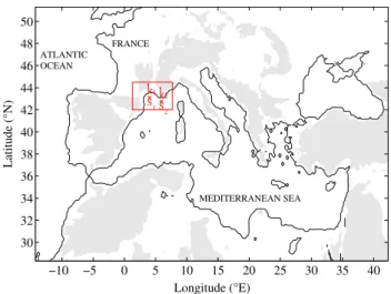
Longitude (°E) Latitude (°N) FRANCE ATLANTIC OCEAN MEDITERRANEAN SEA S1S 2 L1L 2 −10 −5 0 5 10 15 20 25 30 35 40 30 32 34 36 38 40 42 44 46 48 50
Fig. 1 Simulation domain of the HyMeX/MED-CORDEX regional
climate simulations with the shaded area indicating a topography higher than 500 m. The rectangle indicates the region of interest for this study. Locations “S1”, “S2”, “L1”, “L2” correspond to location
points at which time series of oceanic and atmospheric variables will be displayed in the present study. Subscripts “1” and “2” will be iden-tified as the “Mistral” and “Marseille” areas, respectively. Acronyms “S” and “L” stand for “Sea” and “Land”, respectively
set-up as well as the sea breeze cases are described in Sect. 2. Section 3 describes the sea surface tempera-ture pattern and variability in the two simulations and analyzes the sensitivity of the simulations to the atmos-phere/ocean coupling. Section 4 discusses the pheric response to SST differences induced by atmos-phere/ocean coupled processes. Section 5 generalizes the results to the whole ESCOMPTE data set. Section 6 concludes this study and points out some open research questions needing further investigations.
2 Data
2.1 Measurements
The study focuses on the French Mediterranean coast (see zoom in Fig. 1). Indeed, in 2001, the ESCOMPTE projet (Cros et al. 2004; Mestayer et al. 2005), was con-ducted in June and July to improve the understanding and forecast of the main flow systems (sea-breeze and valley flow) and their role in the transport of moisture and pollutants in Southern France (region shown in the zoom of Fig. 1 where the large city of Marseille and its industrialized suburbs of Fos-Berre are major sources of pollutants). Two major flow regimes alternate dur-ing summertime in this region, the Mistral and Tramon-tane northerly-northwesterly winds and the sea breeze induced by the sea land temperature contrast which advects moisture and pollutants as far as 100 km inland thus affecting the inhabitants leaving in the countryside (e.g. Bastin et al. 2007; Drobinski et al. 2007).
A large number of data were collected (meteorologi-cal data from surface weather stations, radiosondes and constant volume balloons, wind profiles from lidar, radar and sodar profilers,…; see Cros et al. 2004 for more details) and meso-scale numerical simulations performed. They allowed the analysis of the mesoscale transport and dilution by the sea-breeze, of the impact of the topography (Bastin et al. 2005a, b; Bastin and Drobinski 2005) and major urban areas (Lemonsu et al. 2006) on the sea-breeze circulation. They also allowed the analysis of the contribution of the sea-breeze to the regional transport of humidity (Bastin et al. 2005a, 2007) and pollutants (Puygrenier et al. 2005; Menut et al. 2005) and the evaluation of existing sea-breeze scaling laws with the large body of observations col-lected during the campaign (Drobinski et al. 2006). A review of the main results from this campaign can be found in Drobinski et al. (2007). Such literature ena-bles a critical evaluation of the HyMeX/MED-CORDEX simulations described hereafter.
2.2 Models and simulations
In order to explicitly represent the two-way interactions at the atmosphere-ocean interface in the Mediterranean region and quantify the role of air-sea feedbacks on regional mete-orology and climate, Drobinski et al. (2012) developed an AORCM by coupling WRF RCM and NEMO-MED12 ocean model, and hereafter referred as MORCE (model of the regional coupled Earth system). It was developed by the Institut Pierre Simon Laplace (IPSL) in collaboration with Ecole Nationale des Techniques Avancées-ParisTech (ENSTA-ParisTech), Mediterranean Institute of Oceanog-raphy (MIO) and Centre Européen de Recherche et de For-mation Avancée en Calcul Scientifique (CERFACS). This platform has been developed for process and regional cli-mate system studies, especially in vulnerable regions. The configuration used for the HyMeX/MED-CORDEX simu-lations (physical parameterizations, initial and boundary conditions) are detailed below.
2.2.1 The atmospheric and land‑surface modules
The atmospheric model is the Weather Research and Fore-casting (WRF) model of the National Center for Atmos-pheric Research (NCAR) (Skamarock et al. 2008). The domain covers the Mediterranean basin with a horizon-tal resolution of 20 km (Fig. 1). It has 28 sigma-levels in the vertical. Initial and lateral conditions are taken from the European Center for Medium-range Weather Forecast (ECMWF) ERA-interim reanalysis (Dee et al. 2011) pro-vided every 6 h with a 0.75° resolution. Moreover, to avoid unrealistic departure from the driving fields, indiscrimi-nate nudging is applied with a coefficient of 5 × 10⁻⁵ s−1 for temperature, humidity and velocity components above the planetary boundary layer (Salameh et al. 2010; Omrani et al. 2013, 2015). A complete set of physics parameteriza-tions is used with the WRF Single-Moment 5-class micro-physical scheme (Hong et al. 2004), the new Kain-Fritsch convection scheme (Kain 2004), the Yonsei University (YSU) planetary boundary layer (PBL) scheme (Noh et al. 2003) and a parameterization based on the similarity theory (Monin and Obukhov 1954) for the turbulent fluxes. The radiative scheme is based on the Rapid Radiative Trans-fer Model (RRTM) (Mlawer et al. 1997) and the Dudhia (1989) parameterization for the longwave and shortwave radiation, respectively. For the land surface, the Rapid Update Cycle (RUC) land-surface model is used (Smirnova et al. 1997).
2.2.2 The oceanic module
The numerical code for the ocean is NEMO (Madec 2008), and is used in a regional Mediterranean configuration with
a 1°/12° horizontal resolution (Lebeaupin-Brossier et al. 2011, 2012a, b). In the vertical, 50 unevenly spaced Z-lev-els are used. The vertical level thickness is 1 m in surface and nearly 4 m at 30 m depth. This eddy resolving model is referred as MED12 hereafter. The initial conditions for 3D potential temperature and salinity fields are provided by the MODB4 climatology (Brankart and Brasseur 1998) except in the Atlantic zone where the Levitus et al. 2005 clima-tology is applied. The water exchanges with the Atlantic Ocean are parameterized with a 3D relaxation to this cli-matology between 11°W and 6°W. The runoffs and the Black Sea water input are prescribed from a climatology as precipitation (Beuvier et al. 2010). The vertical diffu-sion is performed by the standard turbulent kinetic energy model of NEMO and in case of instabilities a higher dif-fusivity coefficient of 10 m2 s−1 is used. The coupling con-sists in sea surface temperature (SST) and heat (solar and non-solar), water and momentum fluxes exchanges between the two models. The 3-hourly exchanges frequency and the fields interpolation are managed via the OASIS coupler (Valcke 2006).
2.2.3 Simulations
The simulations performed with WRF RCM and MORCE AORCM, cover the ERA-interim period between 1 January 1989 and 31 December 2012 and the simulation domain is shown in Fig. 1. Two simulations are hereafter examined: • The downscaled ERA-interim reanalyses (1989–2008)
by WRF RCM is named CTL hereafter and has been evaluated in-depth over the land surrounding the Medi-terranean Sea (Claud et al. 2012; Flaounas et al. 2013; Stéfanon et al. 2014). The CTL simulations is forced by the ERA-interim SST at its lower boundary over the Mediterranean Sea.
• The downscaled ERA-interim reanalyses (1989–2008) by MORCE AORCM is named CPL and has been eval-uated in-depth for precipitation, evaporation and wind speed over the Mediterranean Sea (Claud et al. 2012; Lebeaupin-Brossier et al. 2015). The CPL simulations is forced by the NEMO-MED12 SST at its lower bound-ary over the Mediterranean Sea.
At this point, it is important to stress that other RCM and AORCM simulations have been performed in the frame of HyMeX/MED-CORDEX program. However, a multi-model approach is not possible here as the numerical set-ups are much too different between the various simula-tions for a straightforward comparison. Indeed all the other AORCM simulations but one are not nudged (Drobinski et al. 2016). In nudged CTL and CPL simulations, the same model and hence the same physics are used so the effect
of SST bias and air-sea feedbacks is isolated without any interference with other sources of error and uncertainty propagation, all other things being equal. Also, by con-straining the large-scale field, the nudged simulations being from RCM and AORCM, have the spatial and temporal variability which allow a point to point, instant to instant comparison between the simulations. Finally, the only other nudged simulation is that performed by CNRM with a horizontal resolution of 50 km which considerably lim-its the simulation of the breeze. Their “CTL” simulation uses a monthly averaged ERA-interim SST field (instead of 3-hourly in the MORCE plateform), and their “CPL” simu-lation uses a daily time step coupling (instead of 3-hourly in the MORCE plateform). For these reasons, this sensitv-ity study only uses one single model.
2.3 Brief description of the sea breeze cases
In this article, we focus on the northwestern Mediterranean area between 21 and 26 June 2001 (see zoom in Fig. 1). This period corresponds to the second intensive observa-tion period (IOP) of the ESCOMPTE campaign, which has been the most investigated period of the ESCOMPTE cam-paign as it basically covers all breeze situations that occur in this region. This period, referred as IOP2, has been split into two contiguous parts since meteorological conditions changed significantly on 23 June at 1700 UTC. The first period, hereafter called P1 (21–23 June) corresponds to the end of a Mistral situation with a moderate northwesterly to westerly wind, clear skies, hot temperature (>30 °C). The sea-breeze breaks through during the day but penetrates inland over a short distance (50 km) due to the frontal convergence with the Mistral from the north (Bastin et al. 2006; Drobinski et al. 2006). The second period, hereafter called P2 (24–26 June) best characterizes the most usual sea-breeze circulation configuration. During these three windless days, temperatures were hot (>34 °C) and the sea-breeze penetrated over a horizontal distance reaching 100–150 km (Bastin et al. 2005a, b; Drobinski et al. 2006).
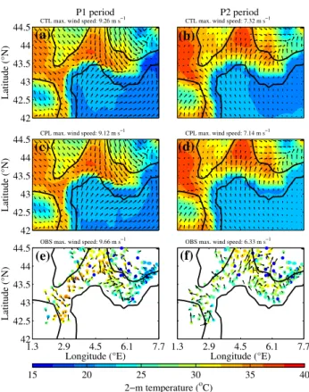
The surface flow pattern from the CTL and CPL simu-lations and from surface weather stations measurements is shown in Fig. 2 which displays the surface temperature (at 2-m height) and wind fields (at 10-m height) averaged over the P1 and P2 periods at 1800 UTC. Indeed, Bastin et al. (2005a, b), Bastin and Drobinski (2006) and Drob-inski et al. (2006) show that in this area, the maximum inland penetration of the sea breeze is often found around 1600–1800 UTC, which coincides with the maximum of the diurnal temperature cycle (note that the local solar time which is a relevant time coordinate for breeze stud-ies corresponds to universal time coordinate (UTC)+ 20 min; because of this small difference, we use the UTC time unit). The sea breeze front location corresponds to
the location of the temperature maximum or/and (when it exists) the area where the wind reverses from the south (sea breeze flow) to the north. Figure 2 reveals differences in the surface temperature and wind field patterns between the CTL and CPL simulations, and between the simulations and the measurements. These differences will be discussed in the next sections.
During the P1 period (Fig. 2a, c, e), the sea breeze blows in the Marseille area (see point L2 in Fig. 1) where it takes a westerly direction because it combines with the Mistral. The simulations shows a 2-m temperature maximum in the Rhône valley at around 43.8°N where the sea breeze and the Mistral collide. This corresponds to an inland penetra-tion of about 50 km in the Rhône valley, in good agreement with measurements of surface temperature and wind fields (Fig. 2; see also Table 2 in Drobinski et al. 2006), despite the large positive bias of the simulated temperature (about +3 °C maximum) and a weak negative wind bias (−0.4 m s−1) (Fig. 2). The Mistral is easily discernable with wind speed up to about 9 m s−1 and a pronounced northerly to northwesterly direction. The very small penetration of the
sea breeze front is due to the offshore Mistral wind which inhibits the inland progress of the sea breeze (Bastin et al. 2006) and affects moisture transport (Bastin et al. 2007). During the P2 period, the surface wind and temperature fields clearly show the sea breeze establishment and the front location in a large region in the Rhône valley (between 44.0 and 44.5°N) where there is no temperature gradient (Fig. 2b, d). The sea breeze front thus penetrates inland over a horizontal range of about 100–150 km in the Rhône valley which is also in agreement with the measurements (Fig. 2; see also Table 2 in Drobinski et al. 2006) and scal-ing laws which predict the typical horizontal extent to be of the order of the Rossby deformation radius ziN∕f ∼ 100 km (with zi∼ 1 km the atmospheric boundary layer depth,
N∼ 10−2 s−1 the Brunt-Väisälä frequency and f ∼ 10−4 s−1 the Coriolis parameter at about 45° latitude; see Rotunno 1983; Dalu and Pielke 1989; Drobinski and Dubos 2009; Drobinski et al. 2011). However, both the CTL and CPL simulations still overestimate significantly the onshore sur-face air temperature by nearly +5 °C (Fig. 2).
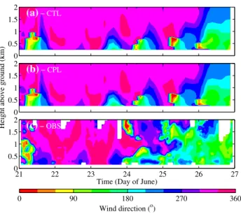
The time variability of the wind speed as a function of height is analyzed over land in the “Marseille” area (location L2 in Fig. 1) in Figs. 3 and 4 which respec-tively display the vertical profiles of the wind speed and direction from the CTL and CPL simulations and from a UHF radar wind profiler. Figures 3 and 4 clearly show the differences and the transition between the P1 and P2 periods. During the P1 period (21–23 June), the wind direction is north-northwesterly from the ground up to 2 km between 0000 and 1200 UTC. In this layer, the wind speed ranges from 5 m s−1 near the ground and can reach
Latitude (°N)
(a)
CTL max. wind speed: 9.26 m sP1 period −1
42 42.5 43 43.5 44 44.5 Latitude (°N) (c)
CPL max. wind speed: 9.12 m s−1
42 42.5 43 43.5 44 44.5 1.3 2.9 4.5 6.1 7.7 42 42.5 43 43.5 44 44.5 Latitude (°N) Longitude (°E) (e)
OBS max. wind speed: 9.66 m s−1
(b)
CTL max. wind speed: 7.32 m sP2 period −1
(d)
CPL max. wind speed: 7.14 m s−1
2−m temperature (oC)
15 20 25 30 35 40
1.3 2.9 4.5 6.1 7.7
(f)
OBS max. wind speed: 6.33 m s−1
Longitude (°E)
Fig. 2 2-m temperature (color) and 10-m wind (arrows) field
aver-aged over the P1 period (21–23 June 2001) (left column; a, c, e) and the P2 period (24–26 June 2001) (right column; b, d, f) at 1800 UTC from CTL (upper row, a, b) and CPL (middle row, c, d) simulations, and from the Météo-France surface weather stations measurements (lower row, e, f). The thick lines indicate the coastline and the 500-m height topography (a) − CTL 0 0.5 1 1.5 2
Height above ground (km)
(b) − CPL 0 0.5 1 1.5 2
Time (Day of June)
(c) − OBS 21 22 23 24 25 26 27 0 0.5 1 1.5 2 Wind speed (m s−1) 0 6 12 18
Fig. 3 Time-vs-height plots of wind speed in the “Marseille” area at
location L2 (Fig. 1) from the CTL (a), CPL (b) simulations, and from
12–15 m s−1 at 1-km height and above. These simulations in good agreement with observations provide evidence that the whole layer between the surface and 2 km is affected by the Mistral, which intensity is weaker near the surface because of the friction. During the afternoon, two different layers are apparent. In a layer between the sur-face and about 600 m above ground, the wind direction is westerly-southwesterly, associated with wind speeds of about 5–8 m s−1. In a second layer between 600 m and 2 km, the wind direction is again north-northwesterly, associated with an intensity of 7–12 m s−1. The exist-ence of these two layers indicates the onset of the sea breeze in the afternoon (i.e., at about 1100 UTC on 21 June, at about 1500 UTC on 22 June, and at about 1300 UTC on 23 June) near the coastline that lifts the Mistral up to 700 or 800 m. The low-level wind direction shift in the afternoon is present but less marked in the CTL and CPL simulations, which can in part be attributed to the too coarse vertical resolutions of the models. How-ever, the wind speed variability is much more accurately simulated even though it is slightly underestimated in the simulations (about −3 m s−1 around 1.5 km height). The weakness of the Mistral during this period allows the sea breeze to break through near the coastline where the temperature gradient between land and sea is maxi-mum (Fig. 2). Thus, during the P1 period, the Mistral that blows near the surface during nighttime is not strong enough to inhibit the sea breeze (Arritt 1993; Bastin et al. 2006) and is replaced by a sea-breeze flow near the sur-face during the afternoon.
The transition between the P1 and P2 periods occurs during the afternoon of 23 June, when the Mistral
weakens. During the P2 period, the diurnal cycle is not as well marked as during the P1 period in the observations because of the instrumental noise. The wind systems alternate between nocturnal katabatic flow combined with land breeze and diurnal anabatic flow combined with sea-breeze which typically blow between 2 m s−1 at night and 4 m s−1 during daytime (Bastin and Drobinski 2005). Such values are consistently with scaling laws (Walsh 1974; Rotunno 1983; Niino 1987; Steyn 1998; Dalu and Pielke 1989; Steyn 2003; Drobinski and Dubos 2009; Drobinski et al. 2011). The typical 2 m s−1 diurnal ampli-tude is more difficult to capture in the observations than in the simulations which simulate a much clearer diurnal cycle with typical nighttime wind speed of 1–2 m s−1 and daytime of 4–5 m s−1. In the UHF radar observations the wind speed is quasi homogeneous with height. It is also the case in the simulation during daytime, whereas dur-ing nighttime, it increases from 1–2 m s−1 in the first kilo-meter (sea-breeze depth) to 4–5 m s−1 above. The wind direction also shows the existence of a diurnal cycle near the surface within several layers: up to about 300–400 m, the wind alternates between westerly during daytime and easterly during nighttime, perpendicularly to the actual coastline. It blows up to about 1 km (sea-breeze depth) from south-westerly during daytime to north-easterly during nighttime and then veers to north-westerly above. The simulations also display a marked diurnal cycle but because of the “coarser” topography representation, the wind direction shifts between north-westerly during nighttime and south-easterly during daytime up to about 300–400 m, perpendicularly to the model coastline. It then shifts between southerly during daytime to northerly during nighttime. As in the observations, the wind direc-tion also veers to north-westerly above 1 km.
The vertical variation of the wind direction corresponds to the co-existence of a shallow sea breeze which blows from the surface up to about 400 m below a deep sea-breeze which blows above up to about 1 km (Bastin and Drobinski 2006; Lemonsu et al. 2006). Similarly to what Banta (1995) showed experimentally, two sea breezes do occur on two different depths and timescales: (1) a local-scale temperature contrast close to the shoreline, which has a pattern correlated to the coastline shape, drives a shallow sea breeze blowing perpendicularly to the local coastline; (2) a larger-scale temperature contrast drives a deeper sea breeze blowing from the south (the isotherms have a pre-dominant east-west orientation) that develops later in the day. On the contrary to Banta (1995) who observed that, by late afternoon, the shallow sea breeze blended into the deeper sea-breeze layer and was no longer evident, Bastin and Drobinski (2006) found that the shallow sea breeze persists all day long since the directions of the shallow and deep sea breezes are distinct in this region of complex coast (a) − CTL 0 0.5 1 1.5 2
Height above ground (km)
(b) − CPL 0 0.5 1 1.5 2
Time (Day of June)
(c) − OBS 21 22 23 24 25 26 27 0 0.5 1 1.5 2 Wind direction (o) 0 90 180 270 360
shape. Because of the background synoptic wind which varies during the P2 period, the deep sea breeze direction also evolves. On 24 June, the synoptic situation induces a north-westerly flow in this second layer. On 25 June, dur-ing the day, the wind has a southerly direction, which is not well captured by the simulation above 1.5 km. During the night and in the morning, this deep sea breeze does not exist and a westerly flow blows. On 26 June, the synoptic wind blows from the east. It has been shown that, on 26 June the low-level air mass, up to 2 km above ground, skirts the Mediterranean coast over land from the east-southeast (Lemonsu et al. 2006).
3 SST analysis in the CTL and CPL regional climate simulations
The sea-breeze circulation is primarily driven by a thermal contrast between land and sea, which is thus over the sea, in part controlled by the SST. In this section, we thus investi-gate the impact on the SST field of air/sea feedbacks in the CPL simulation and compare it to that from the CTL simu-lations and the observations.
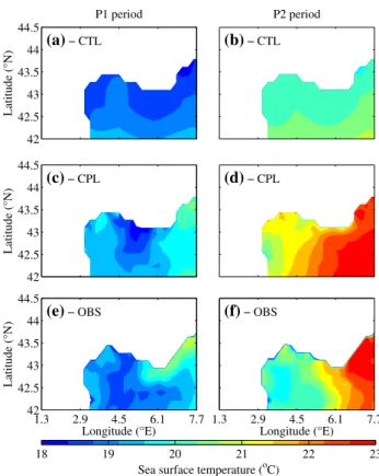
3.1 Spatial pattern of the SST fields
Figure 5 shows the SST field averaged over the P1 and P2 periods from the CTL and CPL simulations and from the observations. More precisely, the SST observations are SST products optimally interpolated which have been produced in near-real time from direct assimilation in MFSTEP large scale model (OPA-MED16) of the AVHRR Pathfinder SST from the NASA/NOAA satellites. Original satellite data are available daily with a 4 km resolution. The optimally interpolated SST product finally covers the Mediterranean basin at 1°/16° resolution, dating back to 1985, and accu-rately represents the Mediterranean SST when compared to in-situ measurements on board buoys, drifters or volun-tary observing ships, and to ARGO profilers. The satellite data, the optimal interpolation scheme and the validation of the MFSTEP optimally interpolated SST product are fully described in Marullo et al. (2007). For the P1 period, Fig. 5 shows a cool SST plume visible at the exist of the Rhône valley and directly linked to the weak Mistral blow-ing between 21 and 23 June 2001 (Fig. 2a–c). It is present in the CTL and CPL simulations and in the observations but the fine scale structure is more accurately reproduced in the CPL simulation (Fig. 5b, c). Indeed, the Mistral, chan-neled in the Rhône valley, becomes a narrow streak jet over the Mediterranean Sea. The SST is directly modulated by the wind which enhances significantly the energy loss by the sea and the SST pattern is highly correlated with the wind pattern above (e.g. Lebeaupin Brossier and Drobinski
2009). Due to a still fairly coarse horizontal resolution of the interim reanalysis (about 75 km), the ERA-interim wind speed is too smooth and weak during the Mis-tral event and therefore, the SST of the CTL simulation is also too smooth and warm at the exit of the Rhône valley (Fig. 5a, c). Elsewhere, the ERA-interim SST displays a significant cold bias with respect to the observations. The CPL simulation displays a more realistic SST field (Fig. 5b, c) but underestimates the SST along the Liguro-Provencal current, east of the Rhône valley exit (−0.7 to −0.5 °C) and overestimates the SST further south (+0.5 to +0.7 °C).
During the P2 period, the SST warms up everywhere due to a much weaker wind (Fig. 2c, d), a stronger down-ward solar flux, and to the shallow oceanic mixed layer depth which favors a fast response to any change of the atmospheric forcing. The cold SST anomaly however remains due to the trapping by the oceanic cyclonic gyre in the Gulf of Lions (e.g. Lebeaupin-Brossier et al. 2013). The signature of the preceding Mistral event on the SST pattern is however smoothed and damped due to SST redistribution by the regional oceanic circulation. During this period, the SST underestimation of the CTL simulation is even more striking than during the P1 period (21–23 June 2001), espe-cially east of 5°E (about −2 °C) and the SST pattern is too
Latitude (°N) P1 period (a) − CTL 42 42.5 43 43.5 44 44.5 Latitude (°N) (c) − CPL 42 42.5 43 43.5 44 44.5 Latitude (°N) Longitude (°E) (e) − OBS 1.3 2.9 4.5 6.1 7.7 42 42.5 43 43.5 44 44.5 (b) − CTL P2 period (d) − CPL
Sea surface temperature (oC)
18 19 20 21 22 23
(f) − OBS
Longitude (°E) 1.3 2.9 4.5 6.1 7.7
Fig. 5 SST field averaged over the P1 period (upper row; a–c) and
the P2 period (lower row; d–f) from CTL (left column, a, d) and CPL (middle column, b, e) simulations and from satellite observations (right column, c, f)
homogeneous and smooth (Fig. 5d, f). The east-west SST gradient is present in the CPL simulation with however a too warm SST in the region of the persisting cold anomaly (+1°) and a fairly accurate value of SST east of 5°E.
The modifications of the SST due to atmosphere/ocean coupling are visible over the whole investigated domain and therefore at a distance of typically 100 km from the shore where they can affect the atmospheric response and the land-sea breeze system (Rotunno 1983; Drobinski and Dubos 2009).
3.2 SST variability
The ERA-interim SST reanalysis is provided to WRF RCM on a daily basis. Even though the heat capacity of water is much higher than that of air, the diurnal evolution of SST might have an influence on the breeze circulation. Figure 6 shows time series of SST averaged over the Mediterranean Sea in the zoom of Fig. 1 and at two different locations: • at 3.62°E/42.50°N in the cold SST anomaly produced
by the Mistral during the P1 period (21–23 June 2001) (see point S1 in Fig. 1)
• at 5.52°E/42.15°N, south of Marseille, in a region where the CTL SST is colder than the CPL SST (see point S2 in Fig. 1).
In ERA-interim reanalysis, we clearly see the absence of SST variation at a frequency higher than the diurnal fre-quency. The ERA-interim SST displays a stair-like shape (Fig. 6). Conversely, the 3-h coupling in the CPL simula-tion allows the simulasimula-tion of the diurnal variasimula-tion of the SST (Fig. 6).
In the “Mistral” area (point S1), the ERA-interim (CTL) SST is slightly warmer than the CPL SST but is within the diurnal variation range of the CPL SST. As the Mis-tral weakens, the SST increases but at a much slower rate in the CTL simulation with respect to the CPL simulation. It, however, remains within the diurnal variation range of the CPL SST until 25 June. Conversely, in the “Marseille” area (point S2), the ERA-interim (CTL) SST is much colder than the CPL SST and always outside of the diurnal vari-ation range of the CPL SST. The SST difference increases
significantly after 24 June reaching 3 °C on the night of 26–27 June. The fact that CPL SST remains closer to CTL SST in the “Mistral” area can be attributed to the cyclonic oceanic circulation in the Gulf of Lions which traps the cold water mass produced by the Mistral event and prevents its advection and dilution. The trapping of the cold water mass exists in the ERA-interim reanalysis even though it spreads horizontally over a too large area. The presence of the persisting cold water mass explains why there is a better agreement between the CPL and CTL SSTs in the “Mis-tral” area than in the “Marseille” area. The coupling how-ever produces a more accurate pattern with more realistic meso-scale structures and time variation. Figure 6 shows that the coupling produces a SST minimum around 1200 UTC and a SST maximum shortly before 0000 UTC. SST is thus almost 6 h behind the near-surface air temperature, most probably due to the low thermal diffusivity of water.
Figure 7 displays the standard deviation 𝜎𝛿SST of the CPL–CTL SST difference over P1 and P2 periods. The standard deviation quantifies the spatial variability of the difference between the two SSTs. During P1 period, when the average bias between the two simulations is the lowest, the value of the standard deviation can be mainly attributed to the diurnal cycle.
In detail, the zone of highest variability south of 42.5°N along the Spanish coast, is due to the shrinking of the cold SST anomaly produced at night by the Mistral blowing over the sea. The Mistral is the strongest on 22 June and weakens
Fig. 6 SST time series from
CTL (ERA-interim SST; solid
line) and CPL (dashed line)
simulations in a the “Mistral” area (S1 location), b the “Mar-seille” area (S2 location) and c averaged over the whole domain (rectangle in Fig. 1) 21 22 23 24 25 26 27 17 19 21 23 25
Time (day of June)
SST (°C) "Mistral" area (S1) (a) CTL CPL 21 22 23 24 25 26 27 Time (day of June)
"Marseille" area (S2)
(b)
21 22 23 24 25 26 27 Time (day of June)
Domain average (c) Longitude (°E) Latitude (°N) (a) P1 period 1.3 2.9 4.5 6.1 7.7 42 42.5 43 43.5 44 44.5 Longitude (°E) P2 period (b) 1.3 2.9 4.5 6.1 7.7 σδSST (°C) 0 0.4 0.8 1.2
Fig. 7 Standard deviation of the CPL–CTL SST difference 𝜎𝛿SST over P1 (a) and P2 (b) periods
until 24 June. The shallow ocean mixed layer favors a rapid response to daytime heating. The surface water warms up in the region where the Mistral weakens the most, i.e. far south from the French coast. It is visible in Fig. 8 which displays the evolution of the SST spatial pattern from CTL and CPL simulations and from satellite observations during the P1 period. The CTL simulation produces a SST field with a north-south gradient. The SST is in general colder north of the domain along the French Mediterranean coast. Between 21 and 23 June, the SST warms quasi uniformly by about 1.5–2 °C. The CPL simulation produces a north-south oriented cold streak along the Rhône valley axis which warms up and shrinks between 21 and 23 June. The observed SST also displays a cold streak which however warms up at a much lower rate and also extends to the east, south of the domain. So outside the region of influence of the Mistral, south of the French coast, the CPL—CTL SST difference is mainly driven by the simulation of the diurnal cycle in the CPL simulation. The variability 𝜎𝛿SST ∼ 0.5◦ C is mostly due to the diurnal cycle. It increases up to 0.7 °C in the region where the cold anomaly trapped within the oceanic cyclonic gyre reduces its horizontal extent.
During the P2 period, the value of 𝜎𝛿SST increases up to 1.0 °C and is maximum south of Marseille (see S2 in Fig. 1). It is caused by the representation of the diurnal cycle and to the stronger warming in the CPL simulation with respect to the CTL simulation. Figure 9 shows larger differences between CTL and CPL simulations, and the sat-ellite observations. In the CTL simulation, the SST pattern is very similar to that of the P1 period but is much warmer.
In the CPL simulation and satellite observations, region of influence of the Mistral remains cooler and warms up at lower rate than further east. Such persisting cold anomaly is due to the cyclonic gyre trapping in the Gulf of Lions. In the east of the domain, the SST warms up quickly (3 °C between 24 and 26 June). It is well reproduced in the CPL simulations but it spreads too far west. If we con-sider that 0.5 °C variability corresponds to the SST diurnal cycle, then another 0.5 °C can be attributed to the SST drift between the two simulations during the P2 period.
4 Atmospheric response to SST in the CTL and CPL regional climate simulations
In this section we investigate the difference of the atmos-pheric responses induced by the SST anomalies between the CTL and CPL simulations. Between 21 and 24 June, the CPL SST is cooler at night and warmer during daytime with respect to ERA-Interim SST. This SST difference impacts directly the temperature of the overlying air and thus the land/sea thermal contrast. Figure 10 displays the evolution of the 2-m temperature over land and over sea in the “Mistral” and the “Marseille” areas from the CTL and CPL simulations. As discussed above, the 2-m temperature over the sea is significantly affected by air/sea coupling. It is however not the case over land, where near-surface air temperature is dominantly controlled by local surface sen-sible heat flux which are high in the region in summer. Indeed, differences between CTL and CPL 2-m temperature are the highest in the middle of the day and never exceed
Latitude (°N) CTL (a) 42 42.5 43 43.5 44 44.5 CPL (b) OBS (c) Latitude (°N) (d) 42 42.5 43 43.5 44 44.5 (e) (f) (g) Longitude (°E) Latitude (°N) 1.3 2.9 4.5 6.1 7.7 42 42.5 43 43.5 44 44.5 Longitude (°E) (h) 1.3 2.9 4.5 6.1 7.7
Sea surface temperature (oC)
17 18 19 20 21 22 23 24 25
(i)
Longitude (°E) 1.3 2.9 4.5 6.1 7.7
Fig. 8 SST field from CTL (left column, a, d, g) and CPL (middle
column, b, e, h) simulations and from satellite observations (right column, c, f, i) on 21 (upper row, a–c), 22 (middle row, d–f) and 23
June (lower row, g–i)
Latitude (°N) CTL (a) 42 42.5 43 43.5 44 44.5 CPL (b) OBS (c) Latitude (°N) (d) 42 42.5 43 43.5 44 44.5 (e) (f) (g) Longitude (°E) Latitude (°N) 1.3 2.9 4.5 6.1 7.7 42 42.5 43 43.5 44 44.5 Longitude (°E) (h) 1.3 2.9 4.5 6.1 7.7
Sea surface temperature (oC)
17 18 19 20 21 22 23 24 25
(i)
Longitude (°E) 1.3 2.9 4.5 6.1 7.7
Fig. 9 Same as Fig. 8 on 24 (upper row, a–c), 25 (middle row, d–f) and 26 June (lower row, g–i)
few tenths of a degree. On average, in the “Mistral” area over the sea, the CTL and CPL 2-m temperature are similar until 24 June only differing by the diurnal amplitude due to the SST diurnal cycle in the CLP simulation. After 24 June, the two time series depart from each other (the CPL 2-m temperature being about 1 °C warmer on 25 and 26 June than the CTL 2-m temperature). In the “Marseille” area, a similar behaviour is found until 24 June. However, the difference between the CTL and CPL 2-m temperature is much larger after 24 June than in the “Mistral” area. It reaches on average 2 °C with a peak of more than 3 °C dur-ing the night of 27 June. The effect of air/sea coupldur-ing also tends to increase the diurnal variability of the near-surface air temperature over the sea. Indeed, the surface heat flux is a function of the temperature difference between the sea surface and the overlying air. With a constant SST during the day, the relaxation of the air temperature towards the constant SST produced by the flux parameterization damps the air temperature variation. The air temperature variation is only controlled by the diurnal variation of the net radia-tive flux. When air/sea coupled processes are accounted for, the diurnal variation of the SST amplifies the atmospheric response. On average, the difference is typically −0.5 and +0.5 °C at sunrise and sunset, respectively, but can reach 2 °C in magnitude after 24 June in the “Marseille” area. The land-sea contrast is thus modified between CTL and CPL simulations (Fig. 10c, d). It is computed as the difference between the 2-m temperature between L1 and S1 for the “Mistral” area and between L2 and S2 for the “Marseille” area. This figure shows that in the absence of coupling, the
diurnal amplitude of the thermal contrast reaches about 12 °C, whereas it is about 10% larger when air/sea coupling is accounted for (it can even reach 20% between 24 and 26 June in the “Marseille” area).
How these 10% additional thermal contrast impact the sea-breeze circulation is one key question. Figure 11 shows the near surface wind speed and direction from the CTL and CPL simulations at the “Mistral” and “Marseille” areas. The only visible differences are over the sea during the P2 period and are larger in the “Marseille” area than in the “Mistral” area, consistently with the near-surface air temperature difference. Conversely, over land, as for the temperature, there is no visible impact of the SST anoma-lies on the wind speed. The 10% additional thermal con-trast is too localized and of too weak magnitude to affect significantly the sea-breeze circulation at large scale.
What happens over the sea is similar to the local atmos-pheric response to fine oceanic thermal front which gen-erate thermal winds over the sea (Giordani and Planton 2000). The magnitude of SST anomalies produces local but significant modifications of the offshore wind. The modifi-cation of the offshore wind speed can reach 20% during the P2 period in the “Marseille” area but does not extend over large distance.
The modification of the offshore wind speed can reach 20% during the P2 period in the “Marseille” area but this modification is confined to the streak thermal anomaly of few tens of kilometers size. Such confined response is simi-lar to what would be expected for an oceanic thermal fron,
17 22 27 32 37 T at 2 m (°C) "Mistral" area (S1 ; L1) (a) Solid: CTL
Dashed: CPL Red: LandBlack: Sea
"Marseille" area (S2 ; L2) (b) 21 22 23 24 25 26 27 −15 −10 −5 0 5
Time (day of June)
∆
T land/sea
at 2 m (°C)
(c)
21 22 23 24 25 26 27 Time (day of June)
(d)
Fig. 10 Upper row Evolution of 2-m temperature over land (red line)
and over sea (black line) in the “Mistral” (a) and the “Marseille” (b) areas from the CTL (solid line) and CPL (dashed line) simulations.
Lower row Evolution of the land/sea thermal contrast in the
“Mis-tral” (S1–L1) (c) and the “Marseille” (S2–L2) (d) areas from the CTL
(solid line) and CPL (dashed line) simulations
0 2 4 6 8 10 WS at 10 m (m s −1 ) "Mistral" area (S1 , L1) (a) Solid: CTL Dashed: CPL Red: Land Black: Sea "Marseille" area (S2 , L2) (b) 21 22 23 24 25 26 27 0 90 180 270 360
Time (day of June)
∆
T land/sea
at 2 m (°C)
(c)
21 22 23 24 25 26 27 Time (day of June)
(d)
Fig. 11 Upper row Evolution of 10-m wind speed over land (red
line) and over sea (black line) in the “Mistral” (a) and the “Marseille”
(b) areas from the CTL (solid line) and CPL (dashed line) simula-tions. Lower row Evolution of 10-m wind direction over land (red
line) and over sea (black line) in the “Mistral” (c) and the “Marseille”
(d) areas from the CTL (solid line) and CPL (dashed line) simula-tions
it is significant in magnitude but does not extend over the typical 100–150 km distance expected for the large-scale sea-breeze.
To analyze more thoroughly the atmospheric response to the SST anomaly, we consider the evolution of the tempera-ture anomaly of CPL relative to CTL in the lowest model layers which is given by the following equation:
Similar equations can be written for water mixing ratio and wind components. Figure 12 displays the standard devia-tions 𝜎𝛿T2 of the CPL–CTL 2-m temperature difference over the P1 and P2 periods. The 2-m temperature difference variability 𝜎𝛿T2 over the sea shows a strong correlation with
𝜎𝛿SST (i.e. 0.58 and 0.75 for the P1 and P2 periods,
respec-tively). During the P1 period, the temperature anomaly variability penetrates inland in the “Marseille” area over a distance corresponding to one grid cell only. Even though we are at the limit of sensitivity with regards to the pen-etration distance, it remains consistent with observations or simulations performed at kilometer scale horizontal reso-lution (Bastin and Drobinski 2006). The presence of the Mistral does not allow sea-breeze inland penetration in the
(1)
𝜕T
CPL−CTL
𝜕t = − u⏟⏞⏞⏞⏞⏞⏞⏞⏟⏞⏞⏞⏞⏞⏞⏞⏟CTL∇TCPL−CTL
Advection of T anomalies (term I)
− uCPL−CTL∇TCTL
⏟⏞⏞⏞⏞⏞⏞⏞⏟⏞⏞⏞⏞⏞⏞⏞⏟
Advection of T by wind anomalies (term II)
− uCPL−CTL∇TCPL−CTL
⏟⏞⏞⏞⏞⏞⏞⏞⏞⏞⏞⏞⏟⏞⏞⏞⏞⏞⏞⏞⏞⏞⏞⏞⏟
Advection of T anomalies by wind anomalies (term III)
+ HFCPL−CTL
⏟⏞⏞⏞⏟⏞⏞⏞⏟
Turbulent heat flux anomalies (term IV)
Rhône valley delta. During the P2 period, no adverse wind prevents inland penetration of the sea-breeze. The largest penetration occurs along the Rhône valley axis as no moun-tain surrounding the Mediterranean coast prevents inland penetration (Bastin et al. 2005a, b). During the P2 period, most of the temperature anomaly variability penetrates over land in the “Mistral” area and not in the “Marseille” area.
Surprisingly, Fig. 13 which is similar to Fig. 12 for the wind speed anomaly, does not exhibit a similar spatial pat-tern as in Fig. 12. The largest variability is found over the sea where the perturbation by the SST anomaly is the larg-est, but over land, there is no significant effect of the SST difference on the wind speed anomaly, or in other words on the onshore penetration of the sea-breeze. From Eq. (1), this suggests that the advection of T anomalies (term I) dominates over the advection of T by wind anomalies (term II). The advection of T anomalies by wind anomalies (term III) is strongly non linear and of much lower magnitude than terms I and II. The turbulent heat flux anomalies (term IV) are totally negligible as the heat fluxes are very large over land and are not modulated by any inland advection of temperature anomaly. The large surface heat fluxes over
Latitude (°N) Longitude (°E) (a) P1 period 1.3 2.9 4.5 6.1 7.7 42 42.5 43 43.5 44 44.5 Longitude (°E) P2 period (b) 1.3 2.9 4.5 6.1 7.7 σδT 2 (°C) 0 0.3 0.6 0.9
Fig. 12 Significant standard deviation of the CPL–CTL 2-m
temper-ature difference during the P1 period (a) and the P2 period (b)
Latitude (°N) Longitude (°E) (a) P1 period 1.3 2.9 4.5 6.1 7.7 42 42.5 43 43.5 44 44.5 Longitude (°E) P2 period (b) 1.3 2.9 4.5 6.1 7.7 σδU 10 (m s−1) 0 0.3 0.6 0.9
land also explain why the temperature anomaly is not seen further inland. Indeed, the large heat fluxes warm up the overlying air very quickly so that after some distance from the shore, the temperature anomaly vanishes.
Finally, Fig. 14 shows the effect of the SST difference on the water mixing ratio. Interestingly, the water mixing ratio anomaly pattern differs from both that for the temperature and wind speed. For the P1 period, the pattern is similar to that for temperature and wind speed. No anomaly of mois-ture penetrates significantly onshore. For the P2 period, water mixing ratio anomaly penetrates inland over a larger area around the Mediterranean coast, consistently with the sea-breeze wind system (Fig. 2). Indeed, for a given atmospheric forcing, evaporation over the sea depends on the SST. Anomalies of water mixing ratio over the sea are therefore in part associated with the SST anomaly pattern. Such anomalies penetrate inland by the sea breeze (term I of the water vapor anomaly conservation equation similar to Eq. (1)). The anomaly only experiences vertical dilution due to deeper boundary layer over land without additional water vapor source because of the very low evapo-transpi-ration at this period of the year due to aridity. So contrary to the temperature, there is no mechanism which damps the difference of water vapor mixing ratio between the CTL and CPL simulations.
Figure 15 shows a vertical cross sections of poten-tial temperature along the “Mistral” area and the “Mar-seille” area. The first noticeable feature is the depth over which the anomaly is significant. It is much shallower than the sea-breeze which depth is around 1 km for these days (Drobinski et al. 2006; see also Figs. 3, 4). This suggests the importance of the shallow sea-breeze in the dilution and advection of the near-surface anomalies produced by SST difference. Indeed, within the shallow breeze, mixing is produced by near-surface vertical shear of wind speed (Bastin and Drobinski 2006). The shallow sea-breeze then advects onshore the temperature anomaly over a fairly shallow depth (<250 m), which thus limits the inland pen-etration of the anomaly. Indeed, this shallow layer is very
responsive to inland surface heating which damps the anomaly. Similar results have been obtained with the water vapor anomaly (not shown).
5 Generalization
During the ESCOMPTE campaign, 4 other IOPs have been documented with a large instrument deployment as they corresponded to situation of high pollution levels (Cros et al. 2004). The first IOP (IOP1) occurred between 14 and 15 June 2001, but was considered as a test for the whole ESCOMPTE experimental set up. IOP3 occurred 2 and 4 July 2001 and IOP4 between 10 and 13 July 2001. The situations described in the P2 period of IOP2 (25–26 June 2001) are the two main typical situations docu-mented during the whole ESCOMPTE observing period between 10 June to 13 July 2011. During the P1 period of IOP2 (21– 23 June 2001), a weak mistral blows over the target area. This situation is very similar to the other cases with offshore prevailing wind when the sea-breeze does not reach the main valleys channeling the air flow in this region (Aude, Rhne and Durance valleys mainly). During IOP3 (2–4 July 2001), a moderate southerly synoptic flow blows, which is a situation very similar to that of 26 June of IOP2. The surface wind and temperature pattern is nearly the same. IOP4 (10–13 July 2001) was launched under hot temperature and clear sky conditions but with a westerly/ northwesterly synoptic wind confining the sea breeze only
Latitude (°N) Longitude (°E) (a) P1 period 1.3 2.9 4.5 6.1 7.7 42 42.5 43 43.5 44 44.5 Longitude (°E) P2 period (b) 1.3 2.9 4.5 6.1 7.7 σQ 2 (g kg−1) 0 0.3 0.6 0.9
Fig. 14 Same as Fig. 12 for the 2-m water vapor mixing ratio
Height (km)
P1 period
(a) − "Mistral" area
0 0.25 0.5 0.75 1 P2 period (b) − "Mistral" area Latitude (°N) Height (km) (c) − "Marseille" area 42 43 44 0 0.25 0.5 0.75 1 Latitude (°N) (d) − "Marseille" area 42 43 44 σδθ (oC) 0 0.15 0.3 0.45 0.6 0.75 0.9
Fig. 15 Vertical cross sections of potential temperature along the
“Mistral” area (L1, S1) (a, c) and the “Marseille” area (L2, S2) (b, d) for the P1 period (a, b) and the P2 period (c, d). The thick line indi-cates the ground surface height
in the vicinity of the Marseille area. Table 1 compares the breeze inland penetration in the Rhône valley deduced from the surface weather station network and from the surface wind and temperature from the CTL and CPL simulations. It is one key feature of the sea-breeze and is computed as the distance along the Rhône valley axis between the shore and the location of the temperature maximum or/and (when it exists) the area where the wind reverses from the south (sea breeze flow) to the north (Drobinski et al. 2006). A second essential characteristics of the sea-breeze is its depth and its intensity retrieved from the UHF or ground based lidar in the Marseille area (e.g. Bastin et al. 2006, 2007) or from airborne Doppler lidar (Drobinski et al. 2006). The breeze intensity is computed as the height aver-aged wind speed between the ground and the sea-breeze depth. The sea-breeze depth is estimated from the UHF or lidar wind profiles as the height of the transition between the upper-level synoptic flow which exhibits a strong wind direction shift and an increase of the wind speed. In situ-ations when the synoptic flow and the sea breeze blow in the same direction, we use the PBL depth as a tracer of the sea breeze depth using the lidar signal and following the
method described in Morille et al. (2007). Since the UHF profilers and the lidars were not available during the whole campaign, the sea-breeze depth and intensity are not availa-ble for all IOPs. As for IOP2, the two simulations (CTL and CPL) in general accurately reproduce the main sea breeze characteristics with differences between the two simula-tions ranging between 5 and 20% which significance is dif-ficult to assess because of the model horizontal resolution and the surface weather station density. The inland pen-etration during IOP4 is underestimated by about 30–35% in the simulations. However, due the strong westerly wind which combines with the sea breeze, the estimation of the penetration is not as straightforward as for the other IOPs. As can be seen in Table 1, there is no significant difference between the CTL and CPL simulations over land as for IOP2. The air/sea coupled processes do not affect the main characteristics of the sea breeze at large scale.
Similarly to Figs. 12 and 14, Fig. 16 shows the effect of the SST difference on the temperature and water mix-ing ratio for the other ESCOMPTE IOPs. As for IOP2, the correlation between 𝜎𝛿T2 and 𝜎𝛿SST is large. It is 0.76 for IOP1 (14–15 June), 0.79 for IOP3 (2–4 July) and
Table 1 Sea-breeze inland
penetration, intensity and depth at 1700 UTC (maximum penetration) as observed from the Météo-France surface weather station network, ground-based wind profilers (radar, lidar) and airborne Doppler lidar and as simulated in the CTL and CPL configurations
The observed sea breeze intensity and depth are retrieved from the profilers at the “Marseille” area. For both the observations and simulations, the intensity is computed as the wind speed averaged over the sea breeze depth. A “–” symbol corresponds to the absence of the necessary measurements to derived the sea breeze depth (either not existing or no longer available). Due to the distance between surface weather sta-tion and the size of the model grid, the uncertainty of the sea-breeze inland penetrasta-tion is larger than 20 km. The value was therefore rounded to the nearest ten
Date Breeze inland penetration
(km) Breeze intensity (m s
−1) Breeze depth (km)
OBS CTL/CPL OBS CTL/CPL OBS CTL/CPL
IOP1 14 June 80 80/70 – 5.3/5.4 – 0.6/0.6 15 June 90 100/100 – 11.8/11.8 – 0.4/0.4 IOP2a 21 June 50 50/50 9.2 11.4/11.3 0.8 0.5/0.5 22 June 50 40/40 9.7 9.8/9.6 0.7 0.8/0.8 23 June 50 30/30 7.7 9.2/9.1 0.7 0.8/0.8 IOP2b 24 June 80 80/80 4.2 4.3/4.3 1.2 1.0/1.0 25 June 100 90/90 3.5 4.0/4.0 1.2 1.1/1.1 26 June 120 120/120 4.8 4.8/4.9 1.2 1.2/1.2 IOP3 2 July 70 80/80 – 2.4/2.5 – 1.5/1.5 3 July 110 100/100 3.5 3.4/3.4 1.5 1.5/1.5 4 July 150 110/110 6.5 8.1/8.0 1.5 1.1/1.1 IOP4 10 July 100 90/90 – 3.5/3.4 – 0.9/0.9 11 July 30 30/30 – 14.3/14.1 – 0.7/0.7 12 July 80 50/50 – 11.7/11.6 – 0.7/0.7 13 July 100 70/70 – 6.4/6.4 – 0.9/0.9
0.87 for IOP4 (10–13 July). However compared to IOP2, the magnitude of 𝜎𝛿T2 and 𝜎𝛿Q2 is smaller for all other IOPs. IOP1 and IOP3 can be compared to the P2 period of IOP2. The sea breeze flow is weaker for both IOPs, however IOP1 can be compared to the first two days of the P2 period of IOP2 and IOP3 to the last day. The sea breeze penetrates farther inland than during IOP4 (i.e. around 100 km). As for the P2 period of IOP2, the tem-perature anomalies, which originate directly from the SST anomalies, are advected inland over a range simi-lar to that of the P2 period of IOP2. Conversely, because the amplitude of 𝜎𝛿Q2 is smaller than during IOP2, there
is no significant inland advection of water mixing ratio anomaly for both IOP1 and IOP3. During IOP4, the northwesterly flow prevents a deep inland penetration of the sea breeze. The sea breeze breaks through around the Marseille area only without significant values of 𝜎𝛿T2 and
𝜎𝛿Q
2 inland, similarly to the period P1 of IOP2. In
con-clusion, the impact of the SST differences on the breeze circulation is similar between all IOPs.
6 Conclusion
The first result of this study is that these simulations per-formed at 20 km resolution reproduce with 5–20% accu-racy, the intensity, direction and inland penetration of the sea breeze and even the existence of the shallow sea breeze despite more differences due to the coarse resolution which impacts the coastline shape. The overestimate of tempera-ture over land in both simulations, which likely affects the temperature gradient that drives the sea breeze, certainly impacts the propagation speed of the breeze, but not its horizontal extent which is mainly governed by the Rossby deformation radius during period P2 and strongly limited by the opposite Mistral flow that blows in the Rhône valley during period P1.
One major impact of atmosphere/ocean coupling is the simulation of the diurnal variation of SST. Because of the fine scale resolution of the MORCE plateform (20 km), local regional winds, like Mistral or Tramontane, largely controlled by the topography, are well simulated and their impact on air/sea exchanges also. The CPL simulation thus provides a more realistic representation of the evolution of the SST field at fine scale than the CTL one. Temperature and moisture anomalies are created in direct response to the SST anomaly. However, the SST anomalies are localized and are not of sufficient magnitude to affect the large-scale sea-breeze circulation. Only local thermal wind perturba-tion are created in the vicinity of the SST anomalies. Tem-perature and moisture anomalies are generated inland by the advection of the anomalies created over SST anomaly by the shallow sea-breeze. The temperature anomalies are quickly damped by strong surface heating over land. The water vapor mixing ratio anomalies are transported further inland due to the absence of water vapor source over land. The inland limit of significance is imposed by the vertical dilution in a deeper continental boundary-layer. The verti-cal extent of the anomaly corresponds to the depth where the mixing induced by the vertical shear of horizontal wind speed in the shallow sea breeze is produced.
Acknowledgements This work is a contribution to the HyMeX
program (HYdrological cycle in The Mediterranean EXperiment) through INSU-MISTRALS support and the Med-CORDEX program (COordinated Regional climate Downscaling EXperiment, Mediter-ranean region). This research has received funding from the French National Research Agency (ANR) project REMEMBER (contract ANR-12-SENV-001) and from the MORCE-MED project funded by the GIS “Climat, Environnement et Société”. It was also supported by the IPSL group for regional climate and environmental studies, with granted access to the HPC resources of IDRIS (under allocation i2011010227). The authors are very grateful to C. Lebeaupin-Brossier (CNRM), Jonathan Beuvier, Guillaume Samson (Mercator-Océan), Sébastien Masson, Gurvan Madec (LOCEAN), Sophie Valcke, Laure Coquart and Eric Maisonnave (CERFACS) for their useful col-laboration in the development of the regional climate system model MORCE. The authors also thank Hervé Roquet (CMS/Météo-France),
Latitude (°N) (a) 14−15 June 2001 42 42.5 43 43.5 44 44.5 (b) 14−15 June 2001 Latitude (°N) (c) 2−4 July 2001 42 42.5 43 43.5 44 44.5 (d) 2−4 July 2001 Longitude (°E) Latitude (°N) 10−13 July 2001 (e) 1.3 2.9 4.5 6.1 7.7 42 42.5 43 43.5 44 44.5 σδT 2 (oC) 0 0.3 0.6 0.9 Longitude (°E) 10−13 July 2001 (f) 1.3 2.9 4.5 6.1 7.7 σδQ 2 (oC) 0 0.3 0.6 0.9
Fig. 16 Significant standard deviation of the CPL–CTL 2-m
temper-ature difference (a, c, e) and the 2-m water vapor mixing ratio differ-ence (b, d, f) for ESCOMPTE IOP1 (14–15 June) (a, b), IOP3 (2–4 July) (c, d) and IOP4 (10–13 July) (e, f)
who provided SST satellite data, and the Climserv team from IPSL, who provided the ERA-interim reanalysis and stored the HyMeX/ MED-CORDEX simulations.
Open Access This article is distributed under the terms of the
Creative Commons Attribution 4.0 International License (http:// creativecommons.org/licenses/by/4.0/), which permits unrestricted use, distribution, and reproduction in any medium, provided you give appropriate credit to the original author(s) and the source, provide a link to the Creative Commons license, and indicate if changes were made.
References
Alpert P, Stein U, Tsidulko M (1995) Role of sea fluxes and topogra-phy in eastern Mediterranean cyclo-genesis. Glob Atmos Ocean Syst 3:55–79
Arritt RW (1993) Effects of the large-scale flow on characteristics fea-tures of the sea breeze. J Appl Meteorol 32:116–125
Banta RM (1995) Sea breezes shallow and deep on the california coast. Mon Weather Rev 123:3614–3622
Bastin S, Drobinski P (2005) Temperature and wind velocity oscilla-tions along a gentle slope during sea-breeze events. Bound Layer Meteorol 114:573–594
Bastin S, Drobinski P (2006) Sea breeze induced mass transport over complex terrain in southeastern France: a case study. Q J R Meteorol Soc 132:405–423
Bastin S, Drobinski P, Dabas AM, Delville P, Reitebuch O, Werner C (2005a) Impact of the Rhône and Durance valleys on sea-breeze circulation in the Marseille area. Atmos Res 74:303–328 Bastin S, Champollion C, Bock O, Drobinski P, Masson F (2005b) On
the use of GPS tomography to investigate water vapor variability during a Mistral/sea breeze event in Southeastern France. Geo-phys Res Let 32:L05808. doi:10.1029/2004GL021907
Bastin S, Drobinski P, Guénard V, Caccia JL, Campistron B, Dabas AM, Delville P, Reitebuch O, Werner C (2006) On the interac-tion between sea breeze, and summer Mistral at the exit of the Rhône valley. Mon Weather Rev 134:1647–1668
Bastin S, Champollion C, Bock O, Drobinski P, Masson F (2007) Diurnal cycle of water vapor as documented by a dense GPS net-work in a coastal area during ESCOMPTE-IOP2. J Appl Mete-orol Climatol 46:167–182
Berthou S, Mailler S, Drobinski P, Arsouze T, Bastin S, Béranger K, Flaounas E, Lebeaupin Brossier C, Somot S, Stéfanon M (2016) Influence of submonthly air-sea coupling on heavy precipitation events in the Western Mediterranean basin. Q J R Meteorol Soc 142(Suppl 1):453–471
Berthou S, Mailler S, Drobinski P, Arsouze T, Bastin S, Béranger K, Lebeaupin-Brossier C (2015) Sensitivity of an intense rain event between an atmosphere-only and an atmosphere-ocean coupled model: 19 September 1996. Q J R Meteorol Soc 141:258–271 Berthou S, Mailler S, Drobinski P, Arsouze T, Bastin S, Béranger K,
Lebeaupin-Brossier C (2014) Prior history of Mistral and Tra-montane winds modulates heavy precipitation events in Southern France. Tellus 66:24064
Beuvier J, Sevault F, Herrmann M, Kontoyiannis H, Ludwig W, Rixen M, Stanev E, Béranger K, Somot S (2010) Modelling the Mediterranean Sea interannual variability during 1961–2000: focus on the Eastern Mediterranean Transient (EMT). J Geophys Res 115:C08517. doi:10.1029/2009JC005850
Brankart JM, Brasseur P (1998) The general circulation in the Medi-terranean Sea: a climatological approach. J Mar Syst 18:41–70
Claud C, Alhammoud B, Funatsu BM, Lebeaupin-Brossier C, Chaboureau JP, Béranger K, Drobinski P (2012) A high reso-lution climatology of precipitation and deep convection over the Mediterranean region from operational satellite microwave data: Development and application to the evaluation of model uncertainties. Nat Hazards Earth Syst Sci 12:785–798
Corsmeier U, Behrendt R, Drobinski P, Kottmeier C (2005) The Mistral and its effect on air pollution transport and vertical mixing. Atmos Res 74:275–302
Cros B, Durand P, Cachier H, Drobinski P, Frejafon E, Kottmeier C, Perros PE, Peuch VH, Ponche JL, Robin D, Saïd F, Toupance G, Wortham H (2004) The ESCOMPTE program: an overview. Atmos Res 69:241–279
Dalu GA, Pielke RA (1989) An analytical study of the sea breeze. J Atmos Sci 46:1815–1825
Dee D, Uppala S, Simmons A, Berrisford P, Poli P, Kobayashi S, Andrae U, Balmaseda M, Balsamo G, Bauer P, Bechtold P, Beljaars ACM, van de Berg L, Bidlot J, Bormann N, Delsol C, Dragani R, Fuentes M, Geer AJ, Haimberger L, Healy SB, Hersbach H, Hólm EV, Isaksen L, Kållberg P, Köhler M, Mat-ricardi M, McNally AP, Monge-Sanz BM, Morcrette JJ, Park BK, Peubey C, de Rosnay P, Tavolato C, Thépaut JN, Vitart F (2011) The ERA-Interim reanalysis: configuration and per-formance of the data assimilation system. Q J R Meteorol Soc 137:553–597
Di Luca A, Flaounas E, Drobinski P, Lebeaupin Brossier C (2014) The atmospheric component of the Mediterranean Sea water budget in a WRF physics ensemble and observations. Clim Dyn 43:2349–2375
Drobinski P, Da Silva N, Panthou G, Bastin S, Muller C, Ahrens B, Borga M, Conte D, Fosser G, Giorgi F, Güttler I, Kotroni V, Li L, Morin E, Onol B, Quintana-Segui P, Romera R, Torma CZ (2016) Scaling precipitation extremes with temperature in the Mediterranean: Past climate assessment and projection in anthro-pogenic scenarios. Clim Dyn. doi:10.1007/s00382-016-3083-x Drobinski P, Ducrocq V, Alpert P, Anagnostou E, Béranger K, Borga
M, Braud I, Chanzy A, Davolio S, Delrieu G, Estournel C, Filali Boubrahmi N, Font J, Grubisic V, Gualdi S, Homar V, Ivancan-Picek B, Kottmeier C, Kotroni V, Lagouvardos K, Lionello P, Llasat MC, Ludwig W, Lutoff C, Mariotti A, Richard E, Romero R, Rotunno R, Roussot O, Ruin I, Somot S, Taupier-Letage I, Tintore J, Uijlenhoet R, Wernli H (2014) HyMeX, a 10-year multidisciplinary program on the Mediterranean water cycle. Bull Am Meteorol Soc 95:1063–1082
Drobinski P, Anav A, Lebeaupin Brossier C, Samson G, Stéfanon M, Bastin S, Baklouti M, Béranger K, Beuvier J, Bourdallé-Badie R, Coquart L, D’Andrea F, De Noblet-Ducoudré N, Diaz F, Dutay JC, Ethe C, Foujols MA, Khvorostyanov D, Madec G, Mancip M, Masson S, Menut L, Palmieri J, Polcher J, Turquety S, Valcke S, Viovy N (2012) Modelling the regional coupled Earth system (MORCE): application to process and climate studies in vulner-able regions. Env Model Softw 35:1–18
Drobinski P, Rotunno R, Dubos T (2011) Linear theory of the sea breeze in a thermal wind. Q J R Meteorol Soc 137:1602–1609 Drobinski P, Dubos T (2009) Linear breeze scaling: from large-scale
land/sea breezes to mesoscale inland breezes. Q J R Meteorol Soc 135:1766–1775
Drobinski P, Saïd F, Ancellet G, Arteta J, Augustin P, Bastin S, Brut A, Caccia JL, Campistron B, Cautenet S, Colette A, Coll I, Cros B, Corsmeier U, Dabas A, Delbarre H, Dufour A, Durand P, Guénard V, Hasel M, Kalthoff N, Kottmeier C, Lemonsu A, Lasri F, Lohou F, Masson V, Menut L, Moppert C, Peuch VH, Puygrenier V, Reitebuch O, Vautard R (2007) Regional transport and dilution during high pollution episodes in southern France: summary of findings from the ESCOMPTE experiment. J Geo-phys Res 112:D13105. doi:10.1029/2006JD007494