HAL Id: hal-02136980
https://hal.archives-ouvertes.fr/hal-02136980
Submitted on 28 Mar 2020HAL is a multi-disciplinary open access archive for the deposit and dissemination of sci-entific research documents, whether they are pub-lished or not. The documents may come from teaching and research institutions in France or abroad, or from public or private research centers.
L’archive ouverte pluridisciplinaire HAL, est destinée au dépôt et à la diffusion de documents scientifiques de niveau recherche, publiés ou non, émanant des établissements d’enseignement et de recherche français ou étrangers, des laboratoires publics ou privés.
Environmental impact assessment of development
projects improved by merging species distribution and
habitat connectivity modelling
Simon Tarabon, Laurent Bergès, Thierry Dutoit, Francis Isselin-Nondedeu
To cite this version:
Simon Tarabon, Laurent Bergès, Thierry Dutoit, Francis Isselin-Nondedeu. Environmental im-pact assessment of development projects improved by merging species distribution and habitat connectivity modelling. Journal of Environmental Management, Elsevier, 2019, 241, pp.439-449. �10.1016/j.jenvman.2019.02.031�. �hal-02136980�
1
Environmental impact assessment of development projects
improved by merging species distribution and habitat connectivity
modelling
Simon Tarabona,b,*, Laurent Bergèsc, Thierry Dutoitb, Francis Isselin-Nondedeub,d
a Soberco Environnement, Chemin du Taffignon 69630 Chaponost, France
b Institut Méditerranéen de Biodiversité et Ecologie, UMR CNRS-IRD, Avignon Université, Aix-Marseille Université, IUT d’Avignon, 337 chemin des Meinajariés, Site Agroparc BP 61207, 84911 Avignon, cedex 09, France
c Université Grenoble Alpes, Irstea, UR LESSEM, 2, rue de la papeterie, BP 76, 38402 Saint-Martin-d’Hères Cedex, France d Département Aménagement et Environnement Ecole Polytechnique de l’Université de Tours, UMR CNRS 7324 CITERES 33-35 Allée Ferdinand de Lesseps, 37200 Tours, France
Abstract
Environmental impact assessment (EIA) is performed to limit potential impacts of development projects on species and ecosystem functions. However, the methods related to EIA actually pay little attention to the landscape-scale effects of development projects on biodiversity. In this study we proposed a methodological framework to more properly address the landscape-scale impacts of a new stadium project in Lyon (France) on two representative mammal species exemplary for the endemic fauna, the red squirrel and the Eurasian badger. Our approach combined species distribution model using Maxent and landscape functional connectivity model using Graphab at two spatial scales to assess habitat connectivity before and after development project implementation. The development project had a negative impact on landscape connectivity: overall habitat connectivity (PC index) decreased by –6.8% and –1.8% and the number of graph components increased by +60.0% and +17.6% for the red squirrel and the European badger respectively, because some links that formerly connected habitat patches were cut by the development project. Changes affecting landscape structure and composition emphasized the need to implement appropriate avoidance and reduction measures. Our methodology provides a useful tool both for EIA studies at each step of the way to support decision-making in landscape conservation planning. The method could be also developed in the design phase to compare the effectiveness of different avoidance or mitigation measures and resize them if necessary to maximize habitat connectivity.
Keywords
Conservation planning, habitat connectivity, maximum entropy modelling, graph theory, red squirrel, Eurasian badger.
2
1. Introduction
Most industrialized countries impose an environmental impact assessment (EIA) leading to measures that should limit the potential impacts of development projects on the environment and biodiversity. In Europe, this procedure was determined by European law since Council Directive 85/337/EEC on 27 June 1985 on the Assessment of the Effects of Certain Public and Private Projects on the Environment. In France, EIA is primarily based on the 1976 Law for the Protection of Nature (Loi n° 76-629 relative
à la protection de la nature), recently reinforced by the 2016 Biodiversity Act (Loi n° 2016-1087 pour la reconquête de la biodiversité, de la nature et des paysages) setting the goal of “no net loss” (NNL)
for the first time. Under this legislation, all projects are required to promote impact avoidance and reduction, which has been identified as the most effective way to conserve ecosystem structure and species diversity (Lucas, 2009; Sahley et al., 2017). Yet, despite the recent publication of a help guide to the definition of measures in the mitigation hierarchy (CGDD, 2018), neither French nor EU regulations have stipulated up to now any particular method of assessing project impacts on
biodiversity, leaving stakeholders to interpret the law and perform the assessment on a case-by-case basis (Quétier et al., 2014). There is thus an obvious risk of potential impacts being underestimated. Many different ecological equivalence assessment methods are used worldwide in EIA to ensure a no net loss of biodiversity (Bezombes et al., 2017), but impacts at the landscape scale are lacking to make these methods fully satisfactory (Bigard et al., 2017; Kujala et al., 2015). Ensuring functional
connectivity within landscapes has been identified as a key component for biodiversity conservation (Newbold et al., 2015). Huang et al. (2018) demonstrated that urban development will not necessarily cause a connectivity decline, provided the ecological network is incorporated into land-use planning. However, several authors pointed out that the landscape-scale effects of development projects are currently poorly addressed during the so-called mitigation hierarchy and the dimensioning of measures for the avoidance, reduction and mitigation of impacts (Bergsten and Zetterberg, 2013; Quétier and Lavorel, 2011; Scolozzi and Geneletti, 2012). A local site concerned by a development project needs to be considered as part of a wider network composed of habitat patches and characterized by biotic interactions and flows of species and populations (Kiesecker et al., 2010). Although impacts may be scarcely perceptible at the local scale, on the landscape scale, an impacted element (habitat patch or corridor) can affect other habitat elements with which it is connected. Where these links are vital to the movement of biota, insufficient consideration of habitat networks can lead to irreversible effects on biodiversity. Thus, there is a need for better incorporating habitat connectivity into the
environmental impact assessment of development projects. Avoidance and reduction measures should preserve key elements of the landscape at a larger scale than that of the development project, and this is particularly urgent where landscapes are changing rapidly (Correa Ayram et al., 2016; Herrera et al., 2018).
3
In ecology, spatial structure and dynamic of species populations are considered by different means, notably species distribution models (SDM) and landscape connectivity analysis. Their recent evolution has led to increasing use of these modelling approaches to prioritize areas for conservation (Bosso et al., 2018; Keeley et al., 2017) and support conservation decision-making (Guillera-Arroita et al., 2015). SDM are models that relate species distribution records to environmental data and map suitable habitats (Elith et al., 2006). Graph-based approaches map habitat networks and assess habitat
connectivity for biodiversity conservation (Hofman et al., 2018; Le Roux et al., 2017). Studies combining SDM and spatial graphs showed the relevance of both modelling approaches (Duflot et al., 2018; Rödder et al., 2016), but further research is required to better incorporate them into
environmental assessment of development projects and to guide decision-making. In addition, these approaches have been mostly applied to large urban project (Tannier et al., 2016) or to major transportation infrastructure projects (Clauzel et al., 2013; Mimet et al., 2016), but not to smaller development projects also subject to EIA (like residential neighborhoods, industrial and commercial areas, sports and leisure facilities, housing developments, etc.). However, these smaller projects and their multiplication severely impact the habitats of some suburban species, hence decreasing their moves and populations (Ayram et al., 2017). For instance, the Eurasian red squirrel (Sciurus vulgaris L. 1758) and the Eurasian badger (Meles meles L. 1758) can live in moderately anthropized
ecosystems, but their populations are declining recognized due to increasing loss of landscape connectivity (Albert and Chaurand, 2018).
In this context, we examined the impacts on these two-small mammals of a development project located in the suburbs of Lyon, in France. It involves the construction of a new stadium between areas of ecological interest and large urban parks. A recent study also showed the presence of ecological corridors, notably beneficial to both species (Ecosphère, 2017). We assumed that this development project may have potentially significant impacts not only at the local scale but also at the landscape scale. This study aimed at investigating whether combining SDM and graph-bases approaches at the beginning of the mitigation process could lead to a more thorough assessment of the potential impacts at different spatial scales. By doing this, we also intend to highlight conservation issues in urban and suburban context so that practitioners can 1) evaluate biodiversity through habitat connectivity as part of environmental assessment and 2) better implement the mitigation hierarchy, notably by prioritizing into the design of development projects the avoidance then the reduction step.
We adapted a methodological framework following Duflot et al. (2018) that combines two modelling approaches, Maxent (Phillips et al., 2006) and Graphab (Foltête et al., 2012a) based on presence-only records. To our knowledge, this approach has never been used for these two species. We describe the different steps of the method, then discuss how the results and the methodological framework improve EIA.
4
2. Methods
2.1. Methodological framework
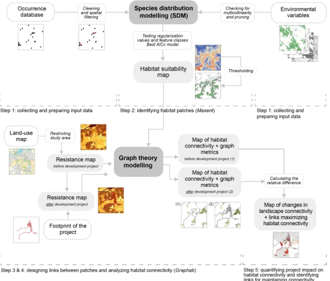
The methodological steps were as follow : i) collecting and preparing input data, i.e. species occurrence datasets and environmental variables; ii) identifying habitat patches based on species distribution modelling using Maxent; iii) designing links between patches using species-specific resistance surfaces; iv) analyzing habitat connectivity based on connectivity metrics taking into account species dispersal capacity using Graphab; v) quantifying development project impact on habitat connectivity and identifying critical landscape elements for maintaining connectivity (Fig. 1).
Fig. 1. Methodological framework applied to evaluate potential change in each species’ habitat connectivity after development project.
2.2. Study site and species occurrence datasets
The study area is located in the suburbs of Lyon, France. It encompasses 1,240 km² of urban (32%), natural habitat (29%) and agricultural (39%) land use (see Section 2.3 for land cover used). The urban and suburban landscapes have been modified since 2012 by a 161-ha project for a new stadium and its
5
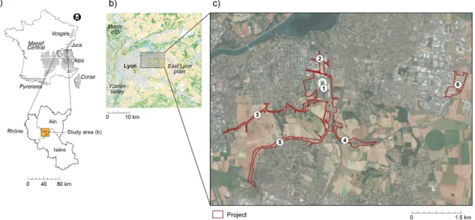
associated developments: extension of a tramway line, creation of an interchange with a national road, construction of public transport lanes, redevelopment of an existing street and creation of a car park (Fig. 2). The major objective of this development project was to fill the gap of Lyon in terms of major sports equipment of regional or national influence in order to answer the European ambitions of the city and county of Lyon.
Fig. 2. Location of the new stadium and its associated developments (1: OL Land Stadium, 2: Extension of the T3 tramway line, 3: Development of existing street, 4: Creation of interchange with national road, 5:
Construction of public transport lanes, 6: Creation of a car park) (c) and location of the project at the regional and national scale (a and b).
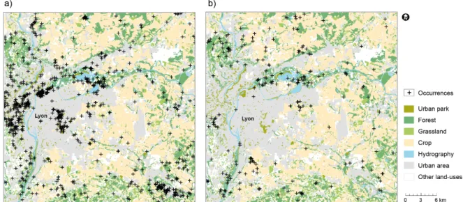
Occurrence data on the red squirrel and the Eurasian badger were obtained from non-governmental organization (NGO) databases created by the League for the Protection of Birds (LPO Ain, Rhône and Isère sections). The surveys feeding the database were conducted by trained observers (naturalist NGOs, managers of natural areas and other partners) between 2000 and 2011 and each observation (by camera trapping or visual observation) was validated by local experts from the LPO. Our database contains 1,299 and 607 records for the red squirrel and the Eurasian badger, respectively (Fig. 3), an appropriate sampling size for the sampling period (11 years).
6
Fig. 3. Land-use map of the study area. Distribution of occurrence points (black cross) for red squirrel (a) and Eurasian badger (b) (from www.faune-ain.org, extracted 18.01.2018, www.faune-rhone.org, extracted 06.11.2017, and www.faune-isere.org, extracted 13.11.2017).
2.3. Environmental data used to identify suitable habitats
Habitat variables and slope (derived from the topography) were extracted from available national databases, i.e. forests, hedges, bushes, moor, heathland, tree plantations, hydrography and transport network are taken from BD TOPO®, topography from RGE ALTI® provided by the French National Geographical Institute (IGN), crop areas and pastures from the French Record of Agricultural Plots (RPG), and urbans areas, sports and leisure facilities, urban and airport from European Urban Atlas provided by the Global Monitoring for Environment Security project. In line with the literature, we selected twelve categories expected to be a priori the most relevant to the habitat preferences (ecological and biological requirements) of the red squirrel (Adren and Delin, 1994; Dylewski et al., 2016; Fey et al., 2016; Hämäläinen et al., 2018; Wauters et al., 2010) and the Eurasian badger (Bouniol, 2017; Dondina et al., 2016; O’Brien et al., 2016). These environmental variables were categorized (Appendix S1) and converted into a 5 m-resolution raster map (Fig. 2c; Fig. 3a) using ArcGIS 10 (Environmental Systems Research Institute, Inc.). For each variable and raster generated, a value was attributed to each cell corresponding to the closest distance between the centroid of the cell and the nearest patch of the habitat variable. We identified collinearity and estimated the importance of the effect of multicollinearity among explanatory variables. We used a stepwise approach to calculate variance inflation factor for each variable (details in Appendix S2).
7
2.4. Step 1: Identifying habitat patches based on species distribution modelling
A maximum entropy modelling approach was implemented, on a large scale (1,240 km²; Fig. 3), to predict species habitat suitability using Maxent, version 3.4.1, to looks for the combination of environmental variables that best explains the distribution of species occurrences (Elith et al., 2011; Phillips et al., 2006). This method is little sensitive to sample size and can generate species response curves to environmental factors (Pearson et al., 2007).
Collaborative databases such as LPO contain observations from different sources or made near urban areas and roads. This sampling bias, called “road-map effect” (Crisp et al., 2001), weakens model performance and results (Beck et al., 2014; Kramer-Schadt et al., 2013). To prevent geographical sampling bias, we therefore implemented a bias file with the package dismo (Hijmans et al., 2017; Team, 2017), calculating a kernel density estimate of sampling effort across the study area. To avoid issues with spatial autocorrelation (i.e. observations recorded at different times from the same location), some occurrence data were removed via spatial filtering, i.e. a procedure for removing spatially clustered points using the SDMtoolbox (Brown et al., 2017). The rarefying distances were selected according to each species’ expected occurrence within this study area: 1.5 to 2 red squirrel individuals per hectare to obtain a mean density of individuals consistent with an urban and suburban context (Chapuis and Marnet, 2006; Rézouki et al., 2014) and 2 Eurasian badger individuals per km², given that Eurasian badger density can range from 4 individuals per km² in favorable environments (i.e. Monts d'Or and Yzeron Valley) to less than 1 in the East Lyon plain (Fig. 2b) (Bouniol, 2017; Malèvre, 2017).
In Maxent, choice of the feature classes can impact types and shapes of the response curves. Recent research suggests that species-specific tuning of Maxent models can improve their performance (Morales et al., 2017). Models based on fine-tuned Maxent settings generally discriminate better than those based on default settings (Fan et al., 2018). Here, a series of Maxent models was implemented with a variety of user-defined settings (i.e. feature classes and regularization multipliers), using software package ENMEval (Muscarella et al., 2014). A model prediction was generated for each combination of feature class and regularization multiplier settings (31 feature classes × 10
regularization multipliers = 310 models), and the most parsimonious and optimal model was selected based on the corrected Akaike Information Criterion (AICc) (Galante et al., 2018; Lobo et al., 2008)
from the unpartitioned dataset.
Models were trained on a random selection of 75% of occurrences and then tested on the remaining 25% to determine the predictive performance of the model. For each training partition, 10 replicates were run (bootstrapping) and the results averaged. Other features were set by default, with a maximum of 2,000 iterations. The outputs of each model were mapped using logistic outputs with continuous probabilities ranging from 0 to 1 (Merow et al., 2013). The performances of final models were
8
evaluated using the true skill statistic (TSS) (Allouche et al., 2006), Cohen’s kappa (Monserud and Leemans, 1992) and AUC (Area Under the receiver operating Curve) (Baldwin, 2009) (Appendix S4). The relative contribution of each environmental variable to the model was assessed using a jackknife procedure. This approach excludes one variable at a time when running the model and provides information on the performance of each variable in the model in terms of how important each variable is at explaining the species distribution and how much unique information each variable provides. Finally, habitat patches were derived from the threshold selection method available in Maxent: maximum training sensitivity plus specificity (MaxTSS), which has been shown to produce highly accurate predictions (Jiménez-Valverde and Lobo, 2007; Liu et al., 2013). We used the mean logistic threshold value from the 15 runs. The minimum area of habitat patches is based on species home range as described in the literature corresponding to 0.5 ha (Bouniol, 2017; Wauters et al., 1994).
2.5. Step 2: Connectivity analysis and assessment of node and link importance
A graph theory approach was used to evaluate habitat connectivity (Foltête et al., 2012b; Pascual-Hortal and Saura, 2006). Links between patches were generated with Graphab software version 2.2 (Foltête et al., 2012a) (http://thema.univ-fcomte.fr/productions/graphab/), using a least-cost path (LCP) based on landscape matrix permeability (Dale and Fortin, 2010; Etherington and Holland, 2013; Rayfield et al., 2010). The least-cost path is the path of least resistance between two patches from the edge of one patch to the nearest edge of another patch through the matrix (Zeller et al., 2012). It represents the shortest functional connection between habitat patches (Adriaensen et al., 2003), which produces the most accurate connectivity estimates (Simpkins et al., 2018). Six resistance values were attributed to the different landscape classes depending on the ability of the species to cross into and survive within them, regardless of habitat suitability (Appendix S3): favorable, suitable, neutral, unfavorable, highly unfavorable or barrier to animal movement. Values ranged from 1 (very low resistance, i.e. habitat patches from Maxent output and other landscape elements) to 10,000 (barrier), with four intermediate classes (50, 100, 400 and 800).
A land-use map was converted into a 5 m-resolution raster map to consider hedges, streams or paths. This map of the initial situation provided a baseline for assessing the impact on habitat connectivity. For the purposes of computing the connectivity index and selecting the most likely inter-patch connections, habitat connectivity took into account a maximum cumulative dispersal distance (cost distance) related to mid- and long-term metapopulation dynamics and gene flow. A threshold of 5,000 m and 2,000 m was chosen for the red squirrel (Avon et al., 2014; Wauters et al., 2010) and the Eurasian badger (Delahay et al., 2000; Do Linh San, 2002; Macdonald and Barrett, 2005),
respectively. The thresholded links showed which patches were currently connected (i.e. formed a network “component”). We converted the Euclidean maximum dispersal distance to cost-distance: a linear regression was performed with Graphab between the values of distances from all the links of
9
the graph. The distances of 5,000 m for the red squirrel and 2,000 m for the Eurasian badger were converted into 32,061 and 6,644 cost units, respectively.
Rao et al. (2018) recommended that a reasonable scale should be considered when measuring the influence of development projects on habitat connectivity. Here, unlike the scale used for Maxent (1,240 km²), we restricted our connectivity analysis according to the spatial configuration of the landscape graph and to the dispersal capacity of the focal species (Huang et al., 2018), i.e. to 6 km either side of the development project (144 km²), a scale that is beyond the maximum dispersal distance of both studied species (2 km and 5 km).
Habitat connectivity was calculated using the Probability of Connectivity index (PC; Eq. 1) proposed by Saura and Pascual-Hortal (2007), a combined measure of habitat amount and connectivity. PC is defined as ‘the probability that two animals randomly placed within the landscape fall into habitat areas that are reachable from each other’, varies between 0 and 1 and is defined as follows.
(1) 𝑃𝐶 = 1 𝐴*+ , -./ + , 0./ 𝑎-𝑎0𝑝-0∗
where n is the total number of patches, and ai and aj are attributes of nodes i and j. Here, the attribute
of the node corresponds to patch area and A represents the total landscape area. The product
probability of a path (where a path is made up of a set of steps in which no patch is visited more than once) is the product of all the pij belonging to each step in that path. pij* is defined as the maximum
product probability of all possible paths between patches i and j (including single-step paths). If patches i and j are close enough, the maximum probability path will be simply the step (direct movement) between patches i and j (pij* = pij). If patches i and j are more distant, the “best”
(maximum probability) path would probably comprise several steps through intermediate stepping stone patches yielding pij* > pij (Saura and Pascual-Hortal, 2007). Here, the probability of connection
between two patches was based on the least-cost distance between these two patches.
Least-cost distance corresponds to the accumulated cost along the least-cost path and was transformed into probability of connection between patches i and j using a decreasing exponential function as shown in Eq. 2.
(2) 𝑝-0= 𝑒6∝89:
where α is a cost distance-decay coefficient: α is usually set so that pij=0.5 for the median or mean
dispersal distance of the focal species, or pij =0.05 for the maximal distance dispersal (Saura and
Pascual-Hortal, 2007), as here.
To indicate the local contribution of each patch to the global PC index, we used the local metric of interaction flux IF (Eq. 3) (Sahraoui et al., 2017).
10 (3) 𝐼𝐹- = + 𝑎-𝑎0
, 0./
𝑒6>89:
The links were ranked according to their contribution to overall habitat connectivity, following the link removal method described in (Saura and Rubio, 2010).
2.6. Step 3: Impact of development project on habitat connectivity
Habitat connectivity for the two species was assessed on the smaller scale (144 km²) before and after the development project to model where ecological connectivity may be lost or reduced (Farrell et al., 2018). A resistance cost of 800 (highly unfavorable to animal movement but not a barrier) was applied to the area concerned by the project (161 ha, termed the “footprint” of the project). The development project impact on habitat connectivity ΔXp was defined as the relative difference in graph metrics
before and after the development project (Eq. 4): (4) 𝛥𝑋B =
𝑋CB− 𝑋EB
𝑋EB × 100
where Xbp and Xap are the landscape metrics before and after the development project, respectively.
Several landscape graph metrics were calculated to describe habitat network characteristics: number and mean size of graph components (ha), number and mean size of habitat patches (ha) and overall and local habitat connectivity (PC and IF).
2.7. Step 4: Identification of links to reconnect in priority
We determined which links, potentially disconnected by the development project, should be
reconnected in priority, i.e. which one could improve global connectivity the most if restored (Foltête et al., 2014). It is possible to make a systematic search using the gtest command in Graphab. This stepwise procedure allows the user to more precisely identify conservation issues from existing habitats patches non-affected by the development project (Fig. 6). The procedure removed from the graph the concerned links (in red on Fig. 5b, d) and then iteratively added the links that maximize the
11
3. Results
3.1. Species distribution modelling
Models for both species fitted the data well, with AUCs > 0.80, TSS > 0.66 and Cohen’s Kappa max > 0.69 (Table 1). Several environmental variables contributed to explaining the distribution of the species in the study area (>3% of total contribution; Table 1). For both species, forest areas showed the greatest contribution to habitat suitability models (59.6% for the red squirrel and 36.5% for the Eurasian badger), followed by crop areas, hedges and bushes and discontinuous urban fabric for the red squirrel, and by discontinuous urban fabric, slope and tree plantations for the Eurasian badger. Jackknife tests on the variables yielded the same results (Appendix S5).
Based on the habitat suitability map, we identified 1,024 and 1,122 habitat patches for the red squirrel and the Eurasian badger, respectively (Appendix S6). Total area of suitable habitats amounted to approximately 262 km² for the red squirrel and 199 km² for the Eurasian badger.
Table 1
Model statistics and relative contribution of environmental variables (>3% of total contribution) to explaining species distribution of the red squirrel and the Eurasian badger in the study area. The table shows mean values (± SD) of the 15 replicates.
Red squirrel Eurasian badger
M od el st at ist ic s AUC training 0.801 ± 0.012 0.883 ± 0.012 AUC test 0.800 ± 0.014 0.800 ± 0.038 TSS 0.701 ± 0.026 0.662 ± 0.036 Kappa max 0.704 ± 0.019 0.687 ± 0.028 R el at iv e con tr ib ut ion o f en vi ron ne m en tal va ri ab le s Forest areas 59.6% 36.5% Crop areas 12.4% 5.2%
Discontinuous urban fabric 4.8% 9.8%
Main transport network 3.7% 6.0%
Slope 7.7%
Tree plantations 6.4%
Densely built-up urban areas 5.7%
Hydrography 5.1%
Hedges and bushes 5.0%
Urban parks 5.0%
Pasture 4.2%
Moors and heathlands 6.3%
3.2. Habitat connectivity analysis
Landscape graphs were based on 157 links for the red squirrel (Fig. 5a) and 106 links for the European badger (Fig. 5b), grouped in 5 and 9 separate components, respectively.
12
The overall connectivity PC was 2.89×10⁻³ for the red squirrel and 1.66×10⁻³ for the Eurasian badger
(Table 2). The local metric of interaction flux IF indicated that many patches significantly contributed to the connectivity of the initial network. The habitat patches with a high contribution were nodes with a large patch size (the criterion considered as a proxy for demographic potential) and/or with a central position that linked them to several other patches in the network.
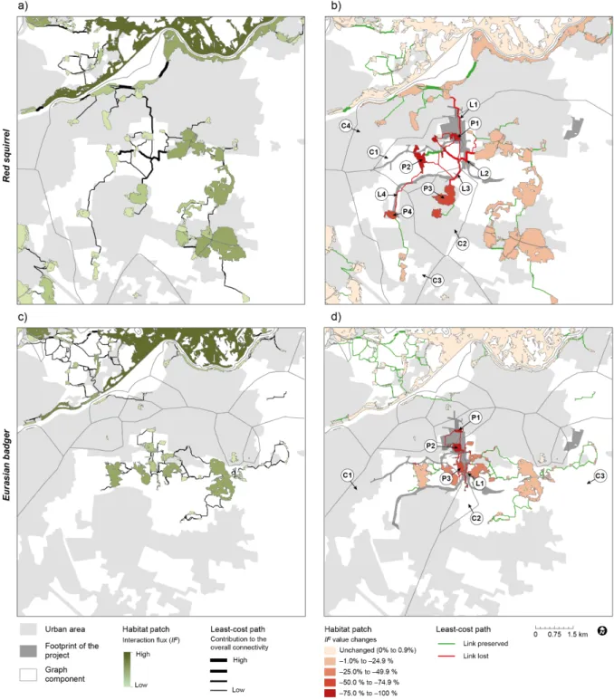
Fig. 5. Landscape graph of the immediate project area (144 km²) showing 1) interaction flux IF of each habitat patch and contribution to the overall connectivity of each link before the development project (a, c), and 2) changes in interaction flux IF of each habitat patch and changes in link structure (link preserved or lost) before and after the development project (b, d) for the red squirrel (a, b) and the Eurasian badger (c, b). Items labeled with the letters correspond to links (Li), habitat patches (Pi) and components (Ci) mentioned in Section 4.
13
3.3. Project impact on habitat connectivity
The development project led to a decrease in PC (–6.8% and –1.8% respectively for the red squirrel and the Eurasian badger) and an increase in the number of graph components (+60.0% and +17.6% respectively) by eliminating links for both species (Table 2; Fig. 5). It removed 12 links for the red squirrel (–7.6%; in red on Fig. 5b) vs. 14 links for the Eurasian badger (–13.2%; in red on Fig. 5d). Some links that strongly contributed to overall habitat connectivity were removed, in particular for the red squirrel (i.e. L1, L2 and L3 in Fig. 5b).
The number of habitat patches decreased by –3.3% (two patches were lost) for the Eurasian badger, while for the red squirrel only mean patch size decreased (–2.0%). The average decrease in IF value for the habitat patches was –11.5% for the red squirrel and –17.7% for the Eurasian badger, with a maximum of –100% where the patch was loss (i.e. P1 and P2 in Fig. 5d). Other habitat patches showed an over 75% decrease in IF value (i.e. P2 in Fig. 5b) or a 50% decrease (i.e. P3 and P4 in Fig. 5b; P3 in Fig. 5d). The maps of the variation in IF for each node (Fig. 5b, d) indicated that the
potential impact was higher when a single component of the graph was divided into several
components (i.e. C1, C2, C3 and C4 in Fig. 5b for the red squirrel, and C1, C2 and C3 in Fig. 5d for the Eurasian badger), or when patch size was substantially reduced (see below).
Table 2. Assessment of the potential impact of the development project on landscape graph metrics, before and after the development project (Xbp and Xap, respectively).
Red squirrel Eurasian badger
Graph characteristics Xbp Xap Variation Xbp Xbp Variation
Number of graph
components 5 8 +60.0% 17 20 +17.6%
Mean size of graph components in ha (min– max) 1,972 (10 – 7,115) 1,644 (10 – 5,355) –16.6% 1,096 (11 – 6,119) 821 (11 – 3,782) –25.1%
Number of habitat patches 80 80 0.0% 60 58 –3.3%
Mean size of habitat patches in ha (min–max) 14.83 (0.52 – 362.28) 14.54 (0.52 – 362,28) –2.0% 10.69 (0.51 – 336.31) 10.61 (0.51 – 336.31) –0.7% Number of links 157 145 –7.6% 106 92 –13.2% PC 2.97×10⁻³ 2.78×10⁻³ –6.8% 1.64×10⁻³ 1.61×10⁻³ –1.8%
3.4. Identification of links to reconnect in priority
The stepwise search for the first 10 links whose reconnection maximizes the PC index yielded Fig. 6, in which the first five links maximizing the most habitat connectivity were identified (Fig. 6a, c). The increase in PC index value following link restoration revealed that the first link restored had a very high contribution to global connectivity gain, and 83.6% of the maximum gain was reached with the
14
10 new links for the red squirrel and 90.1% for the Eurasian badger (Fig. 6b, d). The PC index value did not increase any more after the fifth new link addition, meaning that only the previous links added, and especially the first one, was sufficient to restore global connectivity.
Fig. 6. Location of five links maximizing habitat connectivity for the red squirrel (a) and the Eurasian badger (c). The curves show the gain resulting from the addition of each new link for the red squirrel (b) and the Eurasian badger (d) (see method for details). The dotted line (b, d) corresponds to the initial PC value.
15
We developed a method combining two modelling approaches accessible to environmental consultants and researchers, that would quantify potential loss of the landscape connectivity, so as to provide input to the first part of the mitigation hierarchy in EIA (Bigard et al., 2017). Our results show the
importance of habitat patches and least-cost paths for overall habitat connectivity, crucial to the survival of species. The approach should enable decision-makers to identify key landscape zones where species live or move, like hedges, forests or grasslands, to be preserved in the long term through avoidance and minimization measures. Each step of the methodological framework is discussed below, as well as the limits and possible alternatives of the approach.
4.1. Habitat patch identification and connectivity analysis
The terms “habitat suitability” and “ability to disperse” are often used interchangeably. For instance, Duflot et al. (2018) and Rödder et al. (2016) proposed using SDM-derived maps to calculate a species-specific landscape resistance surface. In this paper, we consider that the movement of species during dispersal is not always subject to the same rules as habitat selection (Keeley et al., 2017; Ziółkowska et al., 2012). Expert-informed resistance maps can thus be an appropriate means of assessing
resistance (Krosby et al., 2015). However, this requires good knowledge of the ecology of the species,
i.e. an expert-based and empirically derived resistance matrix (Reed et al., 2017; Zeller et al., 2012).
Here, this condition was satisfied since the red squirrel and the Eurasian badger are both well-documented species.
The Maxent-derived habitat patches and least-cost paths were presented to a group of experts from local NGOs to obtain an external opinion different from that of local stakeholders. They confirmed our findings based on their knowledge of the study area and the species. However, the goal here was not to qualitatively validate the model outputs. Expert knowledge can usefully be included, for example, to improve species range predictions (Merow et al., 2017), or to qualitatively validate the output maps and response curves from several SDMs (Le Roux et al., 2017). But expert input also has limitations, introducing subjectivity that reduces method reproducibility (Rayfield et al., 2010). Looking at the occurrences only outside habitat patches for the red squirrel, it can be seen that 23.4% of occurrences were recorded less than 20 m from modelled LCPs (least-cost paths), with 75.1% less than 200 m away. For the Eurasian badger, the same pattern was observed, with 16.7% and 83.3% of recorded occurrences respectively. Thus, the LCPs did not exactly represent where the species is likely to move through the landscape. Kool et al. (2013) and Simpkins et al. (2018) suggested testing models with empirical field data, but this analysis shows that it is not easy to observe the corresponding paths in the field. This is because the LCP is only one of many possible paths (actually the shortest one), unlike least-cost corridors (LCC), which represent all viable paths (Avon and Bergès, 2016). Identifying LCPs and LCCs is easier in an area containing a great diversity of land uses that are more or less suitable to species movement (i.e. with higher spatial variation of ecological conditions). In our study
16
area, the high percentage of agricultural land could complicate our analysis, but the density of hedgerows strongly influenced the design of LCPs.
4.2. Estimation of development project impact on habitat connectivity and links to reconnect in priority to implement mitigation or attenuation strategies
The impact assessment method was based on the interaction flux (IF) for habitat patches and on the contribution to the PC for links (Fig. 5a, c). The results show that the spatial extent of the development project leaves many habitat patches isolated in the western part of the red squirrel’s habitat network. The links between the northern and eastern areas were lost (respectively L1 and L2 in Fig. 5b). The loss of L1 may be explained by the removal of a stepping stone habitat (P1 in Fig. 5b) crucial to the movement of species. Other southward links (L2, L3 and L4 in Fig. 5b) were also lost because of the construction of public transport lanes and the interchange with the national road, which represent a barrier for the species. For the Eurasian badger, the only area where animals can disperse was lost (L1 in Fig. 5d), isolating several habitat patches in the western part of the eastern sector (C1 and C2 in Fig. 5d). These changes may affect landscape structure and have a direct impact on the functional habitat connectivity that is vital to the survival of these two terrestrial mammals. On the other hand, the construction of a car park in the eastern sector did not affect habitat connectivity for either species. Our results highlight the conservation challenges related to habitat fragmentation and isolation. Planners and designers' reflections must consider which links to reconnect in priority (Fig. 6) to prioritize and localize restoration efforts. The impacts revealed on habitat patches and links could be used to preserve ecological connectivity at the project scale (Duflot et al., 2018) defining mitigation (and, possibly, also adaptation) strategies at finer scale. To decrease the intensity of the potential impact, the development project must integrate landscape elements favoring the movement of sensitive species among habitat patches (Dalang and Hersperger, 2012). This may involve creating small developments explicitly linking two existing patches, i.e. hedgerows, underground or overhead wildlife crossing structures (respectively, for the Eurasian badger and the red squirrel) between two patches (De Montis et al., 2018; Dondina et al., 2016), or scattered elements (hedgerows or small wooded patches) which modify matrix permeability and act as stepping stones (Ernst, 2014). However, even if all links maximizing the PC index are restored, the initial PC value could not be reached since the total habitat area may have decreased, which was the case for the Eurasian badger (Fig. 6d).
17
4.4. Limitations and alternatives to the methodological framework
To identify habitat patches with Maxent, the main limitation of the proposed methodology is that it requires a set of species occurrence data covering large areas to increase the accuracy and power of species distribution models. Using species records in the process has advantages for interactions between stakeholders, but the exact location of occurrence data is not systematically publicly
available. This can hinder environmental consultants carrying out environmental impact assessments. Using a habitat-oriented approach based on expert opinions or literature is one alternative (Avon and Bergès, 2016; Mimet et al., 2016; Sahraoui et al., 2017). This approach has the advantage of making the ecological network visible and understandable to all the territory's stakeholders. However, this is not species-specific and thus not appropriate for addressing conservation issues involving particularly endangered or emblematic species (Ziółkowska et al., 2012).
Results from a landscape graph can vary significantly depending on data sources, data detail level, knowledge of the ecology of the species, or parameters used. Pereira et al. (2010) recommended testing cost ranges to evaluate the sensitivity of connectivity measures to cost values. However, another recent paper pointed out that connectivity estimates are rather robust to uncertainty in selected cost values, unlike other sources of error, i.e. number of land use represented, spatial resolution or misclassification of edges between landscape classes (Simpkins et al., 2017). Thus, it would be interesting to develop a collaborative database that identifies the elements of the landscape that facilitate species movement (ponds, low walls, wildlife crossings), or breaks in continuity (fences, obstacles) that cannot be detected by photo-interpretation.
Many habitat patches at the study area border had very high IF values (e.g. in the north; Fig. 5a, c), probably because of their attributes (areas). Other small habitat patches located at the border of the study area (i.e. in the west for the Eurasian badger; Fig. 5c) had very little importance for connectivity. However, their importance may be underestimated due to the fact that the land outside the study area was not considered, a well-known problem in spatial analysis (Avon and Bergès, 2016; Gil-Tena et al., 2014). It might be interesting to expand the study area, but caution would be required. Since the PC value depends on the total study area and on the average weight of each habitat patch, increasing the size of the study area could lead to a fairly low PC variation, unless particularly crucial nodes or connections are identified in the full graph.
Finally, other types of relationship between the probability of dispersion and distance between patches
i and j (Eq. 2) could be proposed, for example flat-tailed dispersal kernel, as proposed by some authors
(Nathan et al., 2008) to better account for long-distance dispersal events. Furthermore, note that PC index is only one of the existing methods to calculate habitat connectivity. Topological methods might also be used to evaluate the functional complexity of a landscape (Papadimitriou, 2013). For example,
18
ultrametric distances can help distinguish the relative contribution of each landscape function to the overall complexity of landscape functions in order to create maps of landscape complexity.
5. Conclusion
The development scenario requires finding ways to model ecological processes and functioning (Pereira et al., 2010). Our study shows that combining modelling methods can improve potential environmental impact assessment, providing relevant information for the mitigation process. This is a first step toward applying the method to dimension avoidance and minimization measures. Our methodological framework can also improve the design of the development project to increase its environmental efficiency. A similar step-by-step method can be developed in the design phase to re-evaluate the residual impacts in a meaningful way. This method would re-evaluate the effectiveness of avoidance or mitigation measures in terms of habitat connectivity and resize them if necessary. Finally, if ecological equivalence is not reached at the end of the project design process, our method can also help planners, designers and decision-makers in choosing land where compensation measures can be implemented to reach no net loss of habitat connectivity. In conclusion, our methodology provides a useful tool for EIA studies supporting different land-use planning stakeholders. The insights on habitat connectivity offered by this method, including user-friendly freewares available to all practitioners, will be valuable input to 1) decision-makers and project designers applying the mitigation hierarchy to protect biodiversity and 2) environmental authorities assessing whether development projects will have irreversible effects on the species concerned.
19
Acknowledgements
We thank the LPO (League for the Protection of Birds) for providing species occurrence records. We are grateful to L. Etienne (DAE, Université de Tours) for the GIS improvements and supercomputer facilities that made this project possible. Our thanks to the group of experts, in particular N. Dupire and C. d’Adamo, who showed such interest, support and expertise in species ecology. We thank M. Sweetko for revising the English manuscript, and the ANRT (Association nationale de la recherche et
de la technologie) as well as F. Vullion and F. Theuriau (Soberco Environnement), who contributed to
1
References
Adren, H., Delin, A., 1994. Habitat selection in the eurasian red squirrel, sciurus vulgaris, in relation to forest fragmentation. Oikos 70, 43-48.
Adriaensen, F., Chardon, J., De Blust, G., Swinnen, E., Villalba, S., Gulinck, H., Matthysen, E., 2003. The application of ‘least-cost’modelling as a functional landscape model. Landscape Urban Plann. 64, 233-247. Albert, C.H., Chaurand, J., 2018. Comment choisir les espèces pour identifier des réseaux écologiques cohérents entre les niveaux administratifs et les niveaux biologiques ? Sci. Eaux Territ., 26-31.
Allouche, O., Tsoar, A., Kadmon, R., 2006. Assessing the accuracy of species distribution models: prevalence, kappa and the true skill statistic (TSS). J. Appl. Ecol. 43, 1223-1232.
Avon, C., Bergès, L., 2016. Prioritization of habitat patches for landscape connectivity conservation differs between least-cost and resistance distances. Landscape Ecol. 31, 1551-1565.
Avon, C., Bergès, L., Roche, P., 2014. Comment analyser la connectivité écologique des trames vertes? Cas d'étude en région méditerranéenne. Sci. Eaux Territ., 14-19.
Ayram, C.A.C., Mendoza, M.E., Etter, A., Salicrup, D.R.P., 2017. Anthropogenic impact on habitat
connectivity: A multidimensional human footprint index evaluated in a highly biodiverse landscape of Mexico. Ecol. Indicators 72, 895-909.
Baldwin, R.A., 2009. Use of Maximum Entropy Modeling in Wildlife Research. Entropy 11, 854-866. Beck, J., Böller, M., Erhardt, A., Schwanghart, W., 2014. Spatial bias in the GBIF database and its effect on modeling species' geographic distributions. Ecol. Inform. 19, 10-15.
Bergsten, A., Zetterberg, A., 2013. To model the landscape as a network: A practitioner's perspective. Landscape Urban Plann. 119, 35-43.
Bezombes, L., Gaucherand, S., Kerbiriou, C., Reinert, M.-E., Spiegelberger, T., 2017. Ecological Equivalence Assessment Methods: What Trade-Offs between Operationality, Scientific Basis and Comprehensiveness? Environ. Manage. 60, 216-216-230.
Bigard, C., Pioch, S., Thompson, J.D., 2017. The inclusion of biodiversity in environmental impact assessment: Policy-related progress limited by gaps and semantic confusion. J. Environ. Manage. 200, 35-45.
Bosso, L., Smeraldo, S., Rapuzzi, P., Sama, G., Garonna, A.P., Russo, D., 2018. Nature protection areas of Europe are insufficient to preserve the threatened beetle Rosalia alpina (Coleoptera: Cerambycidae): evidence from species distribution models and conservation gap analysis. Ecol. Entomol. 43, 192-203.
Bouniol, J., 2017. Etat des lieux de la population de Blaireau sur les îles de Crépieux-Charmy. FRAPNA Rhône, p. 23.
Brown, J.L., Bennett, J.R., French, C.M., 2017. SDMtoolbox 2.0: the next generation Python-based GIS toolkit for landscape genetic, biogeographic and species distribution model analyses. PeerJ 5, e4095.
CGDD, 2018. Evaluation environnementale. Guide d’aide à la définition des mesures ERC, Cerema ed. Ministère de la Transition énergique et solidaire. Service de l’économie, de l’évaluation et de l’intégration du développement durable (SEEIDD) du Commissariat Général du Développement Durable (CGDD), Paris, p. 134. Chapuis, J.-L., Marnet, J., 2006. Ecureuils d'Europe occidentale : Fiches descriptives. Muséum National
d'Histoire Naturel (MNHN), Paris, France.
Clauzel, C., Girardet, X., Foltête, J.-C., 2013. Impact assessment of a high-speed railway line on species distribution: Application to the European tree frog (Hyla arborea) in Franche-Comté. J. Environ. Manage. 127, 125-134.
Correa Ayram, C.A., Mendoza, M.E., Etter, A., Salicrup, D.R.P., 2016. Habitat connectivity in biodiversity conservation: A review of recent studies and applications. Prog. Phys. Geog. 40, 7-37.
Crisp, M.D., Laffan, S., Linder, H.P., Monro, A., 2001. Endemism in the Australian flora. J. Biogeogr. 28, 183-198.
Dalang, T., Hersperger, A.M., 2012. Trading connectivity improvement for area loss in patch-based biodiversity reserve networks. Biol. Conserv. 148, 116-125.
Dale, M., Fortin, M.-J., 2010. From graphs to spatial graphs. Annu. Rev. Ecol. Evol. S. 41.
De Montis, A., Ledda, A., Ortega, E., Martín, B., Serra, V., 2018. Landscape planning and defragmentation measures: an assessment of costs and critical issues. Land Use Policy 72, 313-324.
Delahay, R., Brown, J., Mallinson, P., Spyvee, P., Handoll, D., Rogers, L., Cheeseman, C., 2000. The use of marked bait in studies of the territorial organization of the European badger (Meles meles). Mamm. Rev. 30, 73-87.
Do Linh San, E., 2002. Socialité, territorialité et dispersion chez le blaireau européen (Meles meles): état des connaissances, hypothèses et besoins de recherche, L’Etude et la conservation des carnivores. Société Française pour l’Etude et la Protection des Mammifères Paris, pp. 74-86.
Dondina, O., Kataoka, L., Orioli, V., Bani, L., 2016. How to manage hedgerows as effective ecological corridors for mammals: A two-species approach. Agric., Ecosyst. Environ. 231, 283-290.
2
Duflot, R., Avon, C., Roche, P., Bergès, L., 2018. Combining habitat suitability models and spatial graphs for more effective landscape conservation planning: An applied methodological framework and a species case study. J. Nat. Conserv.
Dylewski, Ł., Przyborowski, T., Myczko, Ł., 2016. Winter habitat choice by foraging the red squirrel (Sciurus vulgaris), Ann. Zool. Fenn. BioOne, pp. 194-200.
Ecosphère, 2017. Définition d’une stratégie et d’un plan d’actions de préservation et de restauration de la trame verte et bleue sur le territoire métropolitain. Grand Lyon.
Elith, J., Graham, C.H., Anderson, R.P., Dudik, M., Ferrier, S., Guisan, A., Hijmans, R.J., Huettmann, F., Leathwick, J.R., Lehmann, A., Li, J., Lohmann, L.G., Loiselle, B.A., Manion, G., Moritz, C., Nakamura, M., Nakazawa, Y., Overton, J.M., Peterson, A.T., Phillips, S.J., Richardson, K., Scachetti-Pereira, R., Schapire, R.E., Soberon, J., Williams, S., Wisz, M.S., Zimmermann, N.E., 2006. Novel methods improve prediction of species' distributions from occurrence data. Ecography 29, 129-151.
Elith, J., Phillips, S.J., Hastie, T., Dudík, M., Chee, Y.E., Yates, C.J., 2011. A statistical explanation of MaxEnt for ecologists. Divers. Distrib. 17, 43-57.
Ernst, B.W., 2014. Quantifying landscape connectivity through the use of connectivity response curves. Landscape Ecol. 29, 963-978.
Etherington, T.R., Holland, E.P., 2013. Least-cost path length versus accumulated-cost as connectivity measures. Landscape Ecol. 28, 1223-1229.
Fan, J., Zhao, N., Li, M., Gao, W., Wang, M., Zhu, G., 2018. What are the best predictors for invasive potential of weeds? Transferability evaluations of model predictions based on diverse environmental data sets for Flaveria bidentis. Weed Res. 58, 141-149.
Farrell, L.E., Levy, D.M., Donovan, T., Mickey, R., Howard, A., Vashon, J., Freeman, M., Royar, K., Kilpatrick, C.W., 2018. Landscape connectivity for bobcat (Lynx rufus) and lynx (Lynx canadensis) in the Northeastern United States. PloS one 13, e0194243.
Fey, K., Hämäläinen, S., Selonen, V., 2016. Roads are no barrier for dispersing red squirrels in an urban environment. Behav. Ecol. 27, 741-747.
Foltête, J.-C., Clauzel, C., Vuidel, G., 2012a. A software tool dedicated to the modelling of landscape networks. Environ. Model. Software 38, 316-327.
Foltête, J.-C., Clauzel, C., Vuidel, G., Tournant, P., 2012b. Integrating graph-based connectivity metrics into species distribution models. Landscape Ecol. 27, 557-569.
Foltête, J.-C., Girardet, X., Clauzel, C., 2014. A methodological framework for the use of landscape graphs in land-use planning. Landscape Urban Plann. 124, 140-150.
Galante, P.J., Alade, B., Muscarella, R., Jansa, S.A., Goodman, S.M., Anderson, R.P., 2018. The challenge of modeling niches and distributions for data-poor species: a comprehensive approach to model complexity. Ecography 41, 726-736.
Gil-Tena, A., Nabucet, J., Mony, C., Abadie, J., Saura, S., Butet, A., Burel, F., Ernoult, A., 2014. Woodland bird response to landscape connectivity in an agriculture-dominated landscape: a functional community approach. Community Ecol. 15, 256-268.
Guillera-Arroita, G., Lahoz-Monfort, J.J., Elith, J., Gordon, A., Kujala, H., Lentini, P.E., McCarthy, M.A., Tingley, R., Wintle, B.A., 2015. Is my species distribution model fit for purpose? Matching data and models to applications. Global Ecol. Biogeogr. 24, 276-292.
Hämäläinen, S., Fey, K., Selonen, V., 2018. Research paper: Habitat and nest use during natal dispersal of the urban red squirrel (Sciurus vulgaris). Landscape Urban Plann. 169, 269-269-275.
Herrera, J.M., Alagador, D., Salgueiro, P., Mira, A., 2018. A distribution-oriented approach to support landscape connectivity for ecologically distinct bird species. PloS one 13, e0194848.
Hijmans, R.J., Phillips, S., Leathwick, J., Elith, J., Hijmans, M.R.J., 2017. Package ‘dismo’. Circles 9.
Hofman, M.P., Hayward, M.W., Kelly, M.J., Balkenhol, N., 2018. Enhancing conservation network design with graph-theory and a measure of protected area effectiveness: Refining wildlife corridors in Belize, Central America. Landscape Urban Plann. 178, 51-59.
Huang, J., He, J., Liu, D., Li, C., Qian, J., 2018. An ex-post evaluation approach to assess the impacts of accomplished urban structure shift on landscape connectivity. Sci. Total Environ. 622, 1143-1152.
Jiménez-Valverde, A., Lobo, J.M., 2007. Threshold criteria for conversion of probability of species presence to either–or presence–absence. Acta Oecol. 31, 361-369.
Keeley, A.T., Beier, P., Keeley, B.W., Fagan, M.E., 2017. Habitat suitability is a poor proxy for landscape connectivity during dispersal and mating movements. Landscape Urban Plann. 161, 90-102.
Kiesecker, J.M., Copeland, H., Pocewicz, A., McKenney, B., 2010. Development by design: blending landscape-level planning with the mitigation hierarchy. Front. Ecol. Environ. 8, 261-266.
Kool, J.T., Moilanen, A., Treml, E.A., 2013. Population connectivity: recent advances and new perspectives. Landscape Ecol. 28, 165-185.
3
Kramer-Schadt, S., Niedballa, J., Pilgrim, J.D., Schröder, B., Lindenborn, J., Reinfelder, V., Stillfried, M., Heckmann, I., Scharf, A.K., Augeri, D.M., 2013. The importance of correcting for sampling bias in MaxEnt species distribution models. Divers. Distrib. 19, 1366-1379.
Krosby, M., Breckheimer, I., Pierce, D.J., Singleton, P.H., Hall, S.A., Halupka, K.C., Gaines, W.L., Long, R.A., McRae, B.H., Cosentino, B.L., 2015. Focal species and landscape “naturalness” corridor models offer
complementary approaches for connectivity conservation planning. Landscape Ecol. 30, 2121-2132.
Kujala, H., Whitehead, A.L., Morris, W.K., Wintle, B.A., 2015. Towards strategic offsetting of biodiversity loss using spatial prioritization concepts and tools: A case study on mining impacts in Australia. Biol. Conserv. 192, 513-521.
Le Roux, M., Redon, M., Archaux, F., Long, J., Vincent, S., Luque, S., 2017. Conservation planning with spatially explicit models: a case for horseshoe bats in complex mountain landscapes. Landscape Ecol. 32, 1005-1021.
Liu, C., White, M., Newell, G., 2013. Selecting thresholds for the prediction of species occurrence with presence-only data. J. Biogeogr. 40, 778-789.
Lobo, J.M., Jiménez-Valverde, A., Real, R., 2008. AUC: a misleading measure of the performance of predictive distribution models. Global Ecol. Biogeogr. 17, 145-151.
Lucas, M., 2009. La compensation environnementale, un mécanisme inefficace à améliorer. Revue juridique de l'Environnement, 59-68.
Macdonald, D.W., Barrett, P., 2005. Guide complet des mammifères de France et d'Europe: plus de 200 espèces terrestres et aquatiques. Delachaux & Niestlé.
Malèvre, S., 2017. Etude de la densité d’une population de blaireaux Meles meles en zone périurbaine de la métropole de Lyon, Master Science pour l’Environnement, LBBE Lyon, p. 16.
Merow, C., Smith, M.J., Silander, J.A., 2013. A practical guide to MaxEnt for modeling species' distributions: what it does, and why inputs and settings matter. Ecography 36, 1058-1069.
Merow, C., Wilson, A.M., Jetz, W., 2017. Integrating occurrence data and expert maps for improved species range predictions. Global Ecol. Biogeogr. 26, 243-258.
Mimet, A., Clauzel, C., Foltête, J.-C., 2016. Locating wildlife crossings for multispecies connectivity across linear infrastructures. Landscape Ecol. 31, 1955-1973.
Monserud, R.A., Leemans, R., 1992. Comparing global vegetation maps with the Kappa statistic. Ecol. Model. 62, 275-293.
Morales, N.S., Fernández, I.C., Baca-González, V., 2017. MaxEnt’s parameter configuration and small samples: are we paying attention to recommendations? A systematic review. PeerJ 5, e3093.
Muscarella, R., Galante, P.J., Soley-Guardia, M., Boria, R.A., Kass, J.M., Uriarte, M., Anderson, R.P., 2014. ENMeval: An R package for conducting spatially independent evaluations and estimating optimal model complexity for Maxent ecological niche models. Methods Ecol. Evol. 5, 1198-1205.
Naimi, B., Hamm, N.A., Groen, T.A., Skidmore, A.K., Toxopeus, A.G., 2014. Where is positional uncertainty a problem for species distribution modelling? Ecography 37, 191-203.
Nathan, R., Schurr, F.M., Spiegel, O., Steinitz, O., Trakhtenbrot, A., Tsoar, A., 2008. Mechanisms of long-distance seed dispersal. Trends Ecol. Evol. 23, 638-647.
Newbold, T., Hudson, L.N., Hill, S.L., Contu, S., Lysenko, I., Senior, R.A., Börger, L., Bennett, D.J., Choimes, A., Collen, B., 2015. Global effects of land use on local terrestrial biodiversity. Nature 520, 45.
O’Brien, J., Elliott, S., Hayden, T.J., 2016. Original Investigation: Use of hedgerows as a key element of badger (Meles meles) behaviour in Ireland. Mamm. Biol. 81, 104-104-110.
Papadimitriou, F., 2013. Mathematical modelling of land use and landscape complexity with ultrametric topology. Journal of land use science 8, 234-254.
Pascual-Hortal, L., Saura, S., 2006. Comparison and development of new graph-based landscape connectivity indices: towards the priorization of habitat patches and corridors for conservation. Landscape Ecol. 21, 959-967. Pearson, R.G., Raxworthy, C.J., Nakamura, M., Townsend Peterson, A., 2007. Predicting species distributions from small numbers of occurrence records: a test case using cryptic geckos in Madagascar. J. Biogeogr. 34, 102-117.
Pereira, H.M., Leadley, P.W., Proença, V., Alkemade, R., Scharlemann, J.P., Fernandez-Manjarrés, J.F., Araújo, M.B., Balvanera, P., Biggs, R., Cheung, W.W., 2010. Scenarios for global biodiversity in the 21st century. Science, 1196624.
Phillips, S.J., Anderson, R.P., Schapire, R.E., 2006. Maximum entropy modeling of species geographic distributions. Ecol. Model. 190, 231-259.
Quétier, F., Lavorel, S., 2011. Assessing ecological equivalence in biodiversity offset schemes: key issues and solutions. Biol. Conserv. 144, 2991-2999.
Quétier, F., Regnery, B., Levrel, H., 2014. No net loss of biodiversity or paper offsets? A critical review of the French no net loss policy. Environ. Sci. Policy 38, 120-120-131.
4
Rao, Y., Zhang, J., Xu, Q., Wang, S., 2018. Sustainability assessment of road networks: A new perspective based on service ability and landscape connectivity. Sustain. Cities Soc. 40, 471-483.
Rayfield, B., Fortin, M.-J., Fall, A., 2010. The sensitivity of least-cost habitat graphs to relative cost surface values. Landscape Ecol. 25, 519-532.
Reed, G., Litvaitis, J., Callahan, C., Carroll, R., Litvaitis, M., Broman, D., 2017. Modeling landscape
connectivity for bobcats using expert-opinion and empirically derived models: how well do they work? Anim. Conserv. 20, 308-320.
Rézouki, C., Dozières, A., Le Cœur, C., Thibault, S., Pisanu, B., Chapuis, J.-L., Baudry, E., 2014. A Viable Population of the European Red Squirrel in an Urban Park. PLoS ONE 9, 1-1-7.
Rödder, D., Nekum, S., Cord, A.F., Engler, J.O., 2016. Coupling satellite data with species distribution and connectivity models as a tool for environmental management and planning in matrix-sensitive species. Environ. Manage. 58, 130-143.
Sahley, C., Vildoso, B., Casaretto, C., Taborga, P., Ledesma, K., Linares-Palomino, R., Mamani, G., Dallmeier, F., Alonso, A., 2017. Quantifying impact reduction due to avoidance, minimization and restoration for a natural gas pipeline in the Peruvian Andes. Environ. Impact Assess. Rev. 66, 53-65.
Sahraoui, Y., Foltête, J.-C., Clauzel, C., 2017. A multi-species approach for assessing the impact of land-cover changes on landscape connectivity. Landscape Ecol. 32, 1819-1835.
Saura, S., Pascual-Hortal, L., 2007. A new habitat availability index to integrate connectivity in landscape conservation planning: comparison with existing indices and application to a case study. Landscape Urban Plann. 83, 91-103.
Saura, S., Rubio, L., 2010. A common currency for the different ways in which patches and links can contribute to habitat availability and connectivity in the landscape. Ecography 33, 523-537.
Scolozzi, R., Geneletti, D., 2012. A multi-scale qualitative approach to assess the impact of urbanization on natural habitats and their connectivity. Environ. Impact Assess. Rev. 36, 9-22.
Simpkins, C.E., Dennis, T.E., Etherington, T.R., Perry, G.L., 2017. Effects of uncertain cost-surface specification on landscape connectivity measures. Ecol. Inform. 38, 1-11.
Simpkins, C.E., Dennis, T.E., Etherington, T.R., Perry, G.L., 2018. Assessing the performance of common landscape connectivity metrics using a virtual ecologist approach. Ecol. Model. 367, 13-23.
Tannier, C., Bourgeois, M., Houot, H., Foltête, J.-C., 2016. Impact of urban developments on the functional connectivity of forested habitats: a joint contribution of advanced urban models and landscape graphs. Land Use Policy 52, 76-91.
Team, R.C., 2017. R: A language and environment for statistical computing. Vienna, Austria: R Foundation for Statistical Computing; 2016.
Wauters, L., Casale, P., Dhondt, A.A., 1994. Space use and dispersal of red squirrels in fragmented habitats. Oikos, 140-146.
Wauters, L.A., Verbeylen, G., Preatoni, D., Martinoli, A., Matthysen, E., 2010. Dispersal and habitat cuing of Eurasian red squirrels in fragmented habitats. Popul. Ecol. 52, 527-536.
Zeller, K.A., McGarigal, K., Whiteley, A.R., 2012. Estimating landscape resistance to movement: a review. Landscape Ecol. 27, 777-797.
Ziółkowska, E., Ostapowicz, K., Kuemmerle, T., Perzanowski, K., Radeloff, V.C., Kozak, J., 2012. Potential habitat connectivity of European bison (Bison bonasus) in the Carpathians. Biol. Conserv. 146, 188-196.