Analysis of inefficiencies in shipment data handling

Analysis of Inefficiencies in Shipment Data Handling

by

Rohini Prasad

Master of Business Administration, Indian School of Business, 2014

Bachelor of Engineering, Information Technology, University of Pune, 2010

and

Gerta Malaj

Bachelor of Arts, Mathematics, Wellesley College, 2013

SUBMITTED TO THE PROGRAM IN SUPPLY CHAIN MANAGEMENT

IN PARTIAL FULFILLMENT OF THE REQUIREMENTS FOR THE DEGREE OF

MASTER OF ENGINEERING IN SUPPLY CHAIN MANAGEMENT AT THE

MASSACHUSETTS INSTITUTE OF TECHNOLOGY

JUNE 2017

Q

2017 Rohini Prasad and Gerta Malaj. All rights reserved.

The authors hereby grant to MIT permission to reproduce and to distribute publicly paper and

electronic copies of this thesis document in whole or in part in any medium now known or

hereafter created.

k

Signature redacted

Signature of A utho r...

...

Master of Engineer'i' in Supply Chain Management

Signature of Author...Signature

redacted

M t

Vof F

gineerfh in Supply Chain Management

Signature redacted

12,

C e rtifie d b y

...

...

Dr. Matthias Winkenbach

Director, MIT Megacity Logistics Lab

Thesis Supervisor

Signature redacted

A cce p te d b y

...

V

ARCHIVES

Director, Center for Transportation and Logistics

MASSACHUSETTS INSTITUTE

Elisha Gray

11

Professor of Engineering Systems

Analysis of Inefficiencies in Shipment Data Handling

by

Rohini Prasad

and

Gerta Malaj

Submitted to the Program in Supply Chain Management

on May 12, 2017 in Partial Fulfillment of the

Requirements for the Degree of Master of Engineering in Supply Chain Management

ABSTRACT

Supply chain visibility is critical for businesses to manage their operational risks. Availability of

high quality and timely data regarding shipments is a precursor for supply chain visibility. This

thesis analyses the errors that occur in shipment data for a freight forwarder. In this study, two

types of errors are analyzed: system errors, arising from violations of business rules defined in

the software system, and operational errors, which violate business rules or requirements

defined outside the software. We consolidated multifarious shipment data from multiple sources

and identified the relationship between errors and the shipment attributes such as source or

destination country. Data errors can be costly, both from a human rework perspective as well as

from the perspective of increased risk due to supply chain visibility loss. Therefore, the results of

this thesis will enable companies to focus their efforts and resources on the most promising error

avoidance initiatives for shipment data entry and tracking. We use several descriptive analytical

techniques, ranging from basic data exploration guided by plots and charts to multidimensional

visualizations, to identify the relationship between error occurrences and shipment attributes.

Further, we look at classification models to categorize data entries that have a high error

probability, given certain attributes of a shipment. We employ clustering techniques (K-means

clustering) to group shipments that have similar properties, thereby allowing us to extrapolate

behaviors of erroneous data records to future records. Finally, we develop predictive models

using Naive-Bayes classifiers and Neural Networks to predict the likelihood of errors in a record.

The results of the error analysis in the shipment data are discussed for a freight forwarder. A

similar approach can be employed for supply chains of any organization that engages in physical

movement of goods, in order to manage the quality of the shipment data inputs, thereby

managing their supply chain risks more effectively.

Thesis Supervisor: Dr. Matthias Winkenbach

Title: Director, MIT Megacity Logistics Lab

ACKNOWLEDGEMENTS

We would like to thank everyone who has supported us in completing this thesis. Our special

acknowledgements go to our thesis advisor, Dr. Matthias Winkenbach, for providing us with his

inestimable guidance, insightful discussions, and deep expertise. The magnitude and significance

of Matthias' leadership and constant encouragement to find new ways of exploring and

presenting our thesis content cannot be overstated.

We would also like to express our gratitude to our sponsor company, Damco, for giving us their

time, data and invaluable insights on this thesis. Finally, we would like to thank the entire MIT

SCM cohort for their generous contributions to our education; and our families and friends for

their tremendous support.

Table of Contents

ACKNOW LEDGEM ENTS ... 3

L ist o f F ig u re s ... 6

List o f T a b le s...8

Glossary of Terms and Acronyms ... 9

1 . In tro d u ctio n ... 1 1 1.1 Background and Research Question... 11

1.2 Thesis Scope and Structure ... 12

2 . Lite ratu re re v ie w ... 1 3 2.1 Analytics in Supply Chains ... 13

2 .1 .1 D e scriptive A n a lytics ... 1 3 2 .1 .2 P re d ictiv e A n a lytics ... 15

2.1.3 Prescriptive Analytics ... 18

2.2 Analytics techniques for predicting data entry errors ... 20

2.2.1 Phrasal Statistical M achine Translation ... 20

2.2.2 XML (eXtensible M arkup Language) data models ... 21

2 .2 .3 A rtificial intellig e n ce ... 2 2 3 . M e th o d o lo g y ... 2 3 3 .1 G e n e ra l A p p ro a ch ... 2 3 3.2 Data collection and cleaning ... 25

3 .2 .1 D ata so u rce s ... 2 5 3.2.2 Data Preparation ... 27 3.3 M odel Development...30 3 .3 .1 D e scriptive a n a lysis ... 3 0 3 .3 .2 P re d ictive A n a lysis ... 3 1 3 .3 .3 P re scriptive A n a ly sis ... 3 6 3 .4 M o d e l V a lid atio n ... 3 7 4 . C a se Stu dy A n alyisis ... 4 1 4.1 Damco Operational Context ... 41

4 .2 D a ta C o lle ctio n ... 4 2 4 .2 .1 D ata so u rce s ... 4 2 4.2.2 Data Cleansing and Organization ... 44

4 .2 .3 D a ta Ex ce p tio n s ... 4 7

4.3 M odel Development ... 49

4.3.1 Descriptive Analytics ... 49

4.3.2 Predictive Analytics ... 98

4.3.3 Prescriptive analytics ... 109

4.4 Im plications and Discussion ... 110

4 .5 Lim ita tio n s ... 1 1 1 5 . C o n c lu s io n ... 1 1 1 6 . R e fe re n c e s ... 1 1 3

List of Figures

Figure 1: Four-phase analysis m ethodology ... 23

Fig ure 2 : A nalytics M aturity M o del ... 24

Figure 3: Data Tem plate for data consolidation ... 26

Fig u re 4 : Illustrative RO C g rap h ... 38

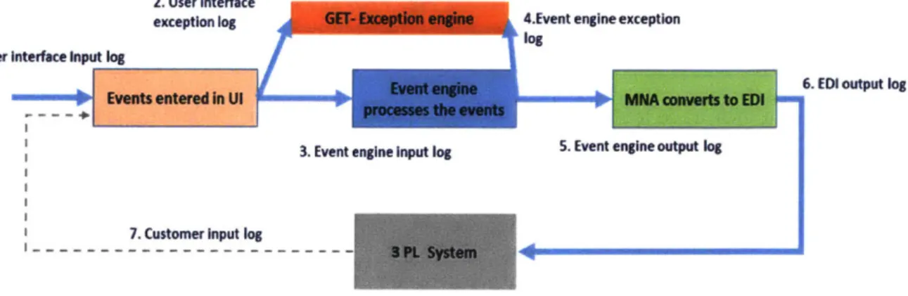
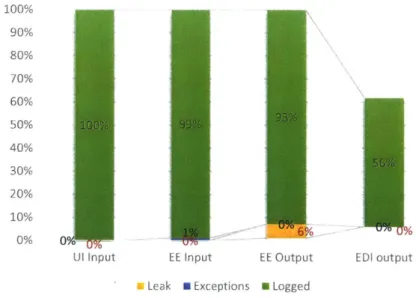
Fig u re 5 : Inte r-syste m D ata Flo w ... 4 2 Figure 6: Data propagation through Dam co system s ... 44

Fig u re 7 : D ata e xce ptio n s ... 4 8 Figure 8: Data Categorization by Status of each record ... 50

Figure 9: Transactions between Origin-Destination pairs ... 51

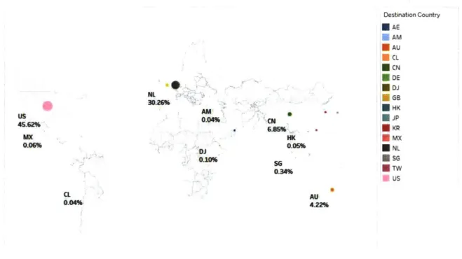
Figure 10: Transaction distribution to Destination countries ... 52

Figure 11: Plot of number of distinct shipments mapped against each event ... 52

Figure 12: Plot of number of records mapped against each event ... 53

Figure 13: Plot of num ber of events tracked for shipment ... 54

Figure 14: Relative occurrences of System errors, by day ... 57

Figure 15: System errors against all entries, by day ... 57

Figure 16: Absolute occurrences of System errors by month ... 58

Figure 17: Relative occurrences of System errors by month ... 58

Figure 18: Absolute System Error distribution by day of week ... 59

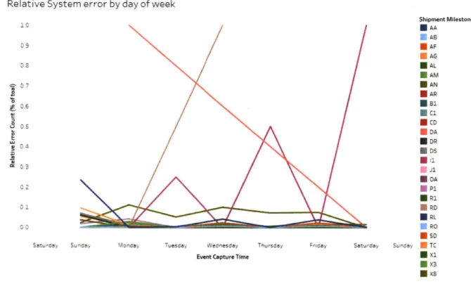
Figure 19: Relative System Error distribution by day of week... 60

Figure 20: Time difference between data corrections/updates(a and b)...61

Figure 21: Histogram of 'Tim eSince First' distribution ... 62

Figure 22: M edian 'Tim eSince Last' by event-code ... 63

Figure 23: M ean 'Tim eSince Last' by event-code ... 63

Figure 24: 'Tim eSinceFirst' distribution by Event-Code... 64

Figure 25: 'Tim eSinceFirst' m ean by Event-Code ... 65

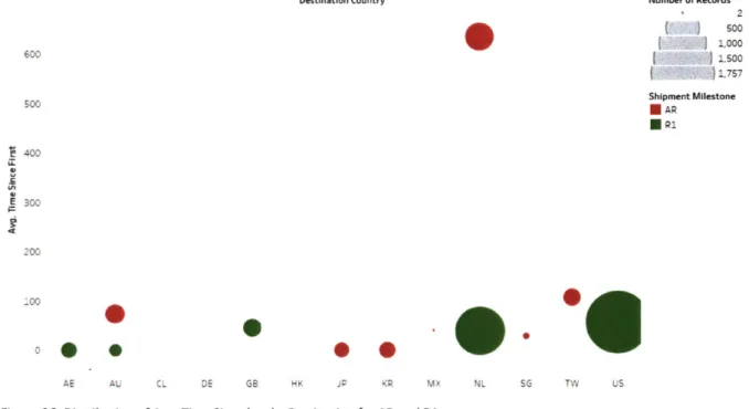
Figure 26: Distribution of Avg. Time Since last by Destination for AR and R1...66

Figure 27: Absolute and relative distribution of corrections by day of week...66

Figure 28: Absolute and relative distribution of corrections by day of month ... 67

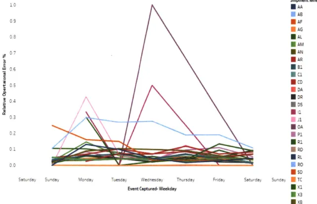
Figure 29: Relative Operational Error distribution by day of week ... 68

Figure 30: Occurrence of Edited Fields and both relative and absolute corrections by quarter ... 69

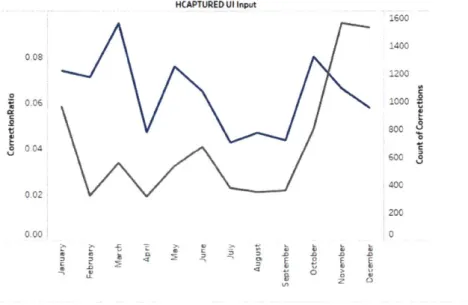
Figure 31: Occurrence of Edited Fields and both relative and absolute corrections by month ... 70

Figure 32: Occurrence of Edited Fields and both relative and absolute corrections by weekday...70

Figure 33: Absolute System Errors by Users... 72

Figure 34: Relative System Errors by Users ... 73

Figure 35: O perational Errors by U sers ... 74

Figure 36: Relative distribution of transactions and shipments by consignee ... 75

Figure 37: Relative distribution of transactions and shipments by consignee, colored by status...76

Figure 38: 'Tim eSinceLast' by destination country (a and b) ... 77

Figure 39: 'Tim eSinceFirst' by destination country (a and b) ... 78

Figure 40: Relative distribution of records by event ratio and destination country...79

Figure 41: Relative distribution of records and shipments by event ratio and destination country ... 80

Figure 43: Correction versus total status for each Edited Field, broken down by Origin Country... 81

Figure 44: Correction versus total status for each Edited Field, broken down by Event Country ... 82

Figure 45: Relative distribution of transactions by event count... 83

Figure 46: Relative distribution of transactions by event count Initial Entries... 84

Figure 47: Relative distribution of transactions by event count Correction ... 84

Figure 48: Relative distribution of transactions by event count - Redundant ... 85

Figure 49: Relative distribution of transactions by event count Update ... 86

Figure 50: Absolute distribution of events per shipment colored by status ... 87

Figure 51: Relative distribution of Shipment by status and event-code... 88

Figure 52: Distinct delayed shipment data by source-destination country ... 89

Figure 53: Reason code data by source-destination country ... 89

Figure 54: Absolute shipment distribution by reason code and status ... 90

Figure 55: Relative shipment distribution by reason code and status ... 91

Fig u re 5 6 : Ed ite d Fie ld s by M o d e ... 9 2 Figure 57: Edited Fields by Status... 92

Figure 58: Edited Fields by Reason Code ... 93

Figure 59: Edited Fields by Event Code ... 93

Figure 60: Edited Fields by Consignee ... 94

Fig u re 6 1 : Scatte rp lo t o f cluste rs ... 9 6 Fig u re 6 2 : K -m e a n s B ip lo t ... 9 6 Fig u re 6 3 : N e u ra l N et 1 M o d e l ... 10 1 Figure 64: Neural Net 1- ROC curve...102

Figure 65: Neural Net 2 Model ... 103

Figure 66: Neural Net 2- ROC curve...104

Figure 67: Neural Net 3 model ... 105

Figure 68: Neural Net 3- ROC curve...106

Figure 69: Neural Net 4 model ... 107

List of Tables

Table 1: Activation Functions for Neural Nets... 36

Table 2: Goodness-of-Fit m etrics ... 39

Table 3: Data Dictionary ... 45

Table 4: Tem poral variation of Edited Fields ... 71

Table 5: K-M eans Clustering CCC... 95

Table 6: Count of records per cluster ... 96

Table 7: Naive Bayes-1 classification result ... 98

Table 8: Naive Bayes-2 classification result ... 99

Table 9: Naive Bayes-3 classification result ... 99

Table 10: Naive Bayes-3 adjusted confusion m atrix... 99

Table 11: Naive Bayes-4 classification result ... 100

Table 12: Naive Bayes-4 adjusted confusion m atrix...100

Table 13: Neural Net 1 Perform ance ... 101

Table 14: Neural Net 1 Confusion M atrix and Rates ... 102

Table 15: Neural Net 2 Perform ance ... 103

Table 16: Neural Net 2 Confusion M atrix and Rates ... 103

Table 17: Neural Net 3 Perform ance ... 105

Table 18: Neural Net 3 Confusion M atrix and Rates (Training) ... 105

Table 19: Neural Net 3 Confusion M atrix and Rates (Validation)...105

Table 20: Neural Net 4 Perform ance ... 107

Table 21: Neural Net 4 Confusion M atrix and Rates (Training) ... 107

Table 22: Neural Net 4 Confusion M atrix and Rates (Validation) ... 107

Glossary of Terms and Acronyms

" ABS - Agent Based Simulation

" AHP - Analytic Hierarchic Process

" ALMIL - Adaptive Language Modeling Intermediate Layer

" ARIMA - Autoregressive Integrated Moving Average

" AUC - Area under the curve, of the ROC plot * CART - Classification and Regression Trees * DES - Discrete-Event Simulation

" EDI - Electronic Data Interchange

" FETA - Forecasted Expected Time of Arrival

" GET - Global Exception Tool, where all the system exceptions funnel through

" MAD - Mean Absolute Deviation " MAE - Mean Average Error

" MAPE - Mean Average Percentage Error " MNA - Messaging and Alerting system

" NLP - Natural Language Processing

" OLAP - Online Analytical Processing " PCA - Principal Component Analysis

" RMSE - Root Mean Square Error

" ROC - Receiver- Output Characteristics, a graph of the model's Sensitivity against (1 - Specificity) " RSS - Really Simple Syndication

" SD - System Dynamics

" SMT - Statistical Machine Translation

" UI - User Interface, the system used by Damco to input all shipment-milestone data

" Waybill - a document issued by a carrier outlining details and instructions about a shipment of goods. Sometimes you can have many events for each waybill, and many waybills per container. However, for our dataset, it is one-to-one. Therefore, waybill and shipment are used analogously.

1. Introduction

1.1 Background and Research Question

Our thesis sponsor, Damco, is a freight forwarding and supply chain management service provider. One key task that they perform is the tracking of each shipment for the customer. They classify the shipment transit lifecycle across multiple milestones, such as 'Dispatch', 'Arrival at port', and 'Awaiting customs clearance'. This thesis focuses on the application of analytics to determine the probability and likely cause of data entry errors while recording the key milestones associated with a shipment. Real-time tracking is essential for supply chain visibility. The majority of Damco's customers track an industry standard list of 8 shipment milestones per shipment. The shipment-milestone data for these customers is updated systemically using Electronic Data Interchange (EDI). However, there are a number of non-standard milestones required by a few customers, which require manual tracking and update, especially for air shipments. These entries have an increased probability of error due to the manual intervention involved, which can result in missing updates or data entry errors. Moreover, as supply chains become more global and complex, visibility becomes both more important and more challenging. The repercussions of data errors can be detrimental for Damco's clients. Any organization involved in the movement of goods faces similar challenges. Our approaches and findings can, therefore, also be effective for these organizations. The customer data analyzed for this review is from one of Damco's non-standard customers who requires tracking of multiple shipment-events in addition to the industry standard set. Although this issue currently reflects a problem with one of Damco's customers, descriptive and predictive analytics can be applied toward all customers in the near future as Damco's machine-intelligence matures, becoming more accurate and potentially prescriptive. This thesis explores some the descriptive and predictive techniques that Damco could utilize in this process.

Although we have analyzed several research papers on the analytical techniques used in supply chain and data error detection, this is a deep and diverse field, and research topics tend to specialize on specific real world problems, such as in weather forecasting, traffic incident forecasting, and natural language error detection and correction. Analysis of the current techniques used in grammatical and lexical corrections gives us useful insights on how to anticipate and remedy human data entry error. By using a hybrid model that utilizes both descriptive and prescriptive analysis, our thesis develops a reusable framework for data entry error detection and correction. This framework will help improve supply chain visibility, particularly for the logistics function, where the cost of missing data and data error is high.

1.2 Thesis Scope and Structure

The rest of this thesis is organized as follows. Section 2 presents a summary of the literature review on the use of analytics in supply chains and the main methods and challenges related to them. In section 3, we present the methodological framework that we developed to identify the root cause of the shipment error and to deduce the probability of errors in future shipment data entries based on the historical trends. We use descriptive analytics techniques for the former and predictive analytics for the latter. Additionally, we apply this framework to a practical example as a case study, which is laid out in section 4. Finally, we discuss the limitations associated with our case study, arising from data unavailability, as well as limitations of the proposed methodological approach.

2. Literature review

This literature review focuses on two key areas: First, the use of analytics in supply chains and the key trends and challenges related to them; Second, the existing techniques used and case studies demonstrating data error detection and correction.

2.1 Analytics in Supply Chains

Data analytics can be broken down into three main categories: descriptive, predictive, and prescriptive analytics. Each of these categories of analysis provides unique insights into the nature and performance of current supply chain processes, as well as the potential properties of future supply chain processes. In this section, we explore some of the work done in each of these three categories of analytics with a focus on supply chain data.

2.1.1 Descriptive Analytics

Statistical analysis is a key part of descriptive analysis. It includes both quantitative and qualitative analysis. Qualitative analysis has limited use and is usually adopted only when there is limited quantitative data available or while analyzing subjective data that requires the judgment of an expert (Wang, Gunasekaran, Ngai, & Papadopoulos, 2016). Statistical analysis may also intersect with the domain of descriptive analytics (such as time series analysis) or predictive analytics (such as regression analysis).

Oliveira, McCormack, & Trkman (2012) make a compelling case for the need for analytics in supply chains, stating that it helps in visualizing supply chain performance not just for the individual players in the supply chain - suppliers, distributors, manufacturers, retailers - but also for the supply chain as a whole. They argue that the primary role of business analytics, particularly descriptive and predictive, is to increase the propensity of information processing and exchange in an organization (Oliveira et al., 2012). To assess the impact of business analytics on different stages of the supply chain, this study uses the supply chain

operations reference (SCOR) framework. SCOR is a management tool for addressing and communicating supply chain management decisions within a company and with its suppliers and customers. The study looks at supply chains as a set of four sequential phases: 'Plan', 'Source', 'Make', and 'Deliver'. The 'Deliver' phase entails the key logistics processes that are a subject of our thesis. The study shows that, except for the case of companies with the most mature supply chains (classified as Level 1), supply chain performance in the 'Deliver' phase is enhanced significantly by the deployment of business analytics (Oliveira et al., 2012).

An example of the decision making process during the SCOR's 'Plan' phase is demand forecasting using descriptive and predictive analytics. Demand forecasting is essential for supply chain planning. Different scenarios may involve different analytics techniques. Causal forecasting methods, used to analyze factors that affect demand for a product, include linear, non-linear, and logistic regression. As an example, consider the relationship between demand forecasting and the production planning process. Parts have dependent demand, as their demand depends on the SKUs that use those parts. Conversely, SKUs themselves have independent demand. While the demand for items that have dependent demand can be derived from the corresponding SKU's demand, forecasting the demand for items that have independent demand involves predictive analytics. This forecasting is generally achieved using time-series methods, for which the only predictor of demand is time.

One of the predictive analytics techniques, autoregressive modeling, involves deriving demand forecasts for any given period as a weighted sum of demands in the previous periods. Autoregressive modeling looks at a value from a time series and regresses it on previous values from that same time series, which are obtained from descriptive analytics (Souza, 2014). Thus, this technique demonstrates how predictive analytics relies on descriptive analytics.

Big data has taken center-stage in conversations on analytics. Per a definition proposed by De Mauro, Greco, & Grimaldi (2015), "Big Data represents the Information assets characterized by such a high volume, velocity and variety to require specific technology and analytical methods for its transformation into value". The availability of big data poses a new set of challenges for supply chains especially when it comes to identifying what is important and to finding the skills needed to derive insights from this data within one's supply chain (Wang et al., 2016). Descriptive analytics gives organizations a better understanding of what happened in the past, when it happened, and what is happening at present. The descriptive techniques referred to by Wang et al. (2016) are either performed at standard periods or as needed using online analytical processing (OLAP) techniques. Other techniques used in studies and practical applications include descriptive statistics such as sums and averages, as well as variants of time series and regression analysis.

2.1.2 Predictive Analytics

Predictive analytics techniques include regression, time series analysis, classification trees, and machine learning techniques such as neural networks. The most common technique used for predictive analysis and forecasting is the use of regression models. The simple linear regression model, the most basic variant of regression models, assumes that the relationship between a dependent variable (y) and an independent variable (x) is approximately linear. The method uses a least squares point estimate to find the slope and intercept of this line (Bowerman, O'Connell, & Koehler, 2005). Simple linear regressions can be extended to include multiple independent variables, giving us the multiple linear regression model. This can be expressed in the form:

Y Where X + 1X1 + #2X2 + --- i+ vapx, + E

Alternatively, a quadratic regression model which uses the equation of a parabola of the form

y = fiO +

fix

f3

to establish the relationship between the dependent and independent variables is also just a variant of the simple regression model since it is a linear combination of parameters (Bowerman et al., 2005).

On the other end of the spectrum, predictive analytics includes advanced mathematical models often supplemented with programming techniques to use historical data to predict a likely future. A key step in predictive analytics is therefore to identify the appropriate explanatory variables from among all the input variables. For instance, in logistics operations, given the proliferation of big data, logistics planning problems - formulated as network flow problems - can be optimized effectively from supply to demand. Due to supply disruptions and demand uncertainty prevalent in supply chains, which directly impacts the logistics operations, predictive models play a critical role in modeling supply chain flexibility into logistics operations. The predictive analytics techniques covered in Wang et al. (2016) refers to the use of mathematical algorithms and programming models to help project what will happen in the future and why.

A key challenge faced is that the analysis of multi-dimensional data is often computationally expensive

(Wang et al., 2016). Dimension reduction is a common precursor before execution of supervised learning methods (Shmueli, Bruce, Stephens, & Patel, 2016). Principal component analysis (PCA) is the most common technique used to address the 'Curse of dimensionality' problem. PCA is a statistical technique for dimensionality reduction. It seeks to capture the maximum amount of information about the data in a low dimensional representation, by performing a linear projection of the original high-dimensional feature vectors (Chang, Nie, Yang, Zhang, & Huang, 2016). These vectors, called the principal components (PCs), are a linear combination of the input variables weighted by so-called factor loadings. Within a multi-dimensional dataset, the first principal component represents the direction in which the variability is the largest. Each subsequent axis has the highest variance, after constraining the preceding principal axis.

However, the results of a PCA, the so-called principal components, are often hard to interpret. To overcome this challenge, a sparse principle component analysis (SPCA) approach can be utilized which is computationally less expensive and more generalizable. One possible approach which is commonly used to reduce dimensionality under SPCA is to manually set factor loadings (which are below a certain threshold) to zero. Another approach is to reformulate the PCA as a regression-type optimization problem and to run an optimization algorithm to calculate the factor loadings, in an attempt to end up with as few predictors as possible. To find the optimal solution efficiently for this optimization problem, the problem must be formulated as a convex function. Niculescu & Persson (2006) define convex functions as having two main properties which make them well suited for optimization problems: (i) the maximum is attained at the boundary; and (ii) any local minimum is a global minimum. The SPCA algorithm, which uses optimization to reduce the number of explicitly used variables, performs well in finding a local optimum but since it is not convex, it is difficult to ensure that it finds the global optimum. To address this problem, Chang et al. (2016) proposed a convex PCA formulated as a low rank optimization problem based on the hypothesis (and its associated proof) that SPCA is equivalent to regression. For a given dataset (represented as a vector), a sparse representation attempts to minimize the number of non-zero entries in the vector. In contrast, a low-rank representation seeks to minimize the rank of the matrix containing the data entries (Oreifej & Shah, 2014). Recall that the rank of a matrix is defined as the maximum number of linearly independent column (or row) vectors in the matrix. For a 'r x c' matrix with 'r' rows and 'c' columns, the maximum rank will be the minimum of r and c. Stat Trek (2017) offers more details on how to compute rank of a matrix.

Unsupervised and supervised learning techniques are other important prediction analysis techniques. Supervised learning techniques are used in classification and prediction. They require the availability of the outcome of interest, which is referred to as the labelled field. For example, in the case of shipment data for a freight forwarder (as shown in section 4. Case Study Analysis), a labeled field can be used to denote

whether the record contains errors (Yes/ No). The data set is segmented into training and validation data. The model learns the relationship between the predictor and outcome variable from the training data. The relationship is then applied to the validation dataset to assess its performance. Classification and prediction most commonly use supervised learning (Shmueli et al., 2016).

Unsupervised learning techniques do not have any pre-specified outcome variable, so, association rules are used as part of the learning algorithm, instead. Within unsupervised learning, clustering is the most commonly used technique (Albalate & Minker, 2013). Some of the popular clustering approaches are hierarchical, partitional, model-based, density-based and graph-based algorithms. An example of partitional and non-hierarchical clustering is k-means. K-means is a method of partitioning 'n' observations into k clusters while each observation belongs to the cluster with the nearest mean. K-means is the most frequently used partitional clustering method, as it is versatile, easy to implement, and, most notably, it does not change with varying data orderings (Celebi et al., 2013).

2.1.3 Prescriptive Analytics

The logical evolution of descriptive and predictive analytics is prescriptive analytics that works by identifying and defining business rules that subsequently trigger a required action when the input condition is met. Schaffhauser (2014) lists 12 key components necessary for successful implementation and use of prescriptive analytics based on an interview with University of Wisconsin-Green Bay's CIO, Rajeev Bukralia. The two most critical questions to be asked are whether the problem lends itself well to prescriptive analysis and how it can be cross-validated for determining predictive accuracy of the model. This can be accomplished by partitioning the data into two datasets - training and validation dataset - before developing the model using the training dataset. The validation dataset can be used to test the efficacy of the model. Defining business rules is another key step for ensuring that the prescriptive output is insightful and the role of the core operations teams in this task cannot be emphasized enough. The knowledge of how the prescriptive system should behave (as captured in the business rules) lies with the people who are

performing the task (which is to be enhanced with prescriptive analysis) on a daily basis. Establishing project management guidelines and data governance mechanisms - including a consistent methodology to determine what data is relevant for prescriptive analysis - is imperative. Finally, Schaffhauser (2014) reminds the reader that prescriptive analytics can fail for new unseen scenarios for which the business rules have not been defined and the model hasn't been trained.

Prescriptive analytics involves looking at historical data, applying mathematical models, and superimposing business rules in order to identify, recommend, or implement alternative decisions (Wang et al., 2016). This is valuable for the comparison of alternative decisions that involve complex objectives and large sets of constraints. Prescriptive analytics includes multi-criteria decision-making, optimization, and simulation techniques. The most common form of multi-criteria decision making technique is Analytic Hierarchic Process (AHP). AHP breaks down complex problems into multiple smaller sub-problems each with a single evaluation objective including cost-optimization and timely delivery. Through this decomposition, AHP enables pairwise comparison of alternatives or attributes with respect to a given criterion (Kou, Ergu, Peng,

& Shi, 2013). Typically, one or more of these methods are needed to develop prescriptive models.

Simulation involves designing the model of a system in order to predict the performance of different scenarios and thereby optimize the use of resources. Some of the most prevalent simulation models are agent-based simulation (ABS), system dynamics (SD), discrete-event simulation (DES), activity-based simulation, and Monte Carlo. Agent-based simulation allows for independent entities to interact with each other over time in order to capture complex systems. A system dynamics simulation model is a system of first-order differential or integral equations. A discrete-event simulation represents a system as a discrete sequence of occurrences in time. It is assumed that there is no variation in the system between these occurrences. Activity-Based Simulation, on the other hand, focuses on time, and occurrences are observed in the context of the timeframe in which they happen. Finally, Monte Carlo simulations empower users by providing probabilities for all possible outcomes, thereby creating thousands of 'what-if' scenarios

(Underwood, 2014). When operating with big data, running simulation techniques can be challenging as they require complex models that incorporate all relevant relationships and correlations.

Another common and differing approach to prescriptive analytics is the use of optimization to guide decision-making based on the underlying predictive model. Mathematical optimization involves identifying the best element along a defined measure from a given domain. An optimization problem often involves finding the maximum or minimum of a function (De Finetti, 2010). Optimization has long been used to improve the planning accuracy of supply chains. However, when working with big data, modeling supply chain operations and building optimization models relies on the use of large, non-smooth optimization procedures, randomized approximation algorithms, as well as parallel computing techniques. Non- smooth optimization procedures - which refers to procedures that minimize non-convex functions - are critical when operating with big data which has slow convergence rates.

It is essential to note that prescriptive analytics is not a separate category of analytical techniques in itself. Instead, it involves the application of mathematical and programmatic models to the results of predictive models.

2.2 Analytics techniques for predicting data entry errors

Techniques used to detect errors range from manual analytic approaches, such as performing searches to writing code, to sophisticated machine learning techniques that automate error detection.

2.2.1 Phrasal Statistical Machine Translation

A model for language independent error detection and correction for grammatical errors and misspelled

words using phrasal statistical machine translation (SMT) is proposed by Ehsan & Faili (2013). The proposed approach is highly context-specific and complements the existing rule-based approach for grammatical and word error detection and correction algorithms used by most conventional spell checkers. The SMT uses the concept of statistical translation to model a grammar checker as a machine translator, which would

therefore be language independent. The grammar checker is modeled as a noisy channel that receives erroneous sentences and suggests a correct sentence.

Ehsan & Faili (2013) split the available dataset into training and validation data and inject various grammatical errors, such as preposition omission and misspelt words, into the training data. A rule based approach for identifying and correcting errors in this training data set would require several language specific rules. SMT, on the other hand, learns the phrases in the training dataset and uses phrase probability, reordering probability, and language model to propose corrections. The experimental results of this study compare the results of translation from erroneous to correct sentences using statistical machine translation against machine translation. The results are promising and show that certain errors are only detected by using the SMT technique. These are overlooked by the traditional grammar checkers that use a rule based approach.

2.2.2 XML (eXtensible Markup Language) data models

Data models such as XML (eXtensible Markup Language) have increased rapidly in the last decade as a new standard for data representation and exchange. Existing XML data cleaning techniques involve duplicate detection in XML documents or outlier detection (whether class or attribute outliers). However, many of these techniques have shortcomings or have little efficiency. Starka et al. (2012) offer a different method which approaches data correction via an extensible system, called Analyzer. Analyzer not only addresses data correction, but also allows one to perform- data crawling (using an application, known as a 'Crawler', to systematically browse the web for the purpose of web indexing), application of analyses, and aggregation and visualization of results. These additional features would provide further insights into the data, and the subsequent correction possibilities. Starka et al. (2012), however, assume that they would have a complete data tree loaded into the system memory. Therefore, they would have direct access to all its parts. Only then would the algorithm be able to find corrections with the minimum distance to the

grammar and the original data tree. Due to our limited access to relevant data, this method is not viable for our specific area of research.

2.2.3 Artificial intelligence

Among other capabilities, current intelligence exhibited by machines, commonly known as 'Artificial Intelligence', includes successfully understanding human language. One of the means to do so is via Natural Language Processing (NLP), which relies heavily on machine learning. While earlier machine learning algorithms included decision trees and constructed rigid system rules, many language recognition systems now rely upon statistical language modeling. Language modeling is a framework that computes the probability of a sequence of words, hence making soft, probabilistic decisions. Language modeling looks for possible strings in language and associates probabilities with each string. It can thus support predicting the completion of a sentence by stipulating the probability of an upcoming word. A paper by Ouazzane et al. (2012) presents a framework for intermediate layer language modeling called Adaptive Language Modeling Intermediate Layer (ALMIL). ALMIL is an artificial-intelligence-based language modeling framework that will serve as a communication layer between human and computer, analyzing data errors and providing data corrections. The layer will be applied to a QWERTY keyboard, allowing it to produce an intelligent keyboard hybrid framework. The latter will analyze users' typing patterns, and will correct mistakes, as well as predict typing objectives. In this model, the size of the training dataset plays a key role in the prediction's precision and, thus, its viability depends on the quantity and quality of the data provided.

Nonetheless, while the Artificial Intelligence (Al) approach may ultimately prove to be the ideal solution, the scope of our thesis and the data available does not allow us to implement and test such an approach. In order for us to be able to use this method, we will need large amounts of high-quality, historic data, that would provide statistically significant results and sufficient 'history' for a potential Al algorithm to learn and improve. It comes as no surprise then that the most powerful message from Jones' (2011) article is:

"Data availability is the most fundamental requirement for strong analytic capabilities." Likewise, data fragmentation is another factor that impedes the use of analytics and the search for insights.

3. Methodology

3.1 General Approach

The focus of this thesis study is to evaluate the sources of error impacting the accuracy of the shipment status for a freight forwarding company. These errors have a detrimental impact on shipment visibility and therefore are a source of supply chain risk. This section focuses on the use of descriptive analytics to identify the root cause of shipment errors. Subsequently, in section 3.3.2 Predictive Analysis, we cover the use of predictive analytics to forecast the probability of error occurrence in a shipment data entry based on the historical trends. In section 3.3.3 Prescriptive Analysis, we discuss the final stage - the development of a prescriptive algorithm to recommend appropriate corrections for data entry errors.

We used a four-phase approach in our analysis, as shown in Figure 1.

Data Collection Dat Exploration Design and Build Model Validation>

- Stage 1: Build a

isolate pertinent Understand: Stae 1M de a Test the

data source and * Current to fca algorithm(s)

develop a exceptions melihood of against a

normalized, Exception errorina representative

integrated data handng shirent data test data set.

model process entry based on

-Root cause the attrbutes of

analysis the sipnent.

- Statistical * Stage 2: Buid a

mapping of false 'escrp"

entries to most for

likely correct nin

entrescorrectionsto_{endesthe date}

errors predicted in stage 1.

Figure 1: Four-phase analysis methodology

Furthermore, our approach uses a wide range of analytical techniques, which are outlined in Section 2.1 Analytics in Supply Chains, and are shown in Figure 2.

How can we fix it? Prescriptive What will happen? _Analytics

Predictive

What happened? Analytics

Descriptive r0

Analytics

Difficulty

Figure 2: Analytics Maturity Model

(Adapted from Rose Technologies, 2013, Retrieved April 19, 2017, from http://www.rosebt.com/blog/descriptive-diagnostic-predictive-prescriptive-analytics.)

* _{Descriptive analytics: These techniques are used in the data exploration phase to allow us to form} hypotheses about the root cause underlying the errors and to determine the variations in errors with time and shipment attributes. Descriptive analysis provides insights that help confirm or reject such hypotheses. The techniques that we will cover as part of our descriptive analysis range from basic statistical analysis of errors versus shipment attributes to clustering and regression trend analysis to better understand the historical patterns.

* _{Predictive analytics: Predictive analysis allows us to estimate which of the future shipments are likely} to have erroneous data entry. In the context of our thesis, these techniques are used in the first stage of the model design and build phase, wherein we build models to predict these erroneous data entries based on shipment attributes. Predictive analytics techniques explored in this thesis include forecasting techniques, both time-series and regression analysis, and classification techniques. * _{Prescriptive analytics: The final stage is the determination of what actions need to be taken in response}

to the predicted data entry errors. These techniques are key in the final stage of our analysis process. Machine learning algorithms can be formulated to suggest possible corrected data entries for the data

which we predicted to be erroneous. However, the use of this technique is contingent on the strength of the relations that we find using the descriptive analytics techniques.

3.2 Data collection and cleaning

Before we can perform any analysis, we must first identify the data requirement, elicit the data from the sponsor, and structure it for use. In this stage, we focus on data elicitation, following an analysis of the data sources available and of their relationship to the problem that we analyze in this thesis.

3.2.1 Data sources

Our analysis relies on the availability of shipment data that includes shipment attributes, such as source and destination location, timestamps of events per shipment, information about the errors that occurred, the field that contained erroneous information, and the corrections made to impacted fields. We expect a large portion of this data to come from internal information systems that record transaction level data.

However, details of how errors are rectified may need to be extrapolated from other data logs or be inferred from existing data.

Our approach to the analysis uses structured data stored in a data warehouse in a de-normalized state to support complex analytical queries. De-normalized data is read-optimized by grouping of distinct tables into one and by incorporating redundant copies of the data. This removes the need for performing joins on multiple tables when the complete information has to be read. For example: irrespective of

shipments- country code, country region and city name pairs never change. Yet in a de-normalized table these are repeated multiple times within the data table. In contrast, normalized data tables will store different, but related, data in separate logical tables and relate them using certain attributes (keys). In order to support predictive and prescriptive analysis, the shipment data needs to be organized in the following structure, shown in Figure 3:

Identifier Erroneous shipment data Incorrect Field Corrected shipment data

S.No . . . . Incorrect Field

Figure 3: Data Template for data consolidation

The data type for each field in the table will vary depending on the attribute that it describes. The key data types that we expect to encounter in the data structure are as follows:

* Date-Time stamp: Fields that record the time of data entry, time of event occurrence and FETA (Forecasted ETA).

* _{Enumerated types (or categorical variables): Fields that denote whether an error occurred, the} impacted fields, the source and destination locations, the event codes associated with the

milestones, the reason code associated with the delay in shipments, and the error code related to the nature of the error in the initial entry.

* Qualitative and continuous data-fields: These include other shipment attributes, such as consignee, the nature of the product SKU and the price of the consignment.

In the future, in order to enhance the predictive capabilities of our model and to derive more realistic prescriptive recommendations, the set of data sources should be extended to include external data, such as weather information from RSS (Really Simple Syndication) feeds. This will be especially useful in determining the corrections for errors in fields that have a date-time data type. For example, in the case of a snow storm, the storm intensity (high, medium, low) will impact the expected delay in shipment. This will inform the correct ETA (estimated time of arrival) for an operational data error (although

unavoidable). To enable a merger of diverse, multifarious data sources and the migration from a data warehouse to a data lake, a data discovery process is needed. This process will maintain the coherence of the multiple data sources and continually extend the set of data sources to add more meaning to the insights that the data provides (Shmueli et al., 2016).

A purely data-driven analysis of the root causes behind a system error can be challenging and requires

additional data about the server usage. The following are some of the key aspects of the data that we need to investigate to understand the cause of the system errors better:

* System response rate: Analyze the trend of system response time. Missing data, particularly shipment level configuration data such as source or destination of the shipment which is retrieved from master data, but can be lost due to high system response time, can result in a system time-out. * Performance: Trend of number of concurrent users and requests on the server at a given time allows

us to identify period of peak load on the server. We can then examine the correlation between system error occurrence and the peak load periods.

* Geographical reasons: If multiple servers are used to host the system, we can analyze the correlation between the server location and the instances of system errors and/or system time-outs. This would be significant if the number of firewalls encountered for a particular server location are significantly higher than those at other sites.

* Outages: Data regarding instances of power or system outage or latency - for the servers that host master data - can be analyzed in relation to the frequency of system errors.

3.2.2 Data Preparation

The first key step before performing any descriptive analysis on the data is data preparation. The data available from the sources in scope includes transactional data, which captures shipment and event attributes, and error information. Data preparation will, therefore, follow five steps for the integration of these two critical pieces of information:

a) Data Cleaning: Before any analysis can be done on the data, it first needs to be cleaned and pre-processed. We begin this process by examining the data types of the variables in our table. To ensure

that we can perform the required descriptive and predictive analysis on the data, some data fields may have to be converted into a different form. This can occur in two ways:

i. Type-casting: The value of the variable as viewed by the user remains the same, but the

manner in which the system handles the field now changes. For example, a 'Price' field might be saved in the system as a string (sequence of characters). No mathematical operations can be performed on this field unless we type-cast it as a numeric type (integer or decimal).

ii. Creating new fields: We would use this approach when we need to convert the data about

certain shipment attribute into a categorical variable. For example, we may add a column 'Shipment Mode' to denote whether the shipment is ocean or air freight. We derive this information based on whether the air freight ID column is populated or the ocean freight ID column is populated.

Once the necessary data structuring and formatting has been performed, we check the individual records for errors. The simplest check that we enforce is the not-null check for key values that serve as primary and foreign keys in our resulting table. Entries that have errors are either modified based on the data available in other fields, or are excluded.

b) Current exceptions identification: During this step we analyze all the exceptions that are either

flagged in the data or are highlighted by the business user (but are not directly flagged in the data). We then drill down to the root cause of each broad exception type, and as an output of this step, we have an error categorization taxonomy. The error categories that we build upon in our thesis are "System Errors" and "Operational Errors". Errors that result in the violation of a system-enforced business rule and therefore do not allow a transaction to be successfully recorded are classified as system errors. These are easily detected by reviewing an error log as these are caught by an error management tool. Operational errors are incorrect data entries that do not violate any explicit business rule that the software system enforces. These manifest in the data in the form of multiple

entries of the same information (with the requisite corrections made). We will elicit a log of these errors, which can then be integrated with the shipment transaction data. In case such a log is

unavailable, we will analyze the instances of multiple entries against the same shipment waybill and shipment event pair to infer the cases of operational errors.

c) Current exception handling process: To inform the process of prescriptive analytics, we understand the process of exception identification and correction for all error categories. For system errors, identification rules mirror the business rules that are configured into the software system (where the shipment milestones are recorded). For operational errors, the identification process can be best understood through an interview process with the business users who record event milestone data and rectify any operational errors. Understanding the process for correction of either error category requires analysis of the data complimented by interviews with users.

d) Data error-correction mapping: Finally, we restructure the shipment data into a format where we

connect the initial data records with their corrected versions, along with meta-data regarding the nature of error. We employ a binary variable to flag records which contain exceptions. We retain all attributes of the initial and corrected data to inform our analysis.

e) Dimensionality reduction: During this step, we will reduce the number of variables to only those that are needed, transform the variables, add variables such as data summaries as needed and use dimension reduction techniques such as principal component analysis (PCA) to create a new set of variables which are weighted averages of the original variables. These new variables are uncorrelated and provide most of the critical information about the initial variables. Therefore, by using this new subset of variables, we are able to reduce total number of variables and hence dimensions in our analysis. This step is necessary for mitigating the 'Curse of Dimensionality', wherein the addition of variables in a multivariate analysis makes the data space increasingly sparse. Classification and prediction models then fail, because the available data is insufficient to provide a useful model across

so many variables. Other methods of dimensionality reduction include manual

elimination/consolidation of variables using statistical aggregates by leveraging domain knowledge of experts.

3.3 Model Development

During this phase of the thesis, we analyze the data that we gathered during the first phase and prepared for analysis. The model development involves the following main steps: descriptive, predictive, and

prescriptive analysis.

3.3.1 Descriptive analysis

For the de-normalized data, we perform detailed descriptive analysis to identify potential correlations between a subset of shipment attributes and the likelihood of error occurrence. We segregate our analysis for system and operational errors to find drivers of each separately. Finally, we combine the SKU and pricing information (if available) to quantify the magnitude of impact associated with each error - in terms of both time and money.

We conduct our descriptive analysis by identifying the key hypotheses to be tested and then performing descriptive analysis to accept or reject the hypotheses. We categorize the hypothesis that we test into the following categories:

a. Temporal hypotheses: In this set of hypotheses, we examine the relationship between error occurrence frequency, error impact intensity and time. Specifically, we want to determine whether errors - both system and operational - are more frequent and/or severe at certain times of the year. We make a careful distinction between the absolute number of error occurrences over time and the number of error occurrences relative to total number of data entries recorded over time.

b. User and consignee driven hypotheses: In these set of hypotheses, we examine the relationship between error occurrences and the user performing the entry or the consignee for the shipment. c. Geo-spatial hypotheses: These hypotheses examine the relationship of error occurrence with source,

destination country and event location.

d. Other hypotheses about corrections and reason codes: These hypotheses look at the patterns of

error occurrence for specific event codes, shipments and reason codes. We also examine the fields that are most affected by a change (update or correction).

3.3.2 Predictive Analysis

Next, we focus on using the findings from our descriptive analysis to build a predictive model to forecast the likelihood of error in a shipment data entry, based on the attributes of the shipment. The model builds upon the hypotheses made during our descriptive analysis. We begin by dividing the data into two datasets - training data and validation data. We use a combination of the following predictive analytics techniques:

* Classification and regression trees (CART): We use classification techniques to classify shipment event records as either having errors or not. This is a data driven approach, the results of which are easy to

interpret. In this technique, we recursively partition the independent variable space by using the training dataset (Shmueli et al., 2016). The result is 'n' distinct rectangular regions, after we perform this process for the entire training data set. Having thus grown a classification tree, we can test its performance using a testing data set. We have to ensure that the model is not over-fit, which can result in a scenario where the tree begins to model the noise. One way to avoid over-fitting is to prune the tree. Therefore, we use the validation data set to determine when to stop the partitioning process. At this point, we have the classification rules for the pruned tree. We can use these to classify the future records. For instance, we can categorize records as having a high error probability by classifying based on shipment attributes. Regression trees follow a similar approach but are used for numerical variables

and allow us to predict a numerical value. The advantage of the CART technique is that it is easily supported by several off-the-shelf software such as JMP. Further, it is useful for modeling nonlinear, non-parametric relationships (unlike linear regression analysis). Some of the disadvantages include requirement of a large training data set. The technique also has a tendency to favor predictors that have a greater number of split points.

* Time-series based forecasting: For time series based forecasting, we can use one of two methods, or a combination of both: smoothing and multiple linear regression models. Of these two, smoothing is a more data-driven approach. However, in both of the two approaches, we begin by dissecting the time series into its four components: level, trend, seasonality, and noise. We do this by graphing a time-plot, which in its simplest form is a line chart with temporal labels along the horizontal axis. As recommended by Shmueli et al. (2016), we weight the two approaches - data driven and model driven forecasting methods - by assessing the global and local patterns. When the data demonstrates clear pattern throughout the series (such as a linear trend), model-based forecasting methods can be beneficial. For local patterns which are likely to vary, a data-based model which learns quickly from limited data is preferable. As in the case of CART, we segment the data into two datasets - training and validation data. This is done to avoid the risk of overfitting and to assess the performance of the model before using it. The difference between CART and time series modeling however lies in the fact that the entire data set - training and validation dataset - is used to train the model. This is done because the data from more recent time contains valuable information about the future. Without using the validation dataset in developing the model, we will be using the training model to forecast further out into the future, which will impact the model performance. Regression-based forecasting models range from models with trend (linear, exponential or polynomial), models with seasonality, models with trend and seasonality, to autocorrelation and ARIMA (autoregressive integrated moving average) models. Autocorrelation models and ARIMA models incorporate the dependency between the

individual observations. On the other hand, smoothing is a data-driven approach, which is based on averaging over multiple periods in order to reduce the noise. Variations of smoothing include using averages, moving average, centered moving average, naive forecasts, simple exponential smoothing, and advanced exponential smoothing. Exponential smoothing uses weighted averages but assigns greater weight to more recent values. Advanced exponential smoothing uses series with a trend (and seasonality).

Regression analysis: Linear regression models can be used for fitting data for the purpose of inference as well as for the purpose of prediction. A multiple linear regression model can be used for fitting a relationship between a dependent variable Y and a set of predictors Xi. The relationship can be expressed in the form:

Y

where

#3o,

f#p

A critical decision to be made while performing multiple linear regression is determining how many

variables to include in the model, as it requires a tradeoff between variance and bias. Having too many variables in the model leads to higher variance, and having too few results in bias. Along the same lines, the principle of parsimony states that more insights can be obtained about the impact of predictors on dependent variables when we use fewer predictors. Additionally, we must be careful not to include predictors that are correlated, as their presence can make the regression coefficients unstable. Domain knowledge must be used while reducing number of predictors. Other reasons for eliminating a predictor include high correlation with an existing predictor, large number of missing values and high cost of data collection (for a predictor value). Some software (such as JMP by SAS) allow us to assess

the statistical impact (using p-Value) of the elimination of a predictor on the regression model. The predictors which have a p-Value greater than a certain threshold value (as determined by the modeler) can be excluded. R2

(Coefficient of determination) and adjusted R2

performance of the selected set of predictors. R2 _{denotes the proportion of the variance in the}

dependent variable that is explained by the predictors. Since R2

always increases with the addition of more predictors, adjusted R2

penalizes the increase in number of predictors used, by the relation:

R 2 2) *n - 1

ad = 1 - (1 - R2) n -i

Where n is the sample size and p is the number of predictors. R2

is the coefficient of determination. Higher R2

and R2

adi are desirable.

* K-Nearest neighbors (K-NN): This technique can be used for classification of a categorical outcome or for prediction of a numerical outcome. This technique is based on identifying 'K' records in the data set that are similar to the new data point that we wish to classify. The 'K-Nearest neighbors' algorithm does not make any assumption (of linearity, for example) about the relationship between predictors and class membership. We look at the Euclidian distance between two records for determining the proximity to a neighbor. The K-NN algorithm can be extended to continuous variables. We take the average response value of the K-nearest neighbors to determine the prediction. The average used can be a weighted average, with weights being inversely proportional to the distance from the point at which the prediction is required.

* Naive Bayes classifier: Unlike the methods listed above, Naive Bayes classification is a predictive method that performs well for categorical variables. It helps answer the question - 'What is the

propensity of belonging to a particular class?' (Shmueli et al., 2016). The Naive Bayes method is a variation of the complete (or exact) Bayes procedure. The complete Bayes method uses the concept of conditional probability to determine the probability of a record belonging to a particular class given its predictor values. To classify the record, we compute its probability of belonging to each of the 'in' possible classes and then assign it to the class 'i', where it has the highest probability of belonging. Alternatively, a cutoff probability can also be used as an assignment rule. The limitation of this method