Changes of daily surface ozone maxima in Switzerland in all seasons from 1992 to 2002 and discussion of summer 2003

HAL Id: hal-00295654

https://hal.archives-ouvertes.fr/hal-00295654

Submitted on 25 May 2005

HAL is a multi-disciplinary open access

archive for the deposit and dissemination of

sci-entific research documents, whether they are

pub-lished or not. The documents may come from

teaching and research institutions in France or

abroad, or from public or private research centers.

L’archive ouverte pluridisciplinaire HAL, est

destinée au dépôt et à la diffusion de documents

scientifiques de niveau recherche, publiés ou non,

émanant des établissements d’enseignement et de

recherche français ou étrangers, des laboratoires

publics ou privés.

all seasons from 1992 to 2002 and discussion of summer

2003

C. Ordóñez, H. Mathis, M. Furger, S. Henne, C. Hüglin, J. Staehelin, André

Prévôt

To cite this version:

C. Ordóñez, H. Mathis, M. Furger, S. Henne, C. Hüglin, et al.. Changes of daily surface ozone

maxima in Switzerland in all seasons from 1992 to 2002 and discussion of summer 2003. Atmospheric

Chemistry and Physics, European Geosciences Union, 2005, 5 (5), pp.1187-1203. �hal-00295654�

www.atmos-chem-phys.org/acp/5/1187/ SRef-ID: 1680-7324/acp/2005-5-1187 European Geosciences Union

Chemistry

and Physics

Changes of daily surface ozone maxima in Switzerland in all seasons

from 1992 to 2002 and discussion of summer 2003

C. Ord´o ˜nez1, H. Mathis1, M. Furger1, S. Henne1, C. H ¨uglin2, J. Staehelin3, and A. S. H. Pr´evˆot1

1_{Laboratory of Atmospheric Chemistry, Paul Scherrer Institut, CH-5232 Villigen, Switzerland}

2_{Swiss Federal Laboratories for Materials Testing and Research, ¨Uberlandstr. 129, CH-8600 D¨ubendorf, Switzerland}

3_{Institute for Atmospheric and Climate Science, ETH-H¨onggerberg, CH-8093 Z¨urich, Switzerland}

Received: 14 September 2004 – Published in Atmos. Chem. Phys. Discuss.: 2 November 2004 Revised: 24 January 2005 – Accepted: 21 March 2005 – Published: 25 May 2005

Abstract. An Analysis of Covariance (ANCOVA) was used

to derive the influence of the meteorological variability on the daily maximum ozone concentrations at 12 low-elevation sites north of the Alps in Switzerland during the four sea-sons in the 1992–2002 period. The afternoon temperature and the morning global radiation were the variables that ac-counted for most of the meteorological variability in sum-mer and spring, while other variables that can be related to vertical mixing and dilution of primary pollutants (afternoon global radiation, wind speed, stability or day of the week) were more significant in winter. In addition, the number of days after a frontal passage was important to account for ozone build-up in summer and ozone destruction in winter. The statistical model proved to be a robust tool for reducing the impact of the meteorological variability on the ozone con-centrations. The explained variance of the model, averaged over all stations, ranged from 60.2% in winter to 71.9% in au-tumn. The year-to-year variability of the seasonal medians of daily ozone maxima was reduced by 85% in winter, 60% in summer, and 50% in autumn and spring after the meteorolog-ical adjustment. For most stations, no significantly negative trends (at the 95% confidence level) of the summer medians

of daily O3or Ox(O3+NO2)maxima were found despite the

significant reduction in the precursor emissions in Central Europe. However, significant downward trends in the

sum-mer 90th percentiles of daily Oxmaxima were observed at 6

sites in the region around Z¨urich (on average −0.73 ppb yr−1

for those sites). The lower effect of the titration by NO as a consequence of the reduced emissions could partially explain

the significantly positive O3trends in the cold seasons (on

av-erage 0.69 ppb yr−1_{in winter and 0.58 ppb yr}−1_{in autumn).}

The increase of Oxfound for most stations in autumn (on

av-erage 0.23 ppb yr−1)and winter (on average 0.39 ppb yr−1)

could be due to increasing European background ozone

lev-Correspondence to: A. S. H. Pr´evˆot

([email protected])

els, in agreement with other studies. The statistical model was also able to explain the very high ozone concentrations in summer 2003, the warmest summer in Switzerland for at least ∼150 years. On average, the measured daily ozone maximum was 15 ppb (nearly 29%) higher than in the refer-ence period summer 1992–2002, corresponding to an excess of 5 standard deviations of the summer means of daily ozone maxima in that period.

1 Introduction

It is well known that nitrogen oxides (NOx=NO+NO2),

volatile organic compounds (VOCs) and carbon monoxide

(CO) react in the presence of sunlight to yield ozone (O3)and

other photo-oxidants in the troposphere. During the summer months, under stable weather conditions, the concentrations of near-surface ozone can reach high levels, causing harm to human health, to vegetation, and to materials. Surface ozone concentrations at European rural and remote sites increased by more than a factor of two from the late the 1950s until the early 1990s (Staehelin et al., 1994) because of the large in-crease in the emissions of ozone precursors in Europe and in

the industrialised world during this period. Tropospheric O3

is also a direct greenhouse gas. The past increase in

tropo-spheric O3 is estimated to provide the third largest increase

in direct radiative forcing since the pre-industrial era (Ehhalt et al., 2001; Ramaswamy et al., 2001).

During the 1990s there have been continuous efforts to un-derstand the mechanisms of photochemical smog formation in Europe and in Switzerland. For example, the POLLUMET (Air Pollution and Meteorology in Switzerland) project im-proved the knowledge about the spatial and temporal

dynam-ics of the VOC/NOxsensitivity of the ozone production in

the Swiss Plateau for typical summer conditions (e.g. Dom-men et al., 1995, 1999). The mechanisms of photo-oxidant formation are better known and various measures taken in

Switzerland and the neighbouring countries have led to a considerable decrease in emissions of ozone precursors. As an example the EMEP expert emission inventory estimates

a decrease of the total emissions of 39% for NOxand 49%

for non-methane volatile organic compounds (NMVOC) in Switzerland during the 1990–2002 period (Vestreng et al., 2004). However, near-surface ozone concentrations have ap-parently not decreased accordingly. Some studies have in-vestigated data from the Swiss air pollution monitoring net-work (NABEL) to address the changes in ozone and pri-mary pollutants in Switzerland since the mid-80s. Kuebler

et al. (2001) used the Kolmogorov-Zurbenko filter KZm,p

(Zurbenko, 1991; Rao et al., 1997) to remove the long-term trend, as well as a mean year to remove the seasonal and weekly variations. This allowed the use of meteorological variables to detrend the short-term variation of ozone and pri-mary pollutants at 12 NABEL stations in the 1985–1998 pe-riod. The detrended summer (May–October) mean concen-trations of primary pollutants presented a downward trend

at urban and suburban stations. The NOxdecrease reached

about 50% at Z¨urich over a 12-year period and over 40% at D¨ubendorf during a 10-year period, though a smaller de-crease (13% in 9 years) was observed at Lugano. VOC lev-els at Z¨urich and D¨ubendorf showed a clear downward trend of around 50% over a 12-year period. In contrast to the ur-ban primary pollutants, the detrended 90th percentile sum-mer ozone did not show any statistically significant trend at either the urban or rural sites. Br¨onnimann et al. (2002) used different methods to address changes in the ozone levels at 14 NABEL stations from 1991 to 1999. They observed a con-siderable increase of the deseasonalised monthly mean ozone

concentrations (0.5–0.9 ppb yr−1_{)together with a decrease}

in frequency of the low ozone concentrations. This study also suggested a tendency for decreasing ozone peaks under summer (April–September) smog days at rural sites and in-creasing ozone concentrations at the polluted sites north of the Alps.

Both the TOR-2 (Tropospheric Ozone Research) sub-project of the EUROTRAC-2 (Transport and Transforma-tion of Environmentally-Relevant Trace Constituents in the Troposphere over Europe) project and the TROTREP (Tro-pospheric Ozone and Precursors, Trends, Budgets and Pol-icy) project evaluated the long term trends in ozone, oxi-dants and precursors in relation to the changes in emissions over Europe occurring after 1980 for various parts of Eu-rope (Roemer, 2001a, b; Monks et al., 2003; TOR-2, 2003). For that purpose, some well-known methods were consid-ered to remove the short-term and long-term variations in ozone caused by the meteorological influence: the already mentioned Kolmogorov-Zurbenko filtering followed by a re-gression method applied on one of the selected scales, clus-tering techniques applied to atmospheric circulation classes or according to decision trees to adjust the records for in-terannual shifts in the circulation or meteorological records, as well as methods based on multiple linear and non-linear

regression models that incorporate a set of meteorological explaining variables (TOR-2, 2003). The results generally suggested that the precursor concentrations at urban sites de-creased significantly since the mid-1980s or the beginning of the 1990s, mostly because of the successful introduction of catalytic converters in the European petrol vehicle fleet. Fur-thermore, it was concluded that the ozone precursor emission reductions that took place in North West Europe and Alpine Europe over the 90s were responsible for the ozone down-ward trends observed in the higher percentiles of the summer distribution. They also attributed the upward trends of low ozone concentrations observed in the polluted areas of Eu-rope at least partly to the reduced effect of the ozone titration by NO (Roemer, 2001a; Monks et al., 2003; TOR-2, 2003). An increase in the background concentrations of ozone was also found in the western and northern part of Europe (Roe-mer, 2001b; Monks et al., 2003; TOR-2, 2003). In addition, links between ozone and the NAO indices were documented to be most pronounced in the UK: summer ozone concentra-tions increased with the low NAO regime and decreased with the high NAO regime, compared to the mean ozone levels (Monks et al., 2003).

A variety of statistical approaches have been used for the meteorological adjustment of ozone and the estimation of ozone time trends in regional networks of ozone monitors at different locations of North America. Some of those stud-ies modelled separately the association between each ozone monitor and local meteorology (Cox and Chu, 1996; Joe et al., 1996), while the most complex analyses derived a uni-variate summary of the ozone monitoring network to cap-ture regional associations between ozone and meteorology (Bloomfield et al., 1996; Davis et al., 1998). Thompson et al. (2001) presented a critical review of those methods and compared the application of selected methods to ozone time series from the Chicago area.

This work reports on the meteorological adjustment and seasonal trends of daily ozone maxima at low-elevation sites in Switzerland during the 1992–2002 period. Section 2 de-scribes the data used in this study and Sect. 3 presents the meteorological adjustment of the daily maximum ozone con-centrations by statistical modelling of the relation between ozone concentrations and various meteorological variables. The results of the statistical analysis and the calculated trends are discussed in Sect. 4. These results are also compared to those of other slightly different statistical approaches. The meteorological adjustment of daily ozone maxima during the period summer 1992–2002 is extrapolated to summer 2003 in Sect. 5, in order to test if the model is able to explain the very high ozone concentrations registered in that unusually warm and dry summer. Finally, Sect. 6 summarises our findings.

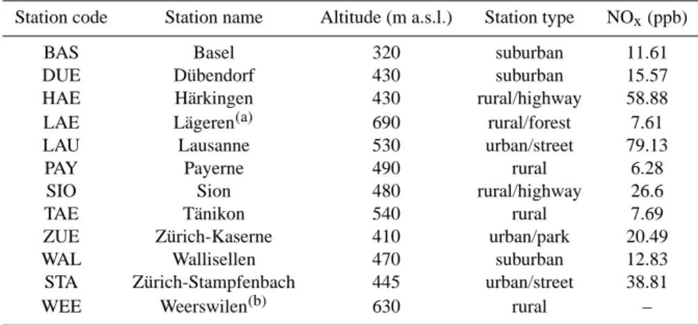
Table 1. Stations used in the analysis. See location of the stations in Fig. 1.

Station code Station name Altitude (m a.s.l.) Station type NOx(ppb)

BAS Basel 320 suburban 11.61 DUE D¨ubendorf 430 suburban 15.57 HAE H¨arkingen 430 rural/highway 58.88 LAE L¨ageren(a) 690 rural/forest 7.61 LAU Lausanne 530 urban/street 79.13 PAY Payerne 490 rural 6.28 SIO Sion 480 rural/highway 26.6 TAE T¨anikon 540 rural 7.69 ZUE Z¨urich-Kaserne 410 urban/park 20.49 WAL Wallisellen 470 suburban 12.83 STA Z¨urich-Stampfenbach 445 urban/street 38.81 WEE Weerswilen(b) 630 rural – WAL, STA and WEE are OSTLUFT stations. The other 9 stations belong to the NABEL network.

The NOxconcentrations in this table correspond to the median of the afternoon averaged NOxlevels during the 1992–2002 period.

(a)_{No NO}

xdata at L¨ageren during the period 22 February–31 October 2000.

(b)_{No NO}

xmeasurements at Weerswilen.

Fig. 1. Location of the stations used in the analysis. See the correspondence between codes and names of the stations in Table 1.

2 Data

2.1 Ozone and NOxmeasurements

Hourly average concentrations of ozone and nitrogen oxides from 12 low-elevation sites of the Swiss air quality monitor-ing network (NABEL) and the eastern cantons of Switzer-land (OSTLUFT) during the period 1 January 1990 to 31 August 2003 were used in this study. The names and loca-tion of the analysed staloca-tions are summarised in Table 1 and Fig. 1. Except Sion, situated in an alpine valley, the sites are

located in the Swiss plateau north of the Alps. At all sta-tions, ozone was measured with the UV absorption method

and nitrogen oxides (NOx)were detected by ozone

chemilu-minescence. NO was directly measured while NO2was first

reduced to NO with a molybdenum converter. The ozone and

NOxmonitors were calibrated automatically every 1–3 days

and manually every 2–4 weeks. In addition, the ozone instru-ments were calibrated every three months with a standard ref-erence photometer, and the molybdenum converter efficiency was examined once a year with gas phase titration (GPT). For more details on data quality assurance of the NABEL

stations see EMPA (2003). Rigorous checks of the ozone

and NOxdata – i.e. analysis of the deviations of the

concen-trations measured at close stations and taking into account the changes in the location of the stations – confirmed that the data quality after 1991 was good for all the sites. Similar results were found in Br¨onnimann et al. (2002). Therefore, the time series of ozone for the 1992–2002 period were anal-ysed in this work.

In this work we analyse the influence of the meteorology on the daily ozone maxima. These maximum concentrations usually occur in the afternoon and are the least affected by local NO sources reacting with ozone to nitrogen dioxide. However, at the most polluted stations (e.g. Lausanne and H¨arkingen) and under more polluted conditions (e.g. win-ter), the effect of the titration on the daily ozone maxima and hence on their trends can be important. To assist in the

interpretation of the results the trends of Ox(sum of O3and

NO2)were also calculated. Ox is not influenced by the

re-action of ozone with NO. However, as mentioned above, the

NO2measurements were performed with molybdenum

con-verters, which exhibit interfering sensitivity to peroxyacyl

ni-trates (PANs), nitric acid (HNO3)and other products of the

oxidation of NOx. The NO2measurements and therefore the

Oxconcentrations are thus upper limits of the real

concentra-tions.

In this analysis, the daily O3and Oxmaxima were defined

as the daily maximum 1-h concentrations measured between 12:00 and 24:00 winter local time (UTC+1 h), and were cal-culated only if at least 9 values (75% of the data) were avail-able for the respective day.

2.2 Meteorological data

Local meteorological data used as explanatory variables in a multiple linear model (see Sect. 3) were taken from the mea-suring NABEL sites and from the closest ANETZ stations operated by MeteoSwiss in the case of the OSTLUFT sta-tions. The parameters sunshine duration and lightning, not measured at the NABEL network, were always taken from the surrounding ANETZ stations. In our analysis we attempt to select explanatory variables to represent the most impor-tant processes that influence ozone in the planetary bound-ary layer (PBL): in situ photochemical production, deposi-tion and vertical mixing. The main parameters measured at those stations are temperature, global radiation, wind speed, wind direction and relative humidity. The morning (6 h to 12 h) and/or afternoon (12 h to 18 h) averages of those mete-orological parameters were calculated when at least 5 out of the 6 hourly values (83% of the data) were available on the respective day.

Under typical summer smog conditions, the daily maxi-mum ozone concentrations and temperature are strongly cor-related. Several statistical models have been suggested to de-scribe the increase in the ozone concentrations with ambient air temperature. Among others, models linear in temperature

after some temporal filtering of both ozone and the meteo-rological variables (Kuebler et al., 2001; Tarasova and Kar-petchko, 2003), a second or higher order polynomial in tem-perature (Br¨onnimann et al., 2002; Bloomfield et al., 1996) or linear regression of the logarithm of daily ozone max-ima with daily maximum temperature as a categorical vari-able (Xu et al., 1996) have been proposed. Scatterplots of the daily ozone maxima against the different meteorological variables used in the analysis suggested that, at least in sum-mer and spring, the afternoon temperature had the strongest relationship to ozone. Moreover, the dependence of ozone on temperature was more quadratic than linear. Therefore, both the afternoon temperature and the square of the afternoon temperature (preceded by a minus sign in the cases when the temperature is negative) have been tested in this study for every station and season. For simplicity, the one which was able to explain more variance was included in the initial model together with the rest of the meteorological variables. The averaged global radiation in the morning and in the after-noon have been used, as solar radiation is the main driver of the photochemical reactions and also affects the vertical mix-ing and thus the dilution of the pollutants, leadmix-ing to lower ozone destruction. The sunshine duration is another param-eter that can be used for the analysis of the influence of the solar radiation on the ozone concentrations. It is defined as the time during which the direct solar radiation exceeds the

level of 120 W/m2. The hourly fraction in which this value is

exceeded was measured at the surrounding ANETZ stations, and both the morning and afternoon averages of this parame-ter were calculated. The morning and afparame-ternoon wind speeds were also used, as these parameters influence the dilution and transport of pollutants. The afternoon wind direction was considered as a discrete variable. It was pooled in two dif-ferent wind sectors for every station – with the exception of three sectors for H¨arkingen – after a careful inspection of the

ozone and NOxlevels for the different wind directions. In

ad-dition, the water vapour mixing ratio whose influence on the ozone concentrations is not so obvious (see Sect. 4.1.1), was calculated and averaged for the afternoon hours. Apart from these meteorological parameters, the day of the week (week-day: Monday–Friday, weekend: Saturday–Sunday) was used to account for the weakly cycle of the anthropogenic emis-sions.

An approximation of the vertical gradient of potential tem-perature in the boundary layer was calculated for all the sta-tions, by using the afternoon temperature at two different al-titude sites in the proximity of the investigated NABEL and

OSTLUFT stations. The parameter Tp, an approximation to

the potential temperature, was calculated from the formula of the dry static energy S (Holton, 1992) for every pair of stations:

Tp=S/Cp=T + gz/Cp, (1)

where Cp = 1005.7 Jkg−1K−1 (dry air), g = 9.81 ms−2, T

difference of Tpbetween the low and the elevated station was

then used as an indicator for dry static stability. In general

there is instability for ∂Tp/∂z<0 (i.e. dTp>0) and stability

for ∂Tp/∂z>0 (i.e. dTp<0), so higher instability is expected

for higher values of dTp. The interpretation of the influence

of this parameter on the ozone concentrations should be done depending on both the season and the character (polluted or rural) of the considered station.

Two parameters which affect the vertical mixing, the dilu-tion of primary pollutants and the deposidilu-tion of ozone within the convective boundary layer (CBL) were calculated daily from the 12:00 UTC radiosoundings at Payerne: the Con-vective Available Potential Energy (CAPE) and the mixing height, which was determined by a simple parcel method (Seibert et al., 2000). The parameters precipitation, close lightning and distant lighting were used to give account for the effect of thunderstorms on the dilution of pollutants. After thunderstorms, the troposphere is usually rather well mixed and the ozone concentrations might reflect similar conditions to background at some stations. In general, the maximum ozone concentrations on a specific day are not only determined by the meteorology on that day but also by the concentrations and meteorology on the previous day. To take into account the meteorology on the previous day, espe-cially the mixing conditions, the absence/occurrence of pre-cipitation and lightning as well as CAPE were used both on the investigated day and on the previous day.

In addition, two parameters from the Alpine Weather Statistics AWS (Wanner et al., 1998) were also used to ac-count for the ozone variations connected with the frontal pas-sages and the synoptic situation. The parameter “number of days after front” was calculated, using the classes 18 and 21 of the AWS, which indicate the presence/absence of a frontal passage – warm front, cold front or occlusion – in Z¨urich on the investigated day. The air is usually well mixed after a frontal passage, and it might be expected that the ozone lev-els build up day by day in summer whereas ozone is more and more depleted under stable conditions in winter. As the effect on the ozone concentrations is more important on the first days, we treated all the days after day 6 in the same way as day 6. Therefore this parameter has 7 possible values: 0, 1, 2, 3, 4, 5, 6. The parameter “synoptic group” is a dis-crete variable that describes 8 different synoptic situations: 3 convective types (anticyclonic, cyclonic and indifferent), 4 advective types based on the 500 hPa wind direction (north, east, south and west) and mixed conditions. Stable situations (“anticyclonic”) are connected with suppressed vertical mix-ing and stagnation of the air masses. The types “cyclonic”, “mixed” and the advective types are usually related to higher vertical mixing and thus favour the dilution of primary pol-lutants. The influence of this parameter on the surface ozone concentrations at 6 NABEL sites was previously investigated in Br¨onnimann et al. (2000).

3 Statistical method

In this study we used a multiple linear model in order to de-scribe the influence of the meteorological variability on the

daily maximum ozone (and Ox)concentrations at the

individ-ual stations. For the selection of the meteorological parame-ters explaining most of the variability in the daily ozone max-ima we used an analysis of covariance (ANCOVA), which allows to include both continuous and discrete variables. All the parameters introduced in Sect. 2.2. were initially used in ANCOVA (for a summary see Table 2). The main as-sumptions of the model are that there is a true underlying linear relationship, that the residuals are mutually indepen-dent with constant variance (homocedasticity) and that the residuals are normally distributed. The meteorological ad-justment of the daily ozone maxima and the calculations of the trends of adjusted daily ozone maxima during the 1992– 2002 period were performed for each station and season sep-arately: spring (MAM), summer (JJA), autumn (SON) and winter (DJF). The winter periods were defined as Decem-ber 1992 to February 1993, . . . , DecemDecem-ber 2002 to Febru-ary 2003. The years 2000 and 2001 were excluded from the analysis for L¨ageren due to missing ozone or meteorological data, mainly as a consequence of destroyed facilities caused by a severe storm.

Although the use of many meteorological parameters in-creases the explained variance, those individual parameters are often correlated to each other, so that irrelevant relations between the meteorological variables and ozone might be in-troduced if all those variables were kept in the final model. As already mentioned, all the variables from Table 2 were initially introduced in a multiple linear model separately for each station and season:

O3(measured)=a1A1+a2A2+...

+b11+b12+b13+... + b21+b22+... + c + ε, (2) where

A1, A2, . . . : continuous variables;

a1, a2, . . . : coefficients of the continuous variables;

b11, b12, b13, . . . , b21, b22, . . . : coefficients or “treatment

effects” of the discrete variables B1, B2, . . . ;

c: intercept;

ε: random error.

A backward elimination procedure performed with the software R (R Development Core Team, 2003) removed the least important predictor variables in different steps. For that purpose, at every step ANCOVA used the F statistics to pro-vide the p-values for the different variables, and the explana-tory variable with the highest p-value (maximum likelihood of having a null coefficient and thus lowest effect on the daily ozone maxima) was removed from the model. A stringent

stopping criterion (p<10−8)was chosen so that a consistent

and not too large set of variables could explain a large frac-tion of the variance in most of the cases. After several it-erations, only the variables satisfying the stopping criterion

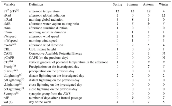
Table 2. Number of stations (out of 12) at which each parameter was selected per season after some ANCOVA iterations. Numbers in italic indicate that the variable was selected for 5 or 6 stations (more than 1/3 of the stations). Numbers in bold indicate that the variable was selected at least for 7 stations (more than half the stations). “N” denotes the seasons in which the variable was not used.

Variable Definition Spring Summer Autumn Winter aT2(aT)(a) afternoon temperature 12 12 12 4 aRad afternoon global radiation 2 0 6 12 mRad morning global radiation 9 8 1 0 aMR afternoon water vapour mixing ratio 9 5 9 5

aSun afternoon sunshine duration 1 0 3 0 mSun morning sunshine duration 2 1 1 1 aWspeed afternoon wind speed 2 1 5 9 mWspeed morning wind speed 0 1 4 3 aWdir(c) afternoon wind direction 3 2 5 4

CBL CBL mixing height 1 0 0 1

CAPE Convective Available Potential Energy 0 0 3 N pCAPE CAPE (on the previous day) 0 0 0 N dTp(b) vertical gradient of potential temperature in the afternoon 1 0 9 9 Precip(c) Precipitation on the investigated day 0 0 7 5

pPrecip(c) precipitation on the previous day 0 0 0 0 dLightning(c) distant lightning on the investigated day 2 2 0 2 pdLigthning(c) distant lightning on the previous day 0 0 0 0 cLightning(c) close lightning on the investigated day 0 0 0 0 pcLightning(c) close lightning on the previous day 0 0 0 0 Synoptic(c) synoptic group from the AWS 0 0 0 0 ndF number of days after a frontal passage 0 9 0 7

wd (c) day of the week 4 0 7 6

Sunshine duration as well as close and distant lighting were taken from the MeteoSwiss ANETZ stations Basel-Binningen (for ozone site BAS), Kloten (DUE), Wynau (HAE), L¨ageren (LAE), Pully (LAU), Payerne (PAY), Sion (SIO), T¨anikon (TAE and WEE), Z¨urich-SMA (ZUE and STA) and Reckenhold (WAL).

(a)_{Either the afternoon temperature or the square of the afternoon temperature was used in the model depending on which one was able to}

explain more variance.

(b)_{The low altitude ANETZ stations used for the calculation of dTp are Basel-Binningen (for BAS), Z¨urich-SMA (LAE, ZUE and STA),}

Payerne (PAY), Sion (SIO), T¨anikon (TAE), Reckenhold (WAL) and G¨uttingen (WEE). For the NABEL stations DUE, HAE and LAU the temperature at low-altitude was taken from the stations themselves. The high altitude ANETZ stations used for the calculation of dTp are L¨ageren (for BAS, DUE, HAE, LAE, TAE, ZUE, WAL, STA and WEE) and Montana (SIO). For LAU and PAY the temperature at high-altitude was taken from the NABEL station at Chaumont.

(c)_{Discrete variables.}

p<10−8were finally included into the multiple linear model

(Eq. 2) for each station and season. Other possible stopping criteria, such us stopping the iterations when the explained variance decreases more than a prescribed value (e.g. 1%) af-ter removing a certain variable from the model, can be found in the statistical literature (e.g. Wilks, 1995). A careful anal-ysis of the residuals revealed that the assumptions of AN-COVA (linearity, homocedasticity and normality) were not violated.

The predicted (i.e. explained by meteorology) daily ozone maxima can be calculated for each station and season with the selected variables and the coefficients obtained from Eq. (2), and the daily ozone maxima can be adjusted for me-teorological effects:

O3 (adjusted)=mean O3+ [O3(measured)−O3(predicted)], (3)

where mean O3: mean of all the considered daily

maxi-mum ozone concentrations measured in the investigated

pe-riod spring, summer, autumn or winter of 1992–2002; O3

(measured): daily maxima of the measured ozone

concen-trations in the investigated period; O3(predicted): modelled

daily maximum ozone concentrations calculated with Eq. (2) for the investigated period

The adjusted daily ozone maxima are thus calculated in Eq. (3) as the mean of the daily ozone maxima in the investi-gated period plus the residuals of the model (Eq. 2).

The trends of the measured and adjusted daily ozone max-ima for the 12 stations and 4 seasons individually can be given by the slopes of the simple linear regression of the re-spective yearly median of the daily ozone maxima against

the year Y:

yearly median [O3(measured)]=d1+d2Y + ε (4)

yearly median [O3(adjusted)]=e1+e2Y + ε. (5)

Each individual yearly seasonal median was considered only if at least 60 daily values were available in the respective year and season to ensure a representative sample size. By using just one value – the yearly median of the daily max-imum ozone concentrations within the same season – per year one can avoid having to take into account the effect of the serial correlation of daily values on the estimation of the standard errors of the coefficients, the number of degrees of freedom and thus the confidence intervals for the slope. Other solutions to the problem of the serial correlation such as reducing the sample size or using autoregressive moving-average (ARMA) models can be found in Wilks (1995) and von Storch and Zwiers (1999).

The procedure explained in this section was also used for

both the meteorological adjustment of the daily Oxmaxima

and the calculation of the trends of their yearly seasonal me-dians. In addition, three slightly different models for the

cal-culation of the daily O3 maxima trends were investigated.

These models and their results will be presented in Sect. 4.3.

4 Results and discussion

4.1 Meteorological adjustment of daily ozone maxima

4.1.1 Influence of meteorological variability on daily ozone

maxima

Table 2 shows all the variables that were initially included in the model as well as the number of stations per season at which they were selected by ANCOVA after some

iter-ations (stopping criterion: p<10−8). Some of the variables

like the mixing height or CAPE derived from the radiosound-ings, lightning, precipitation on the previous day, synoptic group from the AWS or sunshine duration were not incorpo-rated into the final model in most of the cases. Either there is a weak dependence of the daily surface ozone maxima on these parameters or the information given by them was al-ready explained by other meteorological variables.

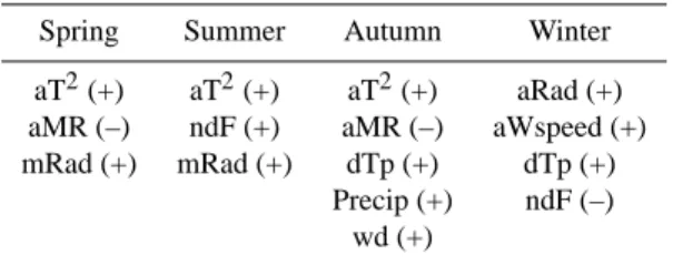
All the variables selected by the model for more than half the stations within the same season are included in Table 3. During the warm seasons the most important explanatory pa-rameters are those that can be related to the chemical ozone production. In particular, the square of the afternoon tem-perature and the morning global radiation presented a pos-itive correlation with daily ozone maxima both in summer and in spring. In general, under typical summer smog con-ditions the daily maximum ozone concentrations and tem-perature are well correlated (e.g. Neftel et al., 2002; Weber and Pr´evˆot, 2002). High temperatures are usually associated

Table 3. Most important explanatory variables for each season. Spring Summer Autumn Winter aT2(+) aT2(+) aT2(+) aRad (+) aMR (–) ndF (+) aMR (–) aWspeed (+) mRad (+) mRad (+) dTp (+) dTp (+)

Precip (+) ndF (–) wd (+)

aT2: square of the afternoon mean temperature (◦C2)

aMR: afternoon water vapour mixing ratio (g/kg) mRad: morning global radiation (W/m2)

aRad: afternoon global radiation (W/m2)

ndF: number of days after a frontal passage

dTp: vertical gradient of potential temperature in the afternoon (◦C)

aWspeed: afternoon averaged wind speed (m/s) Precip: occurrence/absence of precipitation wd: day of the week (weekday or weekend)

(+)/(–) means that ozone is enhanced/reduced for higher values of temperature, global radiation, water vapour mixing ratio or wind speed

Precip (+), wd (+), dTp (+): enhanced ozone for days with precipitation, for weekends and for instability, respectively ndF (+/–): increased/decreased ozone on the following days after a frontal passage

with high radiation and stagnation of the air masses, and both the biogenic emissions and evaporative emissions of anthro-pogenic VOCs increase at high temperatures. In addition, the enhanced thermal decomposition of peroxyacyl nitrates (PANs) at high temperatures yields higher ozone production, as pointed out in some model studies (Sillman and Samson, 1995; Vogel et al., 1999; Baertsch-Ritter et al., 2004). As expected we found a positive correlation between global ra-diation and the ozone concentrations during the warm

sea-sons, as the photolysis of NO2and other compounds like O3,

carbonyls and HONO leads to the formation of radicals with subsequent involvement in ozone production. It is interest-ing that the morninterest-ing radiation and not the afternoon radiation was kept in the final model. This could be partly due to the fact that on fair weather days cumulus clouds often develop in the late afternoon when most of the daily ozone production has already taken place.

In winter, the most important explanatory variables are the ones influencing the vertical mixing and thus the ozone de-struction by titration with NO and dry deposition. Less ozone destruction and thus higher ozone concentrations are ex-pected for high afternoon radiation, high wind speed and in-stability as they favour vertical mixing. In addition, the sup-ply of ozone from the elevated reservoir layer might be en-hanced under good mixing conditions. The model also pre-dicts that in autumn the ozone concentrations are enhanced

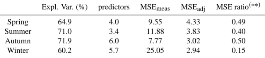
Table 4. Seasonal averages of the explained variance and number of predictors selected per station in the meteorological adjustment (2), MSE

(∗)_{of the regressions of the yearly median of measured (4) and meteorologically adjusted (5) ozone, and MSE ratios – i.e. MSE}

adj/MSEmeas

– for the 12 stations used in the analysis.

Expl. Var. (%) predictors MSEmeas MSEadj MSE ratio(∗∗)

Spring 64.9 4.0 9.55 4.33 0.49 Summer 71.0 3.4 11.88 3.83 0.40 Autumn 71.9 6.0 7.77 3.02 0.50 Winter 60.2 5.7 25.05 2.94 0.15

(∗)_{MSE is an estimate of the variance of the vertical scatter around the fitted line. MSE is given by}

MSE=SSE

n−2,

where SSE is the sum of squared errors in the regressions (4) and (5), and n is the sample size (usually n=11, i.e. 11 years from 1992 to 2002).

(∗∗)_{The MSE ratio was calculated for each station and season and then averaged for the 12 stations within the same season.}

during situations with more vertical mixing and lower pri-mary pollutant concentrations: higher afternoon temperature, instability, precipitation and weekends. Both in autumn and winter, ozone production at higher temperatures or higher ra-diation might contribute to some extent to the meteorologi-cal variability. This is more likely in the autumn season, in which the square of the afternoon temperature is significant for all stations (see Table 2).

The number of days after a frontal passage influences the ozone concentrations in a different way depending on the season: in summer the first days following a frontal passage are usually accompanied by an increase in temperature and more stagnation of the air mass, leading to higher ozone con-centrations day after day; the opposite effect can be observed in winter as the stability favours the ozone loss by titration and dry deposition. The reasons for the negative dependence of ozone on the water vapour mixing ratio in spring and au-tumn are not so obvious, because high water vapour mixing ratios enhance the production of OH radicals yielding higher

ozone concentrations in the high-NOx regime (Vogel et al.,

1999). However, low water vapour might also be connected to less cloudiness and to more vertical mixing.

It is interesting to compare the parameters considered in this study with those from previous analyses. Thompson et al. (2001) summarized the meteorological variables used in the literature for the statistical modelling of ozone. Surface temperature, wind speed and direction, and humidity were included in most models, while solar radiation and pressure were often available but not incorporated into the final mod-els. In contrast, in our study the wind speed and direction were significant at few sites in the warm season although they were more significant in autumn and winter. Moreover, the morning global radiation and the afternoon global radiation were included in the final model for more than half the sta-tions during the warm and cold seasons, respectively (see

Ta-ble 2). Br¨onnimann et al. (2002) considered most of the main parameters used in our analysis and former studies – after-noon mean temperature, global radiation, wind direction and wind speed, relative humidity (similar to water vapour mix-ing ratio, used in our analysis), or day of week – for a regres-sion model of the afternoon ozone peaks in summer (April– September) at 13 NABEL sites. They also included some cir-culation fields – high or low pressure anomalies, zonal flow anomalies and meridional flow anomalies – in their model to account for synoptic scale ozone variations. In addition, they used gradients of both temperature (similar to the pa-rameter “dTp” used in this study) and water vapour mixing ratio at different levels as indicators of stability and air mass changes within and above the boundary layer. However, they eliminated both the circulation fields and the vertical gradi-ents in a second model because of a difficult comparison of results between different sites. Similarly, we used the pa-rameter synoptic group to account for synoptic scale ozone variations although this parameter was not significant in most cases. Our analysis also considered some variables that can be related to stability like lightning, precipitation and two parameters derived from atmospheric soundings (CAPE and mixing height), although they were not significant in most cases either. Only the precipitation and the vertical gradi-ent of potgradi-ential temperature were important at a significant number of stations in autumn and winter, as can be seen in Table 2. In contrast to Br¨onnimann et al. (2002) and our anal-ysis, Kuebler et al. (2001) first removed the long-term trend as well as the seasonal and weekly variations in their analysis of the summer (May–October) peak ozone concentrations at 12 NABEL sites. As a consequence, only three meteorolog-ical parameters – the afternoon mean temperature, the daily solar radiation and the afternoon mean wind speed – were needed to remove the residual short-term variations by us-ing a multiple linear regression model. Unlike Kuebler et

al. (2001) and Br¨onnimann et al. (2002) that focused on the trend analysis of summer smog ozone in Switzerland, this study has analysed the variability of daily ozone maxima in the four seasons. Our study has also found that the num-ber of days after a frontal passage, variable not considered in former studies, is important to account for the ozone genera-tion (summer months) or destrucgenera-tion (winter months) after a frontal passage.

4.1.2 Model performance

The explained variance averaged over all stations ranged from 60.2% in winter to 71.9% in autumn (see Table 4). In general, the number of significant explanatory variables was higher in the cold months, due to the importance of local effects in winter – on average 5.7 predictors were used at ev-ery station for the meteorological adjustment of daily ozone maxima during this season – and the more variable meteo-rology in autumn – on average 6 predictors were needed. In

contrast, most of the variability in the summer daily O3

max-ima was explained by the afternoon temperature, the morning global radiation and the number of days after front (see Ta-bles 2 and 3). On average only 3.4 parameters were needed in summer and 4 in spring.

Another way of assessing the model performance is to test if the year-to-year variability in the daily maximum ozone concentrations is effectively reduced after the meteorologi-cal adjustment. For that purpose, we meteorologi-calculated the mean-squared error (MSE) of the regressions of the yearly sea-sonal medians of both the measured and adjusted daily ozone

maxima against the year (Eqs. 4 and 5), giving MSEmeasand

MSEadj, respectively. The mean-squared error is given by

MSE = SSE

n −2, (6)

where SSE is the sum of squared errors in a simple linear regression and n is the sample size. This parameter indi-cates the degree to which the distribution of residuals clusters tightly (small MSE) or spreads widely (large MSE) around

the regression line (Wilks, 1995). MSEmeas and MSEadj

were calculated for each station and season, and their sea-sonal means are given in Table 4. There is high variabil-ity in the yearly medians of the measured daily ozone max-ima for most of the stations and seasons (see the high

val-ues of the seasonal averages of MSEmeas in Table 4). This

variability is reduced after the meteorological adjustment as

can be seen from the lower values of MSEadj and thus low

(MSEadj/MSEmeas) ratios. On average, after the

meteoro-logical adjustment MSE is reduced by 85% in winter, 60% in summer, and 50% in autumn and spring. At T¨anikon as an example the yearly medians of the daily maximum ozone concentrations usually lie closer to the trend line after the meteorological adjustment (Fig. 2).

1992 1994 1996 1998 2000 2002 40 45 50 55 year meas. ozone [ppb] TAE Spring 1992 1994 1996 1998 2000 2002 40 45 50 55 year adj. ozone [ppb] 1992 1994 1996 1998 2000 2002 55 60 65 year meas. ozone [ppb] TAE Summer 1992 1994 1996 1998 2000 2002 55 60 65 year adj. ozone [ppb] 1992 1994 1996 1998 2000 2002 25 30 35 year meas. ozone [ppb] TAE Autumn 1992 1994 1996 1998 2000 2002 25 30 35 year adj. ozone [ppb] 1992 1994 1996 1998 2000 2002 15 20 25 30 35 year meas. ozone [ppb] TAE Winter 1992 1994 1996 1998 2000 2002 15 20 25 30 35 year adj. ozone [ppb]

Fig. 2. Yearly medians of the measured daily ozone maxima and meteorologically adjusted daily ozone maxima at T¨anikon for all seasons during 1992–2002. The calculated MSE ratio (MSE_adj/MSEmeas) for this station is 0.24 in spring, 0.10 in

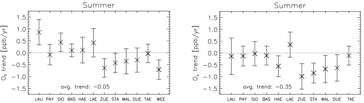
Fig. 3. Trends of the seasonal medians of the meteorologically adjusted daily maximum O₃(left) and Ox(right) concentrations during

1992–2002. Uncertainty estimates represent 95% confidence intervals. The averaged trend for all the stations in every season is shown at the lower part of each plot. Station codes (see corresponding names in Table 1) on the x-axis are ordered according to their geographical longitude from West to East. The Oxtrend was not calculated for Weerswilen (WEE) as there were no NOxmeasurements at this station.

Fig. 4. Trends of the 90th percentiles of the meteorologically adjusted daily maximum O3(left) and Ox(right) concentrations during summer

1992–2002. Uncertainty estimates represent 95% confidence intervals.

4.2 Trends of meteorologically adjusted daily O3 and Ox

maxima

The trends of the seasonal medians of adjusted daily O3

max-ima – calculated with the model (Eq. 5) – and Ox maxima

– calculated analogously – for each station and season are shown in the left- and right-hand side plots of Fig. 3, respec-tively. The uncertainty estimates in the plots represent the 95% confidence intervals for those trends.

The absence of negative trends for daily ozone maxima at most stations in spring and summer, seasons in which the main driving mechanism is photochemical production, suggests that the emission reductions of primary pollutants

during the 90s – 39% for NOx and 49% for NMVOC in

Switzerland during the 1990–2002 period (Vestreng et al., 2004) – were insufficient to significantly reduce the daily maximum ozone concentrations. This was previously found in Kuebler et al. (2001) for the high percentiles of ozone in summer (May-October) 1985–1998. At the 6 most pol-luted stations used in the analysis (those with the highest

NOx levels in Table 1), we observed an average decrease

in the measured afternoon NOx concentrations of 30% in

summer and 35% in winter during the 1992–2002 period.

Positive although not statistically significant O3trends were

observed in summer, except for four stations in the region around Z¨urich (Z¨urich-Kaserne, Z¨urich-Stampfenbach,

Wal-lisellen and Weerswilen). The positive O3trends might be

related to the lower effect of the O3loss by titration through

NO as a consequence of the decreased emissions of primary pollutants during the 90s. The effect of titration is espe-cially important at the most polluted sites. On average, the

Oxtrends are around 0.3 ppb yr−1lower than the O3trends

for all stations and seasons, which confirms that the

calcu-lated O3trends were affected by the reduced effect of

titra-tion. However, except for the mentioned stations in the

re-gion around Z¨urich, the Ox trends are slightly negative or

positive but not significant in summer. The trend analysis of the seasonal 90th percentiles of the meteorologically

ad-justed daily O3and Oxmaxima (Fig. 4) provided additional

information: downward trends in summer Oxwere found for

5 stations in the region around Z¨urich (on average −0.73 ppb

yr−1_{for H¨arkingen, Z¨urich-Kaserne, Z¨urich-Stampfenbach,}

Wallisellen and D¨ubendorf) as well as a significant

down-ward trend in summer O3observed at Weerswilen (the Ox

trend was not calculated for this station as no NOx

mea-surements were available). The summer O3 and Ox trends

at L¨ageren are higher for the 90th percentiles than for the medians, although we should keep in mind that the trends calculated at this station can be affected by the exclusion of two years from the analysis (2000 and 2001) as explained in Sect. 3. As the region around Z¨urich is the most densely pop-ulated and industrialised area in Switzerland, the local pro-duction is contributing more to the ozone concentrations than in other areas. The decrease of the precursor emissions thus might have led to a significant decrease of ozone only in this area, and that decrease is more pronounced for the highest ozone peaks on summer smog days. Considering the results found for all the analysed stations, the lower regional ozone production due to the decreased emissions of ozone precur-sors might have been compensated by increased large-scale background or other processes.

Significantly positive trends of the medians of adjusted daily ozone maxima were found for all the stations in au-tumn and winter – except at Weerswilen in auau-tumn –, prob-ably due to the reduced effect of the titration on the ozone concentrations. As already mentioned, this effect could be

confirmed by the lower trends of daily Oxmaxima (on

av-erage 0.39 ppb yr−1 _{in winter) compared to the trends of}

daily ozone maxima (on average 0.69 ppb yr−1 _{in winter).}

The Ox trends are also significantly positive at most of the

stations, suggesting an increase in background ozone as al-ready proposed by Br¨onnimann et al. (2002). There are ev-idences for an increase of the mean ozone concentrations in Europe at high-altitude sites (e.g. for Zugspitze see Guicherit and Roemer, 2000, and TOR-2, 2003), at lower altitude sites under selected background conditions (e.g. for Switzerland

see Br¨onnimann et al., 2000) or at remote sites (e.g. for Mace Head see Simmonds et al., 2004). Nevertheless, the causes for this increase need further study since “background ozone” is influenced by different chemical and dynamical processes on different scales, such as photochemistry on a continental and on a hemispheric scale as well as large- or regional scale horizontal and vertical transport.

Lausanne, the most polluted site analysed in this study, is the only station that presents significantly positive trends of adjusted daily ozone maxima during all seasons. This is most

probably due to the reduced effect of the O3titration by NO.

In fact, the Oxtrends at this station are very close to zero in

all seasons except in winter (0.49±0.32 ppb yr−1). However,

when analysing the Ox trends at such polluted stations like

Lausanne and H¨arkingen, one should take into account that

those trends are affected by the trend in NO2emissions. The

dominant NOx source in urban locations is road traffic

ex-haust. Although the NO2input from direct emission varies

from one location to another or from one time to another, as a result of varying vehicle fleet composition and driving speeds, an average figure of approximately 5% (by volume)

of NOxemitted in the form of NO2is often quoted (Clapp

and Jenkin, 2001). If we assume that the 5% value is constant for the studied period, it is possible to estimate the trend of

emitted NO2as the 5% of the NOxtrend (in ppb yr−1). As an

example the calculated trend of NOxat Lausanne is around

−4.7 ppb yr−1(around 44%, somewhat higher than the 32%

value given by the emission inventory for Switzerland in that

period), resulting in a trend of directly emitted NO2lower

than −0.25 ppb yr−1. This effect is not significant as the

95% confidence intervals for the Ox trends at all sites are

always larger than the absolute value of the calculated trends

of directly emitted NO2.

4.3 Robustness of the model

Three variations of the model described in Sect. 3 were used and their results were compared to those of the first model. This made it possible to investigate the sensitivity of both the meteorological adjustment of daily ozone maxima and the calculated trends of adjusted daily ozone maxima to the model chosen.

As already explained in Sect. 3, the statistical model was optimised so that a consistent and not too large set of ex-planatory variables was kept in the final model in most cases. Actually, there was high consistency in the selection of ex-planatory variables for the different sites within the same season although each station presented its own distinctive patterns. A “reduced model” was used to address whether a more limited number of parameters could be consistently used for all the stations within the same season. For that pur-pose, only the most important explanatory variables in ev-ery season – i.e. variables from Table 3 – were included in the model (Eq. 2) for the calculation of the predicted daily ozone maxima at every station and the corresponding

sea-sonal trends of adjusted daily ozone maxima were also cal-culated with Eq. (5). In general, the results obtained with the “reduced model” are very similar those of the first model (see

columns “yearly median O3” and “reduced model” in

Ta-ble 5) although somewhat poorer – usually lower explained variance, occasionally different trends and sometimes larger confidence intervals – for some stations in some seasons. This suggests that, although it is preferable to use the model described in Sect. 3, the “reduced model” can be used if a simplified and consistent procedure for all stations is wanted. Finally, in a different approach, the year Y was included as an additional variable together with the rest of the meteo-rological parameters (those from Table 2) in the multilinear model:

O3(measured)=mY + α1A1+α2A2+...

+β11+β12+β13+... + β21+β22+... + c + ε. (7) As in the meteorological adjustment explained in Sect. 3, a backward elimination procedure was used to remove the least important predictor variables from the model (Eq. 7). For that purpose, the least significant explanatory variable (high-est p-value) was also provided by ANCOVA at every step

and the same stopping criterion (p<10−8)was used. The

variable year (Y) was not allowed to be removed from the model (Eq. 7) so that the trend – significant or not – could be calculated. The coefficient m obtained after all the iterations is in this case the new value of the trend and can be

com-pared with the trends e2obtained from Eq. (5) and f2from

the linear model:

yearly mean [O3 (adjusted)]=f1+f2Y + ε. (8)

For every station and season, very similar explanatory vari-ables were finally kept in the initial meteorological adjust-ment (Eq. 2) and in the model (Eq. 7). In general, the

cal-culated ozone trends e2, f2and m for each station and

sea-son did not differ either. This suggests that the selection of the model is not too critical either for the meteorologi-cal adjustment or for the meteorologi-calculation of the trends of daily ozone maxima. A short summary with the comparison of the averaged seasonal trends obtained with the different mod-els is presented in Table 5. However, the model (Eq. 7) presents the drawback that it only gives a value of the trend, whereas the other methods allow for an easier visual inspec-tion of the yearly seasonal medians/means of the adjusted daily ozone maxima. A visual inspection of the fitted linear trend makes it possible to identify years with very high/low ozone maxima that can have a strong impact on the calcula-tion of a linear trend, especially when those years are located at the beginning or end of the considered period. As seen in Sect. 4.1.2, if the regression of the yearly median or yearly mean of daily ozone maxima against the year is used, one can also compare the year-to-year variability (MSE values) of daily ozone maxima before and after the meteorological adjustment.

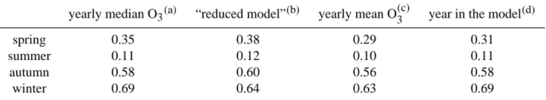
Table 5. Averages of the trends in the seasonal medians of adjusted daily ozone maxima calculated with the different models for the 12 stations in Table 1. The trends are expressed in ppb yr−1.

yearly median O3(a) “reduced model”(b) yearly mean O(₃c) year in the model(d)

spring 0.35 0.38 0.29 0.31 summer 0.11 0.12 0.10 0.11 autumn 0.58 0.60 0.56 0.58 winter 0.69 0.64 0.63 0.69

(a)_{The individual trends of the yearly median of daily O}

3maxima at every station were calculated with Eq. (5).

(b)_{For the calculation of the daily O}

3 maxima trends with the “reduced model” the Eq. (5) was also used but only the most important

explanatory variables in every season – i.e. variables from Table 3 – were first consistently introduced in Eq. (2) for the meteorological adjustment of ozone at all the stations.

(c)_{The individual trends of the yearly mean of daily O}

3maxima were calculated with Eq. (8).

(d)_{The O}

3trends calculated with the year included in the model are given by the coefficient of the year in the regression model (Eq. 7).

5 Analysis of an extreme case: summer 2003

Summer 2003 was extremely dry and warm in Europe. Based on a reconstruction of monthly and seasonal temperature fields for European land areas back to 1500, Luterbacher et al. (2004) concluded that summer 2003 was very likely warmer than any other summer during the last 500 years. In a large area of central Europe, including Switzerland, the mean summer (June, July and August) temperatures exceeded the

1961–1990 mean by ∼3◦_{C, corresponding to an excess of}

up to 5 standard deviations of the summer means in that pe-riod (Sch¨ar et al., 2004). Taking into account the tempera-ture record of the past ∼150 years, such a warm summer is a very rare event, even when the warming in the last decades is considered. The described summer 2003 led to unusu-ally long periods with high ozone concentrations in Switzer-land: on average the number of exceedances of the Swiss

air quality standard for 1-h mean values (120 µg/m3)was up

to 700 h, twice as much as in the previous years. Moreover, the 2003 summer mean of the daily ozone maxima at the in-vestigated stations exceeded the 1992–2002 summer mean of daily ozone maxima by more than 15 ppb, corresponding to 5 standard deviations of those 1992–2002 summer means, sim-ilarly as found for the temperature. The effects of the sum-mer 2003 heat wave were also observed in other European countries. The UK Office for National Statistics reported an excess of 2045 deaths in England and Wales for the period from 4 to 13 August 2003 above the 1998–2002 average for that time of the year. Stedman (2004) estimated that between 423 and 769 of those excess deaths (21–38% of the total)

were associated with the elevated ambient ozone and PM10

concentrations. In a similar study Fischer et al. (2004) found that of an excess of 1000–1400 deaths in the Netherlands dur-ing summer 2003 compared to the average summer of 2000,

400–600 deaths were ozone- and PM10-related.

In order to assess whether the statistical model described in Sect. 3 was able to explain the high ozone concentrations

in Switzerland during that extreme summer, the coefficients calculated with Eq. (2) for each station during the period summer 1992–2002 were also used for the calculation of the predicted daily ozone maxima at the corresponding station in summer 2003. The meteorologically adjusted daily ozone maxima for the period summer 1992–2003 were calculated with Eq. (3).

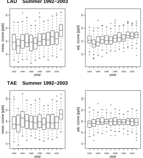
A visual inspection of the yearly medians of the daily ozone maxima at the different stations in summer (Fig. 5) reveals that the very high median of the measured daily max-ima in summer 2003 (“meas. ozone” plots) is reduced af-ter the meteorological adjustment (“adj. ozone” plots) for most of the stations, with the exception of H¨arkingen (pol-luted station close to a highway), for which the meteoro-logical adjustment was less effective. One reason for this might be that the excess of the mean daily ozone maxima observed at this station in summer 2003 (over 20 ppb and 7 standard deviations higher than in summer 1992–2002) is larger than at the other stations. Not only the medians of the daily maximum ozone concentrations but also the variability of the daily ozone maxima in summer 2003 are consistent with the previous years after adjusting for the meteorological influence. Examples are shown for an urban site – Lausanne – and a rural one – T¨anikon – in Fig. 6. Very similar results were obtained for the rest of the stations, again with the ex-ception of H¨arkingen.

The fact that the meteorological adjustment introduced in Sect. 3 also performs well for an extreme case like that of summer 2003 also indicates that our former conclusions about the main explanatory variables are robust. Consider-ing the afternoon temperature, the number of days after a frontal passage and the morning global radiation for most of the stations (see column “Summer” in Table 2), in combina-tion with only one or a few variables which vary depending on the station (on average only 3.4 predictors are needed, as seen in Table 4), one can explain the meteorological variabil-ity of summer daily ozone maxima at different sites north

1992 1994 1996 1998 2000 2002 45 50 55 60 65 70 75 80 BAS Summer 1992−2003 year meas. ozone [ppb] 1992 1994 1996 1998 2000 2002 45 50 55 60 65 70 75 80 year adj. ozone [ppb] 1992 1994 1996 1998 2000 2002 50 55 60 65 70 75 DUE Summer 1992−2003 year meas. ozone [ppb] 1992 1994 1996 1998 2000 2002 50 55 60 65 70 75 year adj. ozone [ppb] 1992 1994 1996 1998 2000 2002 40 45 50 55 60 65 70 HAE Summer 1992−2003 year meas. ozone [ppb] 1992 1994 1996 1998 2000 2002 40 45 50 55 60 65 70 year adj. ozone [ppb] 1992 1994 1996 1998 2000 2002 55 60 65 70 75 LAE Summer 1992−2003 year meas. ozone [ppb] 1992 1994 1996 1998 2000 2002 55 60 65 70 75 year adj. ozone [ppb] 1992 1994 1996 1998 2000 2002 30 35 40 45 50 55 60 LAU Summer 1992−2003 year meas. ozone [ppb] 1992 1994 1996 1998 2000 2002 30 35 40 45 50 55 60 year adj. ozone [ppb] 1992 1994 1996 1998 2000 2002 50 55 60 65 70 75 PAY Summer 1992−2003 year meas. ozone [ppb] 1992 1994 1996 1998 2000 2002 50 55 60 65 70 75 year adj. ozone [ppb] 1992 1994 1996 1998 2000 2002 50 55 60 65 SIO Summer 1992−2003 year meas. ozone [ppb] 1992 1994 1996 1998 2000 2002 50 55 60 65 year adj. ozone [ppb] 1992 1994 1996 1998 2000 2002 55 60 65 70 75 TAE Summer 1992−2003 year meas. ozone [ppb] 1992 1994 1996 1998 2000 2002 55 60 65 70 75 year adj. ozone [ppb] 1992 1994 1996 1998 2000 2002 45 50 55 60 65 70 75 ZUE Summer 1992−2003 year meas. ozone [ppb] 1992 1994 1996 1998 2000 2002 45 50 55 60 65 70 75 year adj. ozone [ppb] 1992 1994 1996 1998 2000 2002 50 55 60 65 70 75 WAL Summer 1992−2003 year meas. ozone [ppb] 1992 1994 1996 1998 2000 2002 50 55 60 65 70 75 year adj. ozone [ppb] 1992 1994 1996 1998 2000 2002 50 55 60 65 70 STA Summer 1992−2003 year meas. ozone [ppb] 1992 1994 1996 1998 2000 2002 50 55 60 65 70 year adj. ozone [ppb] 1992 1994 1996 1998 2000 2002 50 55 60 65 70 WEE Summer 1992−2003 year meas. ozone [ppb] 1992 1994 1996 1998 2000 2002 50 55 60 65 70 year adj. ozone [ppb]

Fig. 5. Yearly medians of the daily ozone maxima at the analysed stations in summer for the 1992–2003 period. For every station the first plot shows the yearly medians of the measured daily ozone maxima and the second plot depicts the yearly medians of the adjusted daily ozone maxima. The trend lines in the plots have been calculated using only summer data from 1992 to 2002.

1992 1994 1996 1998 2000 2002 20 40 60 80 year meas. ozone [ppb]

LAU Summer 1992−2003

TAE Summer 1992−2003

Fig. 6. Boxplots of the measured (left) and meteorologically adjusted (right) daily ozone maxima in summer 1992–2003 for Lausanne (top) and T¨anikon (bottom). Each box depicts the central half of the data between the lower quartile (q0.25)and the upper quartile (q0.75). The

line across the box displays the median value (q0.5). The whiskers extend from the top and the bottom of the box to depict the extent of the

main body of the data. Extreme data values are plotted with a circle.

of the Alps in Switzerland even during this extremely warm summer.

6 Conclusions

An analysis of covariance (ANCOVA) has been used to ac-count for the variability of daily ozone maxima at 12 stations north of the Alps in Switzerland during the 1992–2002 pe-riod. The analysis has been done separately for each season, motivated by the well known fact that the processes govern-ing the relations between ozone and meteorological parame-ters differ significantly during the year and can even change sign (Tarasova and Karpetchko, 2003). The analysis of the most important explanatory variables (see Tables 2 and 3) leads to the conclusion that ozone production is the dom-inant mechanism both in summer and spring, while ozone destruction by titration and dry deposition prevails in winter, as expected. Autumn seems to be an intermediate case, with

more variable meteorology, and around 6 parameters are usu-ally needed to account for the meteorological variability of daily ozone maxima in this season compared to the average of 3.5 parameters in summer. In general, similar meteorolog-ical variables to those reported in the literature for the mete-orological adjustment of ozone in the summer season were found to be significant for the same season in this work. In addition, this analysis found that the number of days after a frontal passage, a variable not considered in previous studies, is important to account for ozone generation in summer and ozone destruction in winter.

Most of the variability in the daily maximum ozone con-centrations was explained by ANCOVA, taking into account the meteorological variability on a local, regional and to some extent synoptic scale. On average, the explained vari-ance ranged from 60.2% in winter to 71.9% in autumn. The year-to-year variability of the daily ozone maxima was re-duced by 85% in winter, 60% in summer, and 50% in autumn and spring after the meteorological adjustment.

No significant downward trends in either the seasonal

me-dians or the 90th percentiles of daily O3/Ox maxima were

found for 6 stations in summer. However, 6 sites in the indus-trialised region around Z¨urich presented significant

down-ward trends in the summer 90th percentiles of daily Ox or

O3maxima, which suggests that the precursor emission

re-ductions had at least a significant effect on the highest ozone peaks during summer smog days in this area. At all loca-tions, the decrease in the local production due to the

reduc-tions of the precursor emissions – 39% for NOx and 49%

for NMVOC in Switzerland during the 1990–2002 period (Vestreng et al., 2004) – might have been compensated by a background ozone increase. The significantly positive trends

of O3 in winter (on average 0.69 ppb yr−1) are partially

due to the lower titration as a consequence of the decreased emissions, too. The influence of the chemistry on a local

and regional scale is lowered if one analyses the Oxwinter

trends. The increase of Oxfound for most of the stations in

autumn (on average 0.23 ppb yr−1)and winter (on average

0.39 ppb yr−1)could be due to increasing background ozone

levels, in agreement with other studies for Europe (TOR-2 and TROTREP) and Switzerland (Br¨onnimann et al., 2000, 2002). The causes for this European background increase might be related to intercontinental transport, hemispheric background increase or large-scale meteorological variabil-ity not taken into account by local meteorological factors. The impact of some of these processes on the surface ozone variability and trends have been addressed, among others, by Lelieveld and Dentener (2000) and Tarasova et al. (2003).

Finally, summer 2003, the warmest summer in the long-term temperature series available in Switzerland since 1864, was a good opportunity to validate our model. The daily ozone maxima in summer 2003 were on average 15 ppb higher than in summer 1992–2002, corresponding to 5 stan-dard deviations of the summer means of daily ozone max-ima in that period. The model used to adjust for meteoro-logical effects was able to lower the daily ozone maxima in that summer to concentrations found in the previous years. Even though an event like that of summer 2003 is statisti-cally extremely unlikely if one takes into account the climate in the last ∼150 years, regional climate model (RCM) simu-lations in scenarios with increased atmospheric greenhouse-gas concentrations suggest that such summers might be more frequent in Europe towards the end of the century (Sch¨ar et al., 2004). This might lead to a higher occurrence of severe ozone episodes with serious implications for human health (e.g. see Fischer et al., 2004; Stedman, 2004) and ecosys-tems if the emissions are not significantly reduced.

Acknowledgements. This research was carried out with the

financial support of the Swiss Agency for Environment, Forests and Landscape (SAEFL). The meteorological data from ANETZ stations and the Payerne soundings were provided by MeteoSwiss. Ozone and primary pollutants data at Z¨urich-Stampfenbach, Wallisellen and Weerswilen were provided by OSTLUFT. The authors gratefully acknowledge W. Stahel, B. Tona, J. Maeder and

S. Br¨onnimann – ETH Z¨urich – for helpful discussions concerning the statistical methods used. We also thank two anonymous reviewers for their interesting comments, which helped to improve the quality of the manuscript.

Edited by: A. Hofzumahaus

References

Baertsch-Ritter, N., Keller, J., Dommen, J., and Pr´evˆot, A. S. H.: Effects of various meteorological conditions and spatial emission resolutions on the ozone concentration and ROG/NOxlimitation

in the Milan area (I), Atmos. Chem. Phys., 4, 423–438, 2004, SRef-ID: 1680-7324/acp/2004-4-423.

Bloomfield, P. J., Royle, J. A., Steinberg, L. J., and Yang, Q.: Ac-counting for meteorological effects in measuring urban ozone levels and trends, Atmos. Envir., 30 (17), 3067–3077, 1996. Br¨onnimann, S., Schuepbach, E., Zanis, P., Buchmann, B., and

Wanner, H.: A climatology of regional background ozone at dif-ferent elevations in Switzerland (1992–1998), Atmos. Envir., 34, 5191–5198, 2000.

Br¨onnimann, S., Buchmann, B., and Wanner, H.: Trends in near-surface ozone concentrations in Switzerland: the 1990s, Atmos. Envir., 36, 2841–2852, 2002.

Clapp, L. J. and Jenkin, M. E.: Analysis of the relationship between ambient levels of O₃, NO₂and NO as a function of NOxin the

UK, Atmos. Envir., 35 (36), 6391–6405, 2001.

Cox, W. and Chu, S.: Assessment of interannual ozone variation in urban areas from a climatological perspective, Atmos. Envir., 30, 2615–2625, 1996.

Davis, J. M., Eder, B. K., Nychka, D., and Yang, Q.: Modeling the effects of meteorology on ozone in Houston using cluster anal-ysis and generalized additive models, Atmos. Envir., 32, 2505– 2520, 1998.

Dommen, J., Neftel, A., Sigg, A., and Jacob, D. J.: Ozone and hydrogen peroxide during summer smog episodes over the Swiss Plateau: Measurements and model simulations, J. Geophys. Res., 100, 8953–8966, 1995.

Dommen, J., Pr´evˆot, A. S. H., Hering, A. M., Staffelbach, T., Kok, G. L., and Schillawski, R. D.: Photochemical production and aging of an urban air mass, J. Geophys. Res., 104, 5493–5506, 1999.

Ehhalt, D., Prather, M., Dentener, F., Derwent, R., Dlugokencky, E., Holland, E., Isaksen, I., Katima, J., Kirchhoff, V., Matson, P., Midgley, P., Wang, M., et al.: Atmospheric Chemistry and Greenhouse Gases, in: Climate Change 2001: The Scientific Ba-sis, edited by: Houghton, J. T., Ding, Y., Griggs, D. J., et al., Contribution of Working Group 1 to the Third Assessment Re-port of the IPCC, 4, 239–288, 2001.

EMPA (Swiss Federal Laboratories for Materials Testing and Re-search): Technischer Bericht zum Nationalen Beobachtungsnetz F¨ur Luftfremdstoffe (NABEL) 2002, D¨ubendorf, 2003. Fischer, P. H., Brunekreef, B., and Lebret, E.: Air pollution related

deaths during the 2003 heat wave in the Netherlands, Atmos. En-vir. 38, 1083–1085, 2004.

Guicherit, R. and Roemer, M.: Tropospheric ozone trends, Chemo-sphere – Global Change Science, 2, 167–183, 2000.

Holton, J. R.: An Introduction to Dynamic Meteorology, 3rd edi-tion, Academic Press, 1992.