Application Of Rayleigh's Principle To Guided Waves In A Borehole

GUIDED WAVES IN A BOREHOLE

by

K.J. Ellefsen and C.H. Cheng Earth Resources Laboratory

Department of Earth, Atmospheric, and Planetary Sciences Massachusetts Institute of Technology

Cambridge, MA 02189

ABSTRACT

The Lagrangian for guided waves in a completely general borehole model is presented. Rayleigh's principle is used to derive the first order perturbations in wavenumber and frequency due to slight perturbations in the physical properties of the model. The principle is also used to calculate perturbations in frequency due to perturbations in wavenumber. These formulas are applied to a fluid-filled borehole through an infinite, transversely isotropic formation, for which the axis of symmetry is aligned with the borehole, to calculate (1) partial derivatives of wavenumber and velocity at constant frequency, (2) partial derivatives of frequency and velocity at constant wavenumber, and (3) group velocity. These formulas are also applied to a formation with general anisotropy to calculate the velocity dispersion.

INTRODUCTION

The transversely isotropic character of many sedimentary rocks, which has important implications for hydrocarbon exploration and production, can be studied using the guided waves generated by acoustic logging tools. Because the transverse isotropy principally affects the velocity dispersion of the guided waves, the dispersion curves can be used to estimate the elastic properties of the formation. This estimation requires partial derivatives of the phase velocity with respect to the elastic moduli, and, because numerical differentiation can frequently yield inaccurate results, analytical expressions for the derivatives are usually sought.

Several groups of investigators have used Rayleigh's principle to calculate partial derivatives for tube and pseudo-Rayleigh waves in isotropic formations. Cheng et al. (1982) used partition coefficients, which are derived from the partial derivatives, to determine P- and S-wave attenuation from the tube and pseudo-Rayleigh waves. Toksoz et al. (1984) used the partial derivatives to calculate group velocity. Stevens

and Day (1986) used the Cheng et aI. (1982) formulation for the partition coefficients to estimate the S-wave velocity in slow formations. Burns and Cheng (1987) derived partition coefficients for boreholes with multiple, radial layers and used the coefficients to evaluate the effects of formation properties upon phase velocity and attenuation.

The first purpose of this paper is to derive analytical expressions for the partial derivatives for all guided waves in transversely isotropic formations. Rayleigh's prin-ciple will be used to derive the derivatives of phase velocity at constant frequency and at constant wavenumber. The equations for the partial derivatives are general and can be applied to a borehole with multiple, radial layers. The use of the equations will be demonstrated by calculating partial derivatives, partition coefficients, and group ve-locity for waves travelling along a fluid-filled borehole through an infinite, transversely isotropic formation.

Before an inversion using the velocity dispersion curves is attempted, the effects of a slightly anisotropic formation should be assessed. This topic has not been stud-ied thoroughly in borehole seismology. However, in earthquake seismology, Smith and Dahlen (1973) used Rayleigh's principle to estimate the perturbations in surface wave phase velocity due to anisotropy in the crust and upper mantle. For the earth's nor-mal modes, Woodhouse and Dahlen (1978) used this principle to derive equations for perturbations in frequency due to changes in densities, elastic constants, locations of boundaries, and many other properties.

The second purpose of this paper is to determine the first order effects of a slightly anisotropic formation upon the phase velocity of the guided waves. The expressions for the velocity perturbations are based upon Rayleigh's principle and can be applied to a borehole with multiple, radial layers. These equations are used to calculate the phase velocities of guided waves traveling along a fluid-filled borehole through an infinite, slightly anisotropic formation.

RAYLEIGH'S PRINCIPLE

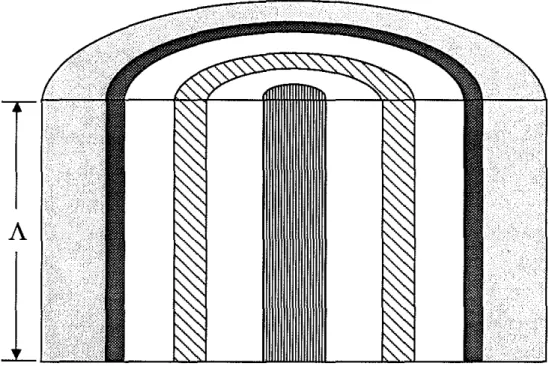
The borehole model consists of multiple layers each of which may be either a perfectly elastic solid or an inviscid fluid (Figure 1). Locations in the model are defined with respect to a circular cylindrical coordinate system for which the z axis is in the bore-hole's center. Each layer is concentric with and extends to infinity along the z axis; the outermost layer extends to infinity in the radial direction. Each layer is homogeneous and is characterized by its density, p, and elastic moduli, Cijkl.

The boundary conditions must be established for guided wave propagation. Of the entire borehole model (Figure 1), only a volume element, V, having a thickness of one wavelength, A, is needed because wave propagation in every volume element is the

same. Within the volume element surfaces are found between the layers, at the end faces, and at infinite radius. The normal to any surface is ni. The boundary between two solid layers is welded meaning that the displacements, Ui, and tractions, Ti, are continuous: [Ui]~ [Td~ =

0

o

(1)

(2)

The notation, ['J~, indicates the change in the quantity across the boundary. At a fric-tionless boundary, which occurs between fluid and solid layers, the normal component of displacement is continuous:

[niUi]~= 0 ,

and the traction is continuous and normal to the boundary:

[Ti]~ 0

Ti = n,[Tjnj]

(3)

(4)

(5)

Applying Hamilton's principle to the guided waves in the borehole will simplify the derivation of Rayleigh's principle. The Lagrangian energy is defined as the kinetic energy minus the elastic strain energy:

1

t+7

8 , dtL =

L =

_Jv

r

dV

(~pu.u.

_{2 t t} -

~u'

_{2 ),t}'C"kIU/ k)_{1,) I}

in which Ui and U/,k indicate differentiation with respect to time and space. averaging the Lagrangian energy over one period, T, its variation is calculated.

81'+7 dt_t

_J

r

dV

(~pu,u,

-

~u'

'C"kIU/k)

v

2 t t 2 3,t 1) I

=

1'+7

dt

fv

dV (PUi

a~~i

- 8Uj,iCijklUl,k)

(6) After

(7)

Integration by parts is applied to the temporal derivatives, and Gauss's theorem to the spatial derivatives.

1

,+7

8, dtL

=

fv

dV pUi8ui

1:+7_[+7

dt

fv

dV(pUi - Tji,j) 8ui

+

1

t,+7dt

Jr.

r

dS

[njTji8ui]~

(8)

The stress tensor is Tji , and the union of all surfaces is ~. The first volume integral is zero if the perturbed displacements vanish at

t

and

t

+

T;

the second volume integral is zero if the displacements satisfy the equations of motion; and the surface integral is zero if the perturbed displacements satisfy [8Ui]:!:

=

0 on welded boundaries and

[n;8u;J~= 0 on frictionless boundaries, are zero at infinite radius, and have the same value on the end faces of the volume element. Under these conditions,

1

t+T

8 , dtL

=

0 (9)

which demonstrates that the time averaged Lagrangian energy is stationary for pertur-bations in displacement. Moreover, this time averaged energy is zero at the stationary point. To show this fact, multiply the equation of motion by U; and reverse the inte-grations used in applying Hamilton's principle, giving

1

,

'+T

dt Jv dV(pu; - Tj;,;)U;

{

=

fv

dV pu;u;

I;+T - [+T

dt

fv

dV pu;u;

+

1'+T

dt

fv

dVUj,;CijklUl,k

+

[+T

dt

h

dB

[njTji8u;J~

(10)

Because the displacements satisfy the equations of motion tions, this expression reduces to

1

,t+TdtL

=

0 ,

and the boundary

condi-(11) which indicates that the time averaged kinetic energy equals the time averaged elastic strain energy.

Calculating the partial derivatives of phase velocity requires the perturbations to ei-ther the wavenumber or frequency of the guided wave. Lord Rayleigh (1945) calculated similar perturbations when he determined the frequency of vibration for complicated mechanical systems, and his approach is now called Rayleigh's principle. Within the context of guided wave propagation, the key idea underlying this principle is that the Lagrangian energy can be considered a functional of the displacements, wavenumber, frequency, and formation properties and that perturbations in any formation property can be directly related to a first order perturbation in either the wavenumber or fre-quency. Using this principle, wavenumber and frequency perturbations appropriate for a borehole model with multiple, radial layers will be derived. These perturbations will then be used to derive explicit forms for the partial derivatives when the equations are applied to a fluid-filled borehole.

To determine the perturbations in wavenumber at constant frequency, the variation in the time averaged Lagrangian is calculated.

1

'+T

= 1,HT dt

fv

dV (Pili

8~~i

- OCjiCijklClk)

+

1,HT dt

fv

dV

(~Opw2UiUi

-

~CjiOCijkIClk)

(13) The infinitesimal displacements have oscillatory behavior with frequencyW; the strain tensor is Cji. Applying the integrations which were done for Hamilton's principle yields

r

t

+

T o

J

t dtL =

(14) for which the variations due to perturbations in wavenumber are designated Ow. The first four integrals are zero. The perturbation in wavenumber due to a change in density is given implicitly by

21,t+T dt

fv

dVOWCjiCijklClk = w 2 1,t+T dt

fv

dVOPUiUi , and due a change in the elastic moduli by

(15)

r

t

+

T

r

r

t

+

T

r

- 2

J

t dt

J

v dVOWCjiCijklClk =

J

t dt

J

v dVCjiOCijklClk (16) A similar derivation is used to find the perturbations in frequency at constant wavenumber. Starting with Eq. (12), the variation in the time averaged Lagrangian is

(17) f'+T

o

J

t dtL

=

fv

dVPUiOUi

I;+T

_[+T dt

fv

dV(pUi - Tji,j)OUi

+

1,t+T dt

h

dB

[njTjiOui]~

+

1,HT dt

fv

dVPWOWUiUi

+

1,t+T dt

fv

dV

(~Opw2UiUi

-

~Cji8cijkIClk)

The first four integrals are zero. The perturbation in frequency due to a change in density is

o _ _ wftHT dtIvdVoPUiUi

W - t+T

2 It dt Iv dVPUiUi and due to a change in the elastic moduli is

c ftt+T dt Iv dV CjiOCijklClk

uW

=

t+T

2w ft dt Iv dV pUiUi

(18)

58

Ellefsen and Cheng

Calculating group velocity requires the perturbation in frequency due to a pertur-bation in wavenumber. The derivation is very similar to the last two, and the final equation is

(

rt+T r

r

t

+

T r

wOw

Jt

dt

Jv

dVPUiUi

=

Jt

dt

Jv

dVOWejiCijkl€[k .

APPLICATION

(20)

(22) (21)

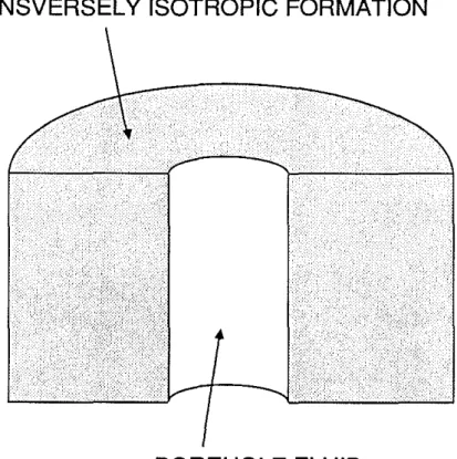
(24) Partial derivatives of phase velocity and related quantities like group velocity will be calculated for a fluid-filled borehole in a transversely isotropic formation (Figure 2). The model is appropriate for horizontally layered, sedimentary rocks through which a vertical borehole is drilled. Because the axis of symmetry for the transverse isotropy is aligned with the borehole, the elastic properties of the formation are characterized uniquely by only five elastic moduli, Cll, C13, C33, C44, and C66. (To derive the integrals

for this borehole model, matrix notation was used instead of tensor notation.) This model is also appropriate for an isotropic formation, for which the relations between the general elastic moduli and the Lame parameters are Cll

=

C33

=

A

+

2J.L, C13

=

A,

and C44

=

C66

=

J.L. The elastic modulus for the fluid is its incompressibility, Af> and is

related to the general elastic moduli via: Cll

=

C33

=

C13

=

Af with C44

=

C66

=

O.

The expressions for the displacements and strains, which are listed in Appendix A because they are quite lengthy, are substituted into the integrals in Eqs. (15, 16, 18, 19, and 20). The multiple integrals over volume and time are reduced to single integrals eliminating extensive computations. The procedure by which the reduction is performed and the resulting integrals, which will have the generic designation,

1,

are presented in Appendix B. The final integral associated with a perturbation in frequency is

j,t+T

dt

fv

dVPUiUi

=

TA1r1

5w ,

and with a perturbation in wavenumber, I,

rt+T r

51

J

t dt

J

v

dVOWejiCijklelk

=

olTAtrl

The final integral associated with a perturbation in either the fluid density (oPj) or formation density (oPs) is

[+T

dt

fv

dVOPUiUi = TAtr(oPj1Jp

+

ops1:

P) ,

(23)

and with a perturbation in either the fluid incompressibility (oAf) or any of the five elastic moduli for the formation (omi) is

j,

t+T

dt~ dVejiOCijkl€[k = TAtr(OAf1f'

+

2:,om;I:m5 i ) •

t V i=l

(

The simplified forms for the integrals can now be used to obtain the partial deriva-tives and other quantities. The general approach will be demonstrated by calculating the partial derivatives with respect to an elastic modulus of the formation. Substituting Eqs. (22) and (24) into Eq. (16) yields

(25) The wavenumber is related to the phase velocity, c, via: Ic = w, and at constant frequency 01 = -Ioc/c. (The lack of subscripts on the symbol for the phase velocity distinguishes it from the symbols for the elastic moduli.) The partial derivative of the phase velocity is

(26)

oc c 10m ;

__ = __

8 _

omi 21 1°/

The normalized form of this derivative,

m· Be m"jOmi

- ; omi

=?1

;0/

(27)

is dimensionless and is called the sensitivity. The formulas for the partial derivatives and sensitivities at constant frequency are listed in Table 1. At constant wavenumber, the expression, Ow

=

loc, is used to calculate the perturbation in phase velocity. The normalized derivatives are called partition coefficients, and these quantities with the associated partial derivatives are listed in Table 2. The sensitivities and partition coefficients can be interpreted as the percent change in phase velocity due to a one percent change in an elastic modulus or a density.

The simplified forms for the integrals are used to calculate the group velocity, U.

Eqs. (21) and (22) are substituted into Eq. (20) to yield

Ow 1 1°/

U

=

71

=

wlOW

(28)

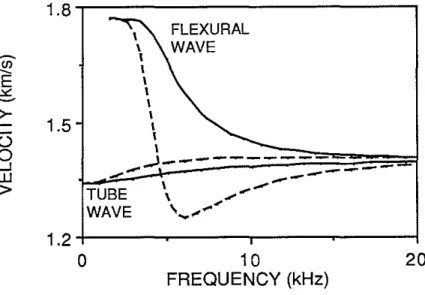
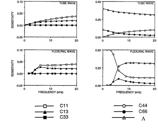
Sample calculations show how the equations, which were derived in this section, can be applied to guided waves. The integration over radius was performed numerically using a modified form of Gaussian quadrature and was terminated when the sum converged to four significant digits. The transversely isotropic formation was selected to be the Green River shale for which the physical properties are tabulated by Thomsen (1986). The phase and group velocities for the tube and flexural waves are shown in Figure 3, and the sensitivities at constant frequency in Figure 4.

(29)

s

=

Some simple additions can be used to check the accuracy of the sensitivities. Sum-ming the sensitivities associated with the elastic moduli for constant wavenumber gives:

Af

If'

s mi

I%m;

2w2 lOW

+

L

2w2 lOW

= (30)

The expression, T A1rw2lOW

/2,

is the time averaged kinetic energy, and the summation of the six terms within the brackets yields the time averaged elastic strain energy. Because these energies are equal, the sum,S, must be 1/2. Since each of the six terms in Eq. (29) is the fraction of the total elastic strain energy associated with a particular elastic modulus, the terms are frequently called partition coefficients. A similar check can be applied to the densities, and the sum must be -1/2. At constant frequency, the sensitivities must be multiplied by

U/c,

and the final sum must be 1/2for the elastic moduli and -1/2 for the densities. The computer programs, which were written to perform the calculations presented in this paper, almost always yield sums between 0.4999 and 0.5001, and higher accuracy could easily be obtained.

SLIGHTLY ANISOTROPIC FORMATIONS

The phase velocities of the guided waves are desired for a borehole model in which the elastic moduli of the layers are anisotropic and characterized by (Cijkl

+

8Cijkl). Because the displacements for this model are generally not calculable, Rayleigh's prin-ciple may be used. To apply this prinprin-ciple, moduli, Cijkl> for which displacements can be calculated are selected for each layer. The exact displacements and the perturbed moduli, 8Cijkl, are then substituted into Eq. (19) to obtain first order perturbation in phase velocity:

;"+7 dt

fv

dVeji8cijkleik 8c=

=---:;-;-'f;,'---2wl

;"+7

dt

fv

dVPUiUi in which the relation, 18c= 8w has been used.

(31)

An important step is extracting the moduli, Cijkl> from (Cijkl

+

8ci jkl). The ten-sor, Cijkl, must have the symmetry appropriate for either an isotropic or transversely isotropic medium because displacements can only be calculated for formations of these types. Moreover, Cijkl must be selected in a manner that makes 8Cijkl small to obtain the greatest range of validity for the perturbative method. Because

(32)

by Pythagoras' theorem, the best choice for theCijkloccurs when 118cijkzll2 in minimized (Backus, 1982). A convenient measure for the strength of the anisotropy is the ratio:

118cijklW

II

C_ijkzll2

which must be small compared to 1.

Eq. (31) has been applied to a fluid-filled borehole through a slightly anisotropic, infinite formation. The integral in the denominator is given in Eq. (21), and the integral in the numerator is listed in Appendix C because it is quite long.

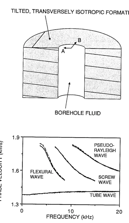
We created an anisotropic formation by tilting a transversely isotropic sandstone, for which the physical properties match the Taylor Sandstone listed in Thomsen (1986), ten degrees with respect to the borehole (Figure 5a). The strength ratio for the anisotropy is 0.023. The phase velocities for guided waves oriented perpendicular (A) and parallel (B) to strike are shown in Figure 5b. Because the tube and pseudo-Rayleigh waves have no azimuthal dependence, their dispersion curves are expected to be identical. The curves predicted by this perturbative method show that they are very close, and the slight difference is the inherent inaccuracy of the method. The largest errors occur for the tube wave at high frequencies and for the pseudo-Rayleigh wave at the cutoff frequency. The phase velocities for the flexural wave, for which the displacements vary as cos0, where 0 is the azimuthal angle, clearly show the effects of anisotropy, whereas those for the screw wave, for which the displacements vary as cos20, do not.

SUMMARY

The Lagrangian for a general borehole model with multiple, radial layers has been de-rived. Rayleigh's principle was used to calculate first order perturbations in wavenum-ber and frequency due to slight variations in the physical properties of the layers. The principle was similarly used to calculate perturbations in frequency due to perturba-tions in wavenumber.

These perturbative formulas are important because they are used to derive ex-pressions for partial derivatives which would be needed in an inversion for formation properties. These derivatives were developed for a fluid-filled borehole through an infinite, transversely isotropic formation, for which the axis of symmetry was aligned with the borehole. The derivatives are very accurate and only require one numerical integration, which is more stable than numerical differentiation. The perturbative for-mulas were also used to calculate the group velocity for this borehole model. Applying the formulas to this simple borehole model demonstrates the procedure by which they are be applied to more complicated models.

Rayleigh's principle was used to calculate the perturbation in phase velocity of a guided wave due to a slightly anisotropic formation. This perturbative formula was applied to a transversely isotropic formation, for which the axis of symmetry was tilted ten degrees with respect to the vertical borehole. The phase velocities for the tube

and pseudo-Rayleigh waves are nearly identical for different orientations of the waves relative to the formation. The velocity dispersion of the flexural wave depends upon its orientation whereas the dispersion of the screw wave appears not to be affected by the situations studied here.

ACKNOWLEDGEMENTS

This research was supported by the Full Waveform Acoustic Logging Consortium at M.LT.

REFERENCES

Backus, G .E., Reply: Limits of validity of first-order perturbation theory of quasi-p velocity in weakly anisotropic media, J. Geophys. Res., 87, 4641-4644, 1982. Burns, D.R., and Cheng, C.H., Inversion of borehole guided wave amplitudes for

for-mation shear wave attenuation values, J. Geophys. Res., 92, 12713-12725, 1987. Cheng, C.H., Toksoz, M.N., and Willis, M.E., Determination of in situ attenuation

from full waveform acoustic logs, J. Geophys. Res., 87, 5477-5484, 1982. Rayleigh, J.W.S., The Theory of Sound, v.l, Dover Publications, Inc., 1945.

Smith, M.L., and Dahlen, F.A., The azimuthal dependence of Love and Rayleigh wave propagation in a slightly anisotropic medium, J. Geophys. Res., 78, 3321-3333, 1973.

Stevens, J.L., and Day, S.M., Shear velocity logging in slow formations using the Stone-ley wave, Geophysics, 51, 137-147, 1986.

Thomsen, L., Weak elastic anisotropy, Geophysics, 51, 1954-1966, 1986.

Toksoz, M.N., Cheng, C.H., and Willis, M.E., Seismic waves in a borehole - a re-view, in Vertical Seismic Profiling, Part B: Advanced Concepts, Toksoz, M.N. and Stewart, R.R., eds., 256-275, Geophysical Press Limited, 1984.

Tongtaow, C., Wave propagation along a cylindrical borehole in a transversely isotropic formation, Ph.D. thesis, Colorado School of Mines, Golden, Colorado, 1982. Woodhouse, J.H., and Dahlen, F.A., The effect of a general aspherical perturbation on

64

Ellefsen and Cheng

APPENDIX A

Tongtaow (1982) derived the expressions for the displacements and strains associated with wave propagation in a borehole. His equations have been adapted for propagation along a fluid-filled borehole (Figure 2) and are listed here.

In the cylindrical coordinate system, r is the radial distance, z the axial distance, and

e

the azimuth. The axial wavenumber is I, the azimuthal order number n, and the radian frequency w. The functions for the radial dependence of the displacements in the fluid are

The displacements have the general form

ur(r,n,l,w)

=

Ur(r)ei(lz+nS+wt)

us(r,n,l,w)

=

Us(r)e- i1r/

Z

_ei(lz+nS+wt)

uz(r,n,l,w)

=

Uz(r)ei(lz+no+wt)

.

(A-1)

(

(

USer)

Uz(r)

and in the formation are

= Alml

[....!!:..-In(mlr)

+

In+l(mlr)]

mlr

A

l

--In(mlr)

r =

AlilIn(mlr)

(A-2) (

Ur(r)

=

-Az(l

+

ila')mz [-....!!:..-Kn(mzr)

+

Kn+l(mzr)]

+

mzr

Czn

Kn(kzr)

-r

Bz(

il

+

b')kz [- k:r Kn(kzr)

+

Kn+l(kzr)]

User)

=

-Az(l

+

ila'):::'Kn(mzr)

+

r

Czkz [-..:!:-J(n(kzr)

+

Kn+l(kzr)]

-kzr

Bz(il

+

b'):::'Kn(kzr)

r

Uz(r)

=

Az(il-

a'm~)Kn(mzr)

-

Bz(k~

- ilb')Kn(kzr)

(A-3)

(

The coefficients, Al , A

z,

B

z,

and C

z,

and the axial wavenumber are found by solving the period equation. Formulas for the wavenumbers, ml,

_{mz, kz,}

and

_kz,

and the coupling coefficients, a' and

b',

are given by Tongtaow (1982).

The strains have the general form:

(

I )

Err (r)e

i(lz+nS+wt)

eoo(r, n, I, w)

_{Eoo(r )ei(lz+nO+wt)}

ezz(r, n, l,w)

=

_{Ezz(r )ei(lz+nO+wt)}

ezo(r,n,l,w)

=

_Ezo(r)e-i

r;/2

_ei(lz+nO+wt)

ero(r,n,l,w)

=

Ero(r)ei(lz+nO+wt)

(

I )

=

Erz(r)e-i1r/2ei(lz+nO+wt)

erz r,n, ,W (A-4)

The functions for the radial dependence of the strains are

(A-5)

dUr(r)

dr

Ur(r)

+

nUo(r)

r

ilUz(r)

~

[ilUo(r) _ nU;(r)]

=

~

[ilUr(r)

+

dU;;r)]

=

~

[dUo(r) _ nUr(r)

+

Uo(r)]

2

dr

r

Eoo(r)

=

Ezz(r)

APPENDIX B

The integrals for a fluid-filled borehole through a transversely isotropic, infinite forma-tion (Figure 2) will be presented in this appendix.

The general procedure used in calculating these integrals is best demonstrated by considering a somewhat simpler integral:

(B - 1)

for which

Sj

=

Qj(r)ePj(-i~/2)ei(lz+ne+wt) . (B - 2)

The variable P_j is either 0 or 1. Only the real part of Sj is used as only the real parts of the complex displacements and strains are used. Using the relation Re Sj =

(Sj

+

S1)

/2,

the integral becomes

(B-3) after some algebra. Because the integral over time in the second part of this expression is zero, the multiple integral over time and volume (Eq. B-1) reduces to a single integral over radius.

This simplification is similarly applied to the integrals for the fluid-filled borehole using the displacements and strains listed in Appendix A. The generic designation for the integral over radius is

I.

The integral associated with a perturbation in frequency is

l+TdtlvdVpUiUi = TA7rl'OdrrP(lUrI2+lUeI2+lUzI2)

= TkrrI sw and with a perturbation in wavenumber

(B-4)

8ITA7r

faoo

drr{

CI3

[IE

rr

IliU

z

I

cos (arg

Err -

arg(

iU

z ))

+

C33 [IEzzlliUzl

cos (arg

Ezz -

arg(

iUz ))]

+

[

iUo

iUo

C44 41EzoIITI

cos(arg

Ezo -

arg(

T))

+

iUr

II (

iUr ]}

41ErziT

cos arg

_{Erz -}

arg(

T))

=

8ITA1rIo/ .

(B-5)

The integral associated with perturbations in either the fluid density

(p

f)

or the for-mation density

(Ps)

is

{HT {

J

t dt

J

v

dV8PUiUi

=

TA1r[faR drr8PJ

(IUr1

2

+

IUol2

+

IUz1

2)

+

l.co

drr8ps

(IUr1

2

+

IUol2

+

IUz

I

2)]

=

T A1r(8PJI;P

+

8PsI~P) ,

(B-6)

o

(B-7) in which R is the borehole radius. The integral associated with perturbations in the elastic moduli is

TA1r(f

drr

8>'f[IErr I

2

+

IEool2

+

IEzz l

2

+

21Err llEoo i

cos(arg

Err -

arg

_Eoo)

+

21Err ilEzz

icos(arg

Err - argEzz )

+

21EooIIEzzi cos(Eoo -

arg

Ezz )]

+

l.co

drr{

8C11 [IE

rr

12

+

IEoo l

2

+

21Err llEooi

cos(arg

Err -

arg

Eoo )]

+

8C13

[2lErrllEzzl

cos(argE

rr -

argEzz )

+

21EooIIEzzi

cos(Eoo -

arg

Ezz )]

+

8C33 [IEzz I

2

]

+

8C44 [41Ezo12

+

41 Erz1

2

]

+

8C66

[41 Ero1 2 - 41Err IIEoo

Icos(arg

Err -

arg

Eoo )

J})

5

= TA1r(8)'fI~>'

+

I:8m;l°m)

APPENDIX C

The integral for a fluid-filled borehole through a slightly anisotropic, infinite formation (Figure2) will be presented in this appendix. The integral uses the displacements and strains listed in Appendix A, and the procedure by which it is calculated is outlined in Appendix B. The final equation is

[HT [

J, dt Jv dVejilicijklelk

=

T

A'If

tOO

dr r{ licnlErrl2

+

liC1221Err

I

IEoo

Icos(arg

Err -

arg

Eoo)

+

'If

liC1321Err

IIEzzl cos(arg

Err -

arg

Ezz )

+

liC1441Err IIEzol

cos(arg

Err -

arg

Ezo

+

2')

+

'If

liClS41Err

I

IErz

Icos(arg

Err -

arg

Erz )

+

liC1641ErrilEroi

cos(arg

Err -

arg

Ero

+

2')

+

liC221Eool2

+

liC2321EooIIEzzi

cos(arg

Eoo -

arg

Ezz )

+

'If

liC2441EooIIEzoi

cos (arg

Eoo -

arg

Ezo

+

2')

+

liC2S41EooIIErzi

cos(arg

Eoo -

arg

Erz )

+

liC264lEoollErolcos(argEoo - argEro

+~)

+

liC33IEzz12

+

'If

liC3441Ezz IIEzo

Icos(arg

Ezz -

arg

Ezo

+

2')

+

liC3S41Ezz

I

IErz

I

cos(arg

Ezz -

arg

Erz )

+

liC3641EzzIIEroi

cos(arg

Ezz -

arg

Ero

+

~)

+

liC4441Ezol2

+

'If

liC4S81Ezo

I

IErz

Icos(arg

Ezo -

arg

Erz -

2')

+

liC4681EzoIIEroi

cos(arg

Ezo -

arg

Ero )

licss41Erz

l

2

+

IicS681ErzilEroI

cos (arg

Erz - argEro

+~)

Partial Derivative Partial Derivative

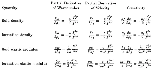
Quantity of Wavenumber of Velocity Sensitivity

01 W2 ]'P

8e

=

_we2~

]'P

fluid density

8pf

=T?

8pf 2 ] f!L.E.E... _e 8pf - j (we2 ]~ formation density 81 w 2 ]'P oe we2 ]'P Ps oe _ _ pswe!J:r

ops

= T]or

0ps

=

-T]or

e ops - 2 ]

01 I]'>' oe c ]0>' ],>,

fluid elastic modulus

OAf

= -'I?

OAf=21?

~..§.E...- ~~

e OAf - 21 ]

formation elastic modulus 01 1],m; oc c ]'m; rn-

OC

rn·jomi omi

=

-2]rr- omi

=

21]rr- -'----'~c omi - 21 ]

Table 1: Partial derivatives and sensitivities at constant frequency for guided waves in a fluid-filled borehole.

Partial Derivative Partial Derivative

Quantity of Wavenumber of Velocity Sensitivi ty

ow w]'P ]'P ]'P

fluid density

oPf

= -Z?w

oC e~

E.L

oe _ _ E.L~

oPf

= -'I]

w _{e oPf -} 2 ] w

formation density ow w]'P oe e ]'P Ps OC _ _ Ps ]{" 0ps

=

-Z]ZW ops

=

-2]ZW e ops - 2 ] W

ow 1]8>. OC e]8>. ~ oe A]8>.

fluid elastic modulus

OAf

=

2w]t OAf

=

2w z

]t

e OAf

=

2:z

]t

formation elastic modulus ow 1],m; oc e ]'m; mi OC mi l

omi

omi

=

2]ow omi

=

2w z ]ow

C

omi

=

2w z ]ow

Table 2: Partial derivatives and sensitivities at constant wavenumber for guided waves in a fluid-filled borehole.

A

Figure 1: General model of a borehole with many fluid (white) and solid (shaded) layers. The outermost layer actually extends to infinity in the radial direction.

TRANSVERSELY ISOTROPIC FORMATION

BOREHOLE FLUID

Figure 2: Model of a fluid-filled borehole through an infinite, transversely isotropic formation.

1.8 . . . - - - ,

~

()

o

....J UJ

>

1.5

-l---20

10

FREQUENCY (kHz)

1.2

-1---~--__._--~---i

o

Figure 3: Phase (solid line) and group (dotted line) velocities for tube and flexural waves. The borehole model is shown in Figure 2; the formation is the Green River shale.

FLEXURAL WAVE 0.25 0.50r---.,.Tn;UB"E,.,W"'A"'V~E 0.25 0.50",...,.---"F"LE"XTiUR"'A"L"W"'A"VE'" 20 TUBE WAVE 10 0.10 ~ 0.05 > >= ;; z w 0.00

"'

..(J,OS 0 0.10 20 10 FREQUENCY (kHz)

0.00L..L::~~

_o 20 10 FREQUENCY (kHz) -0.05+---~----__J o 0

-••

C11 C13 C33 - 0 - - CM • C66

ts.

A

Figure 4: Velocity sensitivities at constant frequency for the tube and flexural waves shown in Figure 3.

TILTED, TRANSVERSELY ISOTROPIC FORMATION

BOREHOLE FLUID

1.9

~

.!!2

"',

E

e.

>- I-<.)

9

1.6

LU SCREW

>

WAVE LU (J)

«

_{TUBE WAVE}

:::c

a..

1.3

0

10

20

FREQUENCY (kHz)

Figure 5: (a) Model of a vertical borehole through a transversely isotropic formation for which the axis of symmetry is tilted ten degrees with respect to the vertical. (b) Phase velocities of the guided waves. The solid and dotted lines correspond to orientations A and B, respectively (shown in part a).