Analytical model for a cylinder sinking into a thin film

Analytical Model for a Cylinder Sinking Into a

Thin Film

by

Kevin T. Chen

Submitted to the Department of Mechanical Engineering

in partial fulfillment of the requirements for the degree of

Bachelor of Science in Mechanical Engineering

at the

MASSACHUSETTS INSTITUTE OF TECHNOLOGY

June 2005

©

Massachusetts Institute of Technology 2005.

Author ... .

...

,;

n-.

,, ..

.--

-

A/r.

All rights reserved.

JepL.[ l-bIlUl l 131 IVliUnai'gllll. 11 111UzLIIL May 6, 2005 ( Certified by . ... .

..

Assistant Professor

Thesis Supervisor

Accepted

by...

Ernest G. Cravalho

Chairman of Undergraduate Thesis Committee

ARCHIVES MASSACHUSES INSTIUtr OF TECHNOLOGY JUN 0 8 2005

I.... LIBRARIES

...

.-.

~1..-..-

; .- l ' ns-r~

,

- .;

r .

. ...

Analytical Model for a Cylinder Sinking Into a Thin Film

by

Kevin T. Chen

Submitted to the Department of Mechanical Engineering

on May 6, 2005, in partial fulfillment of the requirements for the degree of

Bachelor of Science in Mechanical Engineering

Abstract

New technologies and techniques have enabled oil companies to access oil deposits by

drilling through the ground horizontally. These increased capabilites have improved drilling efficiencies, and have also reduced the effects that drilling has on the local environment. These boreholes can be enormously long, and it is often necessary to send a tethered robot into the hole in order to gather information. If these robots

remain stationary for too long, however, their tethering cables can become stuck in

the mud cake lining the walls. The recovery or replacement of these robots is time consuming and expensive, so it is desirable to understand how and why the cables

sink. In this analysis, the mud cake is modeled as a Newtonian fluid. The surface of the cable is approximated as being either parabolic or circular, and it is shown that the sinking is governed by exactly two dimensionless parameters in both cases.

Matlab is used to visualize the evolution of the fluid pressure distribution with time, as well as the time it takes for the cylinder to settle to 20 percent of the mud cake thickness.

Thesis Supervisor: Anette E. Hosoi

Acknowledgments

Special thanks to Peko Hosoi, Julio Guerrero, and Debra Blanchard for all of their thoughtful help.

Contents

1 Introduction 11

1.1 M otivation . . . 11 1.2 Scope of Analysis . . . 12

2 Derivation 15

2.1 General Case for Newtonian Fluid ... 15 2.2 Parabolic geometry ... ... 18 2.3 Circular geometry ... 20

3 Analysis 23

3.1 Parabolic Geometry ... 23 3.2 Circular Geometry ... 25

A List of symbols used 33

B Derivation of Fluid Velocity 35

C Matlab Code 37

C.1 Parabolic geometry ... 37 C.2 Circular geometry ... 40

List of Figures

1-1 Comparison of drilling strategies (taken from OTS Heavy Oil Science

Centre website) . . . 12

1-2 Example of an oil drill bit (taken from HowStuffWorks.com) .... . 13

1-3 Illustration of the sinking cylinder model ... . 14

3-1 Change in 1 with time ... . 24

3-2 Change in hb with time ... . 25

3-3 Change in

P

3-4 Change in hb with time ... . 30 3-5 Time to reach hb = 0.2 with respect to I 1 and H2 for an initial hb = 0.4 31

Chapter 1

Introduction

1.1 Motivation

Recent advances in oil drilling technology have enabled oil companies to bore horizon-tally through bedrock in order to access oil deposits. This reduces the environmental

impact of dlrilling, as it gives the drillers more flexibility in selecting their drilling

sites. With this added flexibility, oil deposits located directly below environmentally sensitive areas can be tapped without negative effects to the land above. In

addi-tion, multiple horizontal branches can be drilled from a single hole, which reduces the overall number of holes that must be drilled.

In order to drill such deep holes, oil companies must use specially designed hollow

drill bits. I)rilling mud is pumped through the drill string, and it flows out through holes in the drill bit. This mud lubricates the bit as it cuts through the bedrock, then carries sediment and debris from the drilling up to the surface. For horizontal drilling, the drill bit is attached to a steerable downhole motor, which allows operators to adjust the angle of the bit as it drills. Current technology enables drillers to change

the angle of a well up to 110 degrees within just a few hundred feet, and horizontal holes have been drilled to lengths of over 35,000 feet [4].

When drilling of the well has ceased, a remote-controlled robot is sent into the

hole on a steel cable tether to gather data about the well. These wells, however, are

Figure 1-1: Comparison of drilling strategies (taken from OTS Heavy Oil Science

Centre website)

the wells can be enormous (300-500 degrees F, and 20,000 psi). Although the pressure is naturally high due to hydrostatic pressure, drillers typically keep the mud-filled

holes artificially pressurized in order to prevent the walls from collapsing. Such high pressures force the mud to leach into the dirt covered walls of the well, forming a

thin, viscous mud cake layer between the mud and the bedrock. If left to settle, the robot's tether cable can sink into this layer of mud cake; after about 20 minutes, the cable is unrnovable. The cost of either recovering or replacing the robot is enormous, so gaining a thorough understanding about how the cylinder sinks is of great interest

to oil companies.

1.2 Scope of Analysis

The mud cake can be modeled as a Bingham fluid. In a Bingham fluid, the fluid does not shear until it reaches a certain yield stress, above which it behaves as a

Newtonian fluid. As a first-order approximation, this analysis models the problem as

/ ..

maps W

il-11100

an infinite cylinder sinking onto an infinite plane, with the mud cake approximated

as a thin film of Newtonian fluid. In this case, it is shown that the sinking of the cylinder is governed by exactly two dimensionless parameters, whether the surface of

the cylinder is approximated as parabolic or circular.

7Ox

Mud

dV

Figure 1-3: Illustration of the sinking cylinder model

° ' .. .. . .' ' . ' ' ' ','' . . . .. . . . . .. · . · ·· .. .. . . .. .· . . .. . -. . . ., .- ,. . . . .

.... ... ...

...

...

...

... ...

...

... . ... ...

.... ... ... M

_{... ...}

...

... ...

_...

... ...

_...

Chapter 2

Derivation

2.1 General Case for Newtonian Fluid

The steel cable typically has a diameter of about one inch, whereas the diameter

of the oil well is usually six to twelve inches. Because the diameter of the cable is

significantly smaller than that of the well, the curvature of the well can be neglected,

and the problem can be approximated as a cylinder sinking on a flat surface (see Figure 1.3).

Furthermore, because the thickness of the mud cake is very small (usually about a quarter of an inch), the lubrication approximation can be used. This implies that the fluid velocity is small in the vertical direction, and that the pressure is a function only of x (horizontal position) and t (time). In the first part of the analysis, the mud

cake is modeled as a Newtonian fluid.

Using the lubrication approximation and imposing the no-slip boundary condition at the bedrock (y = ) and at the cylinder (y = h), one can find an analytical expression for the velocity in the x-direction (see Appendix B),

u(xyt)

(5)

)(y

h(x,

where hb(t) represents the position of the bottom of the cylinder as a function of time, and A(x) represents the geometric shape of the cable. In this analysis, parabolic and circular profiles are examined.

Imposing a simple mass balance on a differential control volume under the sinking cylinder, one can derive the expression

Oh 1 .0 OP h3_{)= 0. (2.3)}

a-7 12/i x 9,x °

Because only the hb portion of the expression for h varies with time, Equation 2.3 is

rewritten as

Ah 1b 0 (09 h3 h = . (2.4)

Otl 12 Ox Ox

J

The aP term can be found by performing a force balance on the cylinder. Gravity pulls the cylinder downwards while the fluid pressure pushes the cylinder upwards, and

inertial effects can be ignored because the cylinder sinks very slowly. An expression

for this resistance caused by fluid pressure can be determined from the dot product of fluid stress tensor and the normal vector to the cylinder surface. The fluid stress

tensor for a thin film of a Newtonian fluid, rTij, is

TiJ

-

Pay

uO

X,?

~ -P

= -Oh 'I) 1 (2.5)

Ox}

1

The dot product of these two expressions then, is the force exerted on the fluid by the sinking cylinder. As the x-component of this force cancels due to symmetry,

the only component of interest is the vertical force,

R _ _

Oh

u1

ohy =oAA71+ (2.6)0

The overall force on the cylinder can be calculated by reversing the sign of

Equa-tion 2.6 to represent the vertical force exerted on the cylinder by the fluid, then integrating over the area of the cylinder in contact with the fluid. For a cylinder of unit length, the expression becomes

mg I h p I

hs[

+P

S,

W is 2 x Oz ~/ + (h)2

where m is the overall mass of the cable, W is the overall length of the cable, and g

is the gravitational constant. This can be rewritten as

__= 2 [ a - _ - h

+

W

2.j

2Ox Ox

In the above expression, xm represents the maximum value of x at which the surface of the cylinder is in contact with the mud cake. It is clear, then, that xm increases as

the cylinder sinks.

Using this vertical force balance (Equation 2.8) along with the differential mass conservation equation (Equation 2.4), the height of the cylinder as a function of time

can be found. In order to obtain an analytically solvable set of equations, we use a

collocation method. To do this, the pressure p can be approximated as a second-order polynomial, namely

p(x, t)

po(t) + pi(t)x + p

(t)x

.

(2.9)

Since the pressure must be horizontally symmetrical with respect to the cylinder, however, the term must equal zero, which yields the simpler expression:

Furthermiore, the value of the pressure, p, must approach the ambient pressure as the horizontal distance from the cylinder increases. If this ambient pressure is defined to be zero, then the pressure boundary condition that p = 0 when x = m can be

imposed. This produces an expression for Po in terms of xm:

P = -p2xm. (2.11)

Incorporating these constitutive relations for the pressure, the preceding equations

can then be solved by using a Euler time step. Also, this analysis focuses on a very

small area directly below the cylinder, so it is valid to evaluate this expression at a Gauss point of x = 0 to simplify the expression. Assuming some initial condition, the

following discretized version of Equation 2.4 can be used to solve for hb+l:

hn1- hn p(hn)pn 3

b b 2 b (2.12)

At 6p '

where h refers to the current height, and hn+l refers to the height after the next time step.

Using h + l as a new initial condition, one can then recalculate the value of p2,

which will yield the next value of hb. After repeated iterations, this process eventually

determines the overall change in hb with time.

2.2 Parabolic geometry

As a first approximation, the profile of the cylinder can be approximated as a parabola.

This means that the height of the cylinder, h(x, t), can be written as

h(x,

This, in turn, leads to the following expression for the force in the y-direction:

where xm can now be calculated as

Xm =

T-hb

(2.15)

k

Again, xm simply represents the maximum value of x at which the surface of the

cylinder is still in contact with the mud cake layer. Now, substituting this expression back into the y-direction force balance (Equation 2.14) and integrating, the force balance equation becomes:

mg _{= - k} 4 2 5 2 3 23

P2 + -khb mP2 - _XmP2 (2.16)

W 5 m 33m

The constitutive relations between Po, P2 (2.11) and the expression for xm (2.15)

can be used to eliminate Po and xm from the above equation, which leaves only P2

and hb as unknowns. Assuming some initial value for hb, the value of P2 then can be

found analytically.

It is also helpful to non-dimensionalize the above equations so that the resulting

data are scalable to a variety of different physical parameters. The relevant variables are scaled as follows:

y = T (2.17) 1 x = x (2.18) k hb = Thb (2.19) t = -t (2.20)

P

x/P

=

(2.21)

-2

km vgT

P2 = PW (45 m+ 3 Tk.

-Xm = V/Tk(1l-h). (2.24)

Once the value for P2 is known, the dimensionless mass balance relation,

hn+l - hn T2_k2

At 6 P2(hb) (2.25)

can be used to determine the change in hb with time.

2.3 Circular geometry

A more accurate expression for the profile of the cylinder surface is a circle.

means that the height of the cylinder above the bedrock must be written as

h(x, t) = hb + R- VR2_{- x.}2

This

(2.26)

Integrating the pressure across the lower surface of the cylinder, an expression for

the force exerted on the cylinder by the fluid can be found as

2j mx

[( 2 R2)(&) ) (

vR

Xm

=

R

_-

_(T-hb-

_-R)

_.

Again, this fluid pressure force can be balanced with the force of gravity and

combined with various constitutive relations to yield an expression for P2,

where

+ R) (R2 sin-1

It is helpful again to non-dimensionalize the governing equations in order to make them easily scalable. The parameters can be scaled with the same factors as in the

parabolic case, only using x = Rx in place of x = :. This yields an expression for

the non-dimensional P2 as

P2 = WR

+ 1)

-m

lFrn)

where 5m can be written as

-T2 - 2

-Jr = 2 -( -hb) + 2(I -hb).

Once P2 is found for a given hb, it can be plugged into the non-dimensional mass

balance,

hn+ l - hn T2

-t

6R

b)

At 6R2 b

to determine the evolution of hb with time.

-1 - 2(2 (2.31) (2.32) XM R ) -XM

R -

-

Chapter 3

Analysis

3.1 Parabolic Geometry

The non-dimensionalized equations for 2 and hb appear to be extremely complicated, but actually depend only on two dimensionless parameters,

HI k-m ,gT 11 1 ' -- and 112 = Tk. (3.1) (3.2)

As such, Equation 2.23 can be rewritten as

P2 =1

(

±45

2x

-1

n+l n i- 2

b~+ -b = 62(h)3.

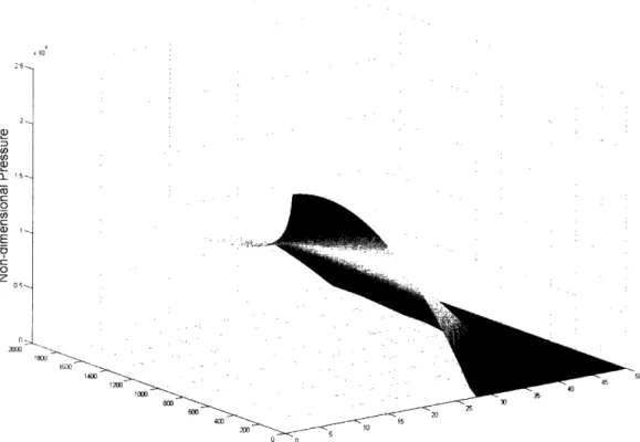
If typical physical parameters for the system are used, and the initial position of the cylinder is hb = 0.4, then the variation of non-dimensional pressure with x and

looks like: Viscosity = .001, k = 0.4 m-1, hinitial = 0.4 10 Cl) ID o) 0 V C a) E 0_. g 05% In-20 00- .-.. - I law.30 _11,00 a _ I . -',-'' -'.. 1200 1000 35 SOO ~0~~~~~~~~~~~~~~~~~~25 ~~~~400 C- ~ 15 10 0f 0 Non-dimensional Time*2000 Non-dimensional xm*1000

Figure 3-1: Change in

P

I2I5

~..

q . .

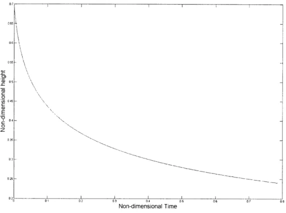
The change in the cylinder height with time looks like: 065 -to 05 _ t"-0 'j 045 E * 04 to 0 z 035 025 0 25 03 04 Non-dimensional Time 05 06 07 00

Figure 3-2: Change in hb with time

3.2 Circular Geometry

As with the parabolic geometry, the seemingly complicated expressions for P2 and hb

with circular geometry depend on just two dimensionless parameters. The parameters for the circular geometry are very similar to the parabolic parameters, and are defined

as

rgT

T

H12 - .

R

Using these H-groups in Equations 2.30, 2.31, and 2.32 respectively,

P2 = 1 [(I2hb + 1) (sin-(-m) - m

1-)

It is interesting to note that the mass balance equations for both geometries are identical (Equations 3.5 and 3.10), differing only in the definition of their respective

Hl-groups.

(3.7)

- 2]3

and

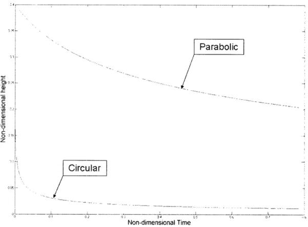
Assuming similar values to those in the parabolic case, but also that R = 0.5

inches, the variation in P with x and t looks like:

Parabolic

.... l*

Circular

... ...

Non-dimensional Time

Figure 3-3: Change in / with time

F) r-C .0 _(O %2 C a) E z 4

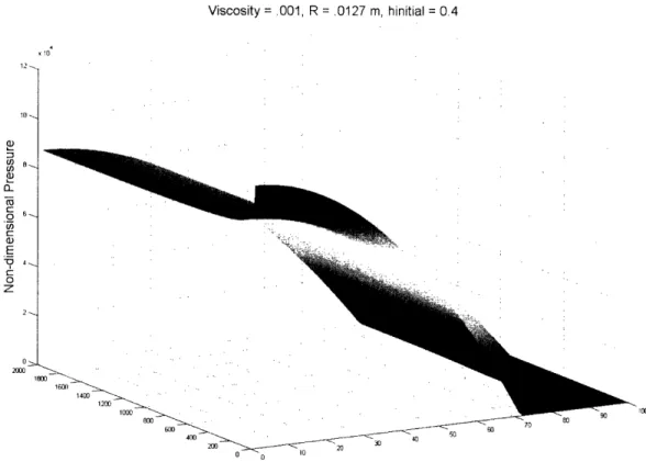
The variation of hb with t looks like: Viscosity = .001, R = .0127 m, hinitial = 0.4 1400 ₁₂₀₀ -. ~ ~~~~~~~~~~~~~~~~~~~ -1 ' Rnn - .. MA 6 4000 200 0 2 - 0 32 4 0 Non-dimensional Time*2000 70 Non-dimensional Position*100

Figure 3-4: Change in hb with time

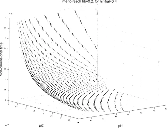
It is also interesting to examine the time it takes for the cylinder to sink to the

point where hb = 0.2, or 20 percent of the mud cake thickness. The following figure

displays these points for a range of HIll and 1-2 values.

12 '6-R1) 10 -o S ._ 0) E 4 0 z 2-. nO 2000 L 90 .. ... - . ,, . , - - .

Time to reach hb=0.2, for hinitial=0.4 o 2-.--35 Q; E -+.,25~ 0 To (42 2-E z 05 o 0 ; 87 2 5 _0 i 2220 28 ~~20 1 ,0t pi2 Ad pi1

Figure 3-5: Time to reach hb = 0.2 with respect to Ill and fI2 for an initial hb = 0.4

Appendix A

List of symbols used

Fy = vertical component of force exerted on cylinder g= gravitational constant

h = distance between ground and surface of cylinder

hb distance between ground and lowest point of cylinder surface

k = parabolic scaling constant, units of 1/meter

/ = fluid viscosity

p fluid pressure

po = pressure scaling constant, f(t), units of pressure

P2 = pressure scaling constant, f(t), units of pressure/square meters

1I = dimensionless parameter

R radius of cylinder

t= time

T = thickness of the mud cake layer

-ij = stress tensor

u = horizontal component of fluid velocity

v = vertical component of fluid velocity

W = length of the cylinder (z-direction)

x = horizontal position, where x = 0 corresponds to center axis of cylinder

x = maximum value of x at which cylinder surface is in contact with mud cake

Appendix B

Derivation of Fluid Velocity

The vertical distance between the cable and the bedrock is small compared to the horizontal span of the system, therefore the lubrication approximation can be used. This means that it is valid to assume that the pressure does not vary in the vertical direction,

,P =0, (B.1)

-=0

and that the vertical component of the fluid velocity is negligible,

v 0. (B.2)

With these assumptions, the relationship between pressure and velocity,

(

II ) (B.3)

can be integrated twice to yield the following expression:

1 9 y2+Ay+B. (B.4)

u 21p Ox(B4

A and B are integration constants that can be found using boundary conditions. These no-slip boundary conditions simply state that the fluid velocities at the bedrock

Ulh=O = 0, and

Ulh=h = O. (B.6)

Imposing these boundary conditions yields the following expression for the fluid

velocity:

u(x,

_hy).

2/t x] (B.7)

Appendix C

Matlab Code

C.1 Parabolic geometry

k = .4; %parabolic shape constant

T = .00635; %in m g = 9.81; mu = 0.001; in Pa-s :m = 3.98; %in kg %hb - T*hb Xx x/k Xp ~ p*mu/sqrt(T/g) Xp2 - p2*mu/k-2sqrt(T/g)

hn = hb;

deltat = .00001/sqrt(T/g); set time step amount

maxxm = round(1000*sqrt(T*k)); %maximum value of 1000*xm

for (i=1:2000) %i represents time step

hb = hn; xm = sqrt(T*k*(1-hb)); p2 = k*m*sqrt(g*T)/mu/(4/5*xm^5 + 2/3*T*k*hb*xm-3 - 2/3*xm^3); hn = TA2*k-2/6*p2*hb-3*deltat ₊ hb; hlist(i) = hn; p21ist(i) = p2; pOlist(i) = -p2 * xm-2;

for (j = :maxxm) %j represents x step

if (j/1000 <= xm) plist(i,j) = -p2*xm^2 + p2*(j/1000)^2; else plist(i,j)=O; end end

end

t = [O:deltat:deltat*2000-deltat]; nondimensional time

%t = [0:.00001:.01999]; %dimensional time x = [0:.001:.036]; figure(1); plot(t,hl:ist); xlabel('Non-dimensional Time'); ylabel('Non-dimensional height'); figure(2); plot (t,polist); xlabel('Non-dimensional Time'); ylabel('Non-dimensional p0'); figure(3); plot(t,p2list); xlabel('Non-dimensional Time'); ylabel('Non-dimensional p2'); figure(4); surf(plist); ylabel('Non-dimensional Time*2000'); xlabel('Non-dimensional xm*1000'); zlabel('Non-dimensional Pressure');

C.2 Circular geometry

%4/28/05

%Non-dimensionalized equations

%h = hb + R - sqrt(R-2-x-2)

%variable Gauss point

clear all;

R = .0127; %radius of cylinder, in m

T = .00635; %thickness of mud cake, in m

g = 9.81;

mu = 0.001; %viscosity, in Pa-s

m = 3.98; %mass of cylinder per unit length, in kg

%hb T*hb

%x R*x

%p p*mu/sqrt(T/g)

%p2 - p2*mu*R-2sqrt(T/g)

hb = 0.4; %set initial condition

hn = hb;

deltat = .000001/sqrt(T/g); set time step amount

W = 1; %unit length of cylinder

xg = 0; %Gauss point

maxxm = 100; %maximum value of 10000*xm

hb = hn; xm = 1/R*sqrt(R^2 - (T-T*hb-R)-2); p2 = m*sqrt(g*T)/2/mu/R/((T/R*hb+1)*(-xm/2*sqrt(1-xm-2)+1/2*asin(xm))-xm-3); hn = R/6/T*p2*((T/R*hb+1-sqrt(1-xg-2))-3 - 3*xg-2*(T/R*hb+1-sqrt(1-xg-2))-2/sqrt( xmlist(i) = xm; hlist(i) = hn; p21ist(i) = p2; pOlist(i) = -p2 * xm-2;

for (j = :maxxm) %j represents x step

if (j/100 <= xm)

plist(i,j) = pOlist(i) + p2*(j/100)Y2;

e:Lse

plist(i,j)=O;

end

end

end

t = [O:deltat:deltat*2000-deltat]; nondimensional time

figure(1);

plot (t hlist);

xlabel(' Non-dimensional Time');

ylabel ( Non-dimensional height');

figure(2);

plot (t,polist);

xlabel( Non-dimensional Time'); ylabel( Non-dimensional p0'); figure(3); plot(t p2list); xlabel('Non-dimensional Time'); ylabel('Non-dimensional p2_'); figure(4); surf(plist); ylabel('Non-dimensional Time*2000');

xlabel( 'Non-dimensional Position*100');

zlabel('Non-dimensional Pressure');

Bibliography

[1] I.S. Gradshteyn, I.M. Ryzhik, and Alan Jeffrey. Table of Integrals, Series, and

Products. Academic Press: 4th Edition, 1965.

[2] J. Happel and H. Bremer. Low Reynolds Number Hydrodynamics. Prentice-Hall, 1965.

[3] Ko Fei Liu and Chiang C. Mei. 1989. Slow spreading of a sheet of Bingham fluid

on an inclined plane. Journal of Fluid Mechanics, 207,505-529.

[4] Sara Pratt. A Fresh Angle on Oil Drilling. Geotimes, March 2004.