Anticipation nationwide risks to drinking water : predicting local scale contamination of community supply wells by gasoline additives

(1)

ANTICIPATING NATIONWIDE RISKS TO DRINKING WATER: PREDICTING LOCAL SCALE CONTAMINATION OF COMMUNITY SUPPLY WELLS BY GASOLINE ADDITIVES

by J. Samuel Arey

B.S., Public Policy and Environmental Science Indiana University, Bloomington

(1998)

Submitted to the Department of Civil and Environmental Engineering in partial fulfillment

of the requirements for the Degree of MASTER OF SCIENCE

in Civil and Environmental Engineering at the

atteMASSACHUSETTS INS-TjTTE

OF TECHNOLOGY

Massachusetts Institute of Technology

JUN 0 4 2001 June 2001

LIBRARIES

Signature of Author

Department ofg C 'and Environmental Engineering 25 May, 2001

Certified by

Philip M. Gschwend Professor of Civil and Environmental Engineering Thesis Supervisor

Accepted by_

Oral Buyukozturk Chairman, Departintal Committee of Graduate Studies

(2)

(3)

ANTICIPATING NATIONWIDE RISKS TO DRINKING WATER: PREDICTING LOCAL SCALE CONTAMINATION OF COMMUNITY SUPPLY WELLS BY GASOLINE ADDITIVES

by J. Samuel Arey

Submitted to the Department of Civil and Environmental Engineering on May 25, 2001 in partial fulfillment of the requirements for the Degree of Master of Science in Civil and Environmental Engineering

ABSTRACT

Only ten years after the increased addition of methyl-tert-butylether (MTBE) to U.S. gasolines, nationwide MTBE contamination of thousands of drinking water supply wells has been widely documented, reflecting enormous environmental and economic costs. Due to its abundance in gasoline, high aqueous solubility, and slow degradation rate in aquifers, MTBE has migrated in significant quantities from subsurface gasoline spills to a substantial number of community and private drinking water wells in a short period of time. For the purposes of this project, it was hypothesized that the tendency for gasoline additives to contaminate subsurface drinking water resources could be

accurately predicted a priori using a generalized transport model.

A screening method was developed to predict both the migration times of gasoline constituents from a leaking underground fuel tank (LUFF) to a community drinking water supply well and expected contaminant levels in the well. A review of literature revealed that U.S. municipal drinking water supplies are typically found in shallow sand and gravel aquifers. A subsurface transport model was parameterized based on the proximity of community supply wells to LUFTs (1000 in); probable characteristics of

sand and gravel aquifers; typical pumping rates of community supply wells (80 to 400 gal/min); and reasonable gasoline spill volumes from LUFTs (100 to 1000 gal). The transport model was tailored to individual solutes based on their estimated abundances in gasoline, gasoline-water partition coefficients (Kgw), and estimated organic matter-water partition coefficients (Kom).

Transport calculations were conducted for 17 polar and four nonpolar compounds currently proposed for or found in contemporary U.S. gasolines, including MTBE, ethanol, and methanol. Subsurface degradation processes were not considered. The transport model predicted MTBE concentrations of 40 to 500 ppb in municipal wells, which compared favorably with observed well concentrations at a significant proportion of sites in the U.S. The transport model therefore captured the order of magnitude of observed MTBE contamination of municipal wells without any use of adjustable or

(4)

Subsurface transport calculations of gasoline constituents required prior

knowledge or estimation of their gasoline-water partition coefficient and organic matter-water partition coefficients. In anticipation of the need to conduct transport calculations for novel or previously unstudied compounds, a review of methods for calculating or predicting solute partition coefficients in gasoline-water, organic matter-water, and octanol-water systems was conducted. Additionally, a new linear solvation energy relationship (LSER) was developed for estimating gasoline-water partition coefficients of organic compounds, having an estimated standard error of 0.22 log Kgw units.

Thesis Supervisor: Dr. Philip M. Gschwend

(5)

Acknowledgments

This research was supported by the Martin Family Society of Fellows for Sustainability, the Alliance for Global Sustainability, the Ralph M. Parsons Fellowship Foundation,

the Schoettler Scholarship Fund, and the Ford Scholarly Allowance.

Charles Harvey, Fatih Eltahir, Kris McNeill, John MacFarlane, Bill Green, Eleanor Kane, Ico san Martini, and the Gschwend laboratory research group at MIT all deserve my thanks

for their criticism and assistance regarding chemical and hydrogeologic modelling, statistical analysis, equipment and model support, and writing revisions. Additional thanks go to Al Leo (BioByte Corp.), Jim Landmeyer (USGS) Torsten Schmidt and Stephan Haderlein at the Swiss Federal Institute (ETH), Katsuya Kawamoto (Kanto Gakuin University), Toby Avery (Mobil-Exxon Corp.), Curt Stanley, Bruce Bauman, and Gerry Raabe at the American Petroleum Institute (API), and John Brophy and Jim Caldwell at the EPA for their contributions to my data gathering

efforts, legislative interpretations, model design and "real world" perspective.

I could not have completed this project without the continual support of my friends and parents. I am especially grateful for the guidance and endless enthusiasm provided by Phil Gschwend.

(6)

List of Tables

Table 2-1 A list of gasoline additives 20

Table 2-2 A list of other polar compounds found in retail gasolines 22

Table 3-1 Summary of water supply survey data for 6 randomly chosen U.S. communities 36

Table 3-2 Summary of model field transport parameters 36

Table 3-3 Summary of estimated transport model initial conditions and NAPL pool parameters 38

Table 4-1 Previous studies of the accuracy of UNIFAC predicted octanol-water partition coefficients 53

Table 4-2 Previous studies of the accuracy of MOD predicted partition coefficients 54

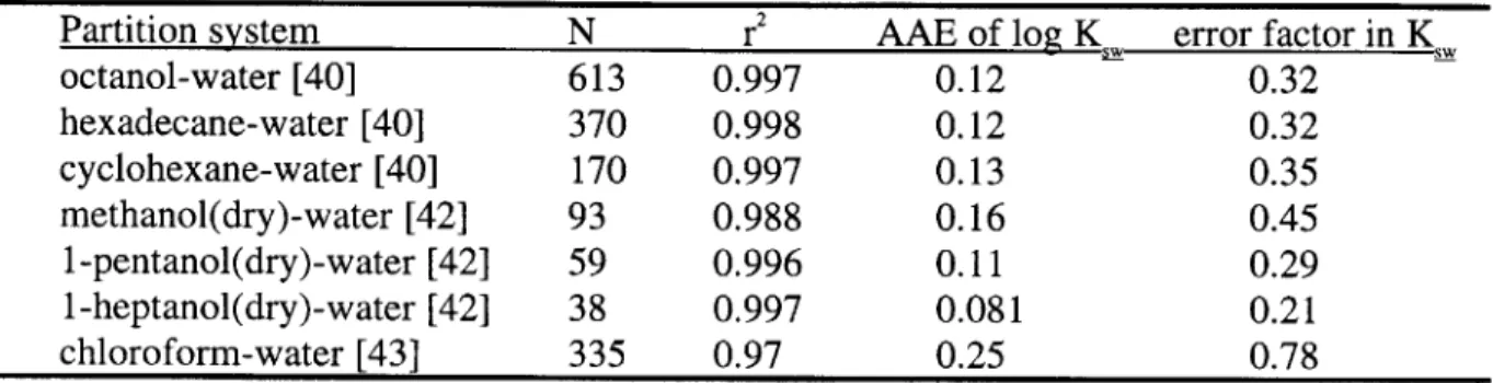
Table 4-3 Previous studies of the accuracy of LSER predicted partition coefficients 55 Table 4-4 Previous studies of the accuracy of GCS predicted partition coefficients 60

Table 5-1 Measured K. and K data at 25 "C 68

Table 5-2 Composition of the hypothetical gasoline mixture, "conventional syngas" 71

Table 5-3 Composition of "oxygenated syngas" 72

Table 5-4 Representative abundances of several compounds found in gasoline 73

Table 5-5 Syngas and aqueous activity coefficient values for gasoline solutes as calculated by UNIFAC

and AQUAFAC 74

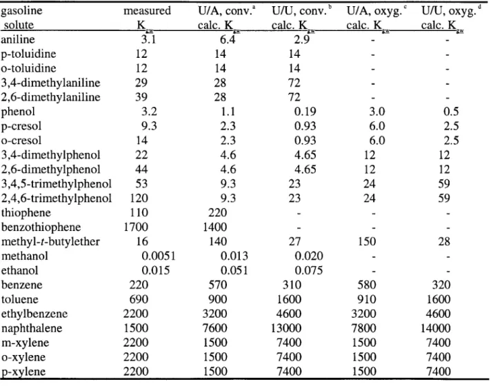
Table 5-6 Measured and calculated K, values for several compounds found in gasolines 75

Table 5-7 Estimated uncertainties of the LSER solvation parameter multipliers 80

Table 5-8 Measured or estimated K, values and solvation parameters used in the LSER regression 81

Table 5-9 Estimated standard error of isolated LSER multipliers 82

Table 5-10 Experimentally measured and ClogP calculated K0W's at 25 'C 84

Table 5-11 LFER-estimated Kom values for 21 compounds found in U.S. gasolines 86

Table 5-12 Subsurface transport parameters used for the standard case 87

Table 5-13 Physical property inputs used for the subsurface transport calculation 88

(10)

Table 5-15 Transport model results for the increased sediment organic matter content (0.5%) case 91 Table 5-16 Transport model results for the decreased well pumping rate (80 gal/min) case 93

(11)

List of Figures

Figure 3-1 Subsurface transport of compounds from a leaking underground storage tank 29

Figure 3-2 Streamline diagram of a well capture zone in a uniform flow field 33

Figure 3-3 Zone of contamination beneath the NAPL phase 37

Figure 5-1 LFER between Kgw and KW for different compound families 69

Figure 5-2 Partition coefficients between conventional syngas and water, calculated using UNIFAC for activity coefficients in both conventional syngas and water 76

Figure 5-3 Partition coefficients between conventional syngas and water, calculated using UNIFAC (for activity coefficients in syngas) and AQUAFAC (for activity coefficients in water) 77

Figure 5-4 Partition coefficients between oxygenated (10% MTBE) syngas and water, calculated using

UNIFAC for activity coefficients in both oxygenated syngas and water 78

Figure 5-5 Partition coefficients between oxygenated (10% MTBE) syngas and water, calculated using

UNIFAC (for activity coefficients in syngas) and AQUAFAC (for activity coefficients in water) 79

Figure 5-6 Round robin prediction test of the derived gasoline-water LSER using independent data 83

Figure 5-7 Measured vs ClogP predicted K. values for 23 gasoline solutes 85

Figure 5-8 Arrival time of solute front vs well water concentration: the standard case 90

Figure 5-9 Arrival time of solute front vs well water concentration: increased sediment organic matter 92

Figure 5-10 Arrival time of solute front vs well water concentration: decreased well pumping rate 94

(12)

(13)

Chapter 1

Introduction. Assessing the Impact of Fuel Additives on National

Drinking Water Resources: Development of a Transport Modeling Methodology

1-1. Motivation and purpose

Accumulated experience with environmental contamination has continually led western society to reconsider questions about anthropogenic compounds, including the following: (1) How much of the contaminant is released into the environment? (2) Once in the

environment, how does the contaminant transport and transform, thereby controlling exposures to humans and ecosystems? (3) When these exposures occur, what health effects will result? The answers to these questions generate the basis for estimating the social costs of

environmental contaminants of interest.

These inquiries are not all feasibly addressed for most chemicals. Question 1 is usually the easiest to answer. In the case of groundwater contamination by fuels, the characteristics of releases are directly related to the estimated number of leaking fuel storage tanks and spillage releases from automobiles during refuelling. Question 3 is probably the hardest to answer: health effects studies are expensive and frequently inconclusive, and usually give information about only certain types of toxicity effects.

Since toxicity and health effects of a contaminant are difficult to address, heavy scientific focus is frequently placed on question 2, the environmental behavior of a contaminant: how does the compound travel and react in the environment, thereby resulting in human and ecological exposures? When this critical issue is resolved, the level of need for aggressive health effects testing and envionmental monitoring can be established. For example, although gasoline is

composed of hundreds of compounds, toxicity testing and environmental monitoring is only relevant for the few components that may produce significant exposures in the environment.

This preliminary environmental assessment raises a more salient and useful point, however. The transport and reaction behavior of a chemical could be studied before it is introduced to society on a large scale. This pre-emptive modeling could avert future environmental and human health damage and properly focus nationwide contaminant characterization and health effects testing.

In other words, if the environmental transport and reaction behavior of compounds such as tetraethyllead (TEL) and methyl-tert-butylether (MTBE) had been studied before they were added to gasoline, the massive environmental, human health, and economic costs incurred by their use might have been avoided. Industrial lead use has increased ambient atmospheric lead concentrations by a factor of 300 [1], and the use of TEL in U.S. gasoline has been linked to child lead poisoning on a national scale [1]. MTBE use in gasolines has resulted in the closure of thousands of drinking water supplies in the U.S. over only a few years, thereby constituting enormous economic and environmental setbacks for society [2-8].

(14)

Literally thousands of compounds are used or imported at quantities greater than 1 million lbs per year in the U.S., but basic toxicity data exist for only 10% of these [9]. Over 70,000 synthetic chemicals are now commercially used in the U.S., and about 1000 new compounds are developed for industrial or commercial use every year [10]. In light of accelerating chemical production, the ability to a priori assess the environmental transport behaviors of proposed commercial compounds clearly has enormous potential benefits in terms

of future human health and ecological and economic cost avoidance. Specifically, the

development of a modeling tool to predict the exposure levels of future gasoline additives is an important need, based on past experience with TEL and MTBE.

The purpose of this study was therefore to address the following problem. Given a hypothetical newly proposed organic gasoline additive, can one: (1) predict the subsurface transport behavior and drinking water exposures that will result, on a nationwide scale; and (2) tailor these predictions to individual compounds based on physical property estimation methods? Iffeasible and accurate, such calculations would allow the threat offuture proposed gasoline additives to drinking water resources to be rapidly screened before these additives are used nationwide.

1-2. The "ensemble average" transport modeling approach

How does one go about developing a model to predict a nationwide subsurface contamination problem? General methodologies for the prediction of compound transport in site-specific hydrogeologic settings have been mapped extensively [11-14]. This foundation can be extended to assess the environmental impact of contamination at a multitude, or distribution, of sites.

Clearly, making specific environmental contamination predictions for every leaking underground fuel tank (LUFT) site in the U.S. is a cost-prohibitive evaluation of the potential environmental costs of using a newly proposed gasoline additive. If possible, the hydrogeology of these sites must instead be generalized to model an "ensemble average" of probable transport behaviors in various hydrogeologic settings. The ensemble methodology does not specifically predict contaminant behavior at any individual site, but it might predict the order of magnitude effects at many or most sites. In other words, I hope to predict the nationwide drinking water contamination consequences of specific gasoline additives by calculating the average behavior of many gasoline spills.

Fortunately, some common sense can be used to restrict the set of gasoline spills under consideration. Since the receptor of interest is drinking water, it is useful to consider only those

gasoline spills that are within reasonable vicinity of a community water supply well.

Additionally, as a first approximation, only LUFT sources of contamination will be considered. LUFTs are a considerable source of groundwater contamination by gasoline: over 330,000 confirmed releases from regulated LUFTs were reported to EPA between 1988 and 1998 [15].

Substantial data exist on both LUFT locations and their locations relative to community supply wells [16].

(15)

Restricting the ensemble approach to this subset of gasoline spills substantially focuses the scope of the transport problem. Investigation of the literature reveals that if only areas near community supply wells are considered, variability in the transport parameters of the sites is significantly reduced. In other words, under these assumptions, critical hydrogeologic

characteristics of the transport problem are somewhat generalizable. This is discussed in greater detail in Chapter 3.

The ensemble approach is intended as a screening tool for regulators concerned about what compounds should be put in gasoline. It is therefore not very useful for modeling

individual site contamination. A larger goal of this approach is to lay additional groundwork for the large scale modeling of contamination transport, such as that in urban airsheds, rivers, or lakes [17-20].

1-3. Physical property estimation methods

As stated previously, rapid and accurate estimation of physical properties is desirable in the context of a transport screening model for gasoline additives. The rationale for this is two-fold. First, the whole point of a screening method is that it provides a low-cost tool for quickly determining whether a particular societal activity is likely to cause substantial risks or costs. Generally, laboratory measurement of physical properties relevant to environmental transport requires time and money, whereas a modeling procedure is rapid and inexpensive. Second, the "ensemble" approach is proposed with the larger goal of applicability to many kinds of

chemicals in other commercial and industrial contexts.

The current "state of the science" for calculating phase partitioning in pertinent environmental media is therefore reviewed, including estimation methods of octanol-water partition coefficients, gasoline-water partition coefficients, and organic matter-water partition coefficients.

1-4. Outline of thesis work

Chapter 2 addresses the composition of contemporary gasoline and the U.S. regulatory guidelines that protect water supplies from contamination by gasoline components. Although gasoline includes several heteroatomic organic (and hence somewhat water-soluble) compounds, most of these chemicals are not considered in regulatory guidelines, nor are they tested for in drinking water supplies. A set of two dozen relevant compounds found in gasoline was selected to test the physical property estimation methods and the transport modeling approach.

In Chapter 3, the transport model is outlined and the basis of the ensemble approach is defended using hydrogeologic data. Transport model parameters were derived and an example calculation is shown.

Chapter 4 is an overview of physical property estimation methods of partition coefficients and some benchmarks describing their accuracy and robustness. This chapter

(16)

describes the current state of the science, but it may also give insight into the future of physical property calculation methods.

In Chapter 5, the transport method and some physical property estimation methods are applied to several of the heteroatomic organic compounds found in gasoline (from Chapter 2). This chapter thus provides practical examples of the subsurface transport screening model. Additionally, it serves as a preliminary assessment of the potential drinking water impacts of the current (known) formulation of gasoline.

Conclusions and recommendations for future research and policy needs are discussed in Chapter 6.

(17)

1-5. Citations

1. Misch, A., Assessing Environmental Health Risks, in State of the World, A Worldwatch Institute Report on Progress Toward a Sustainable Society, L. Brown, Editor. 1994, W W Norton and Co.: New York, NY. p. 119.

2. Squillace, P.J., J.F. Pankow, N.E. Korte, and J.S. Zogorski, Review of the environmental behavior and fate of methyl tert-butyl ether. Environmental Toxicology and Chemistry,

1997. 16(9): p. 1836-1844.

3. Allen, S., Gas additive debatedfrom Tahoe to Maine. The Boston Globe, March 1, 1999. p. Al, A8.

4. Giordano, A., MTBEfound in N.H. drinking water, report says. The Boston Globe, March 1, 1999. p. A8.

5. Lien, D., Minnesota ethanol industry eager to replace polluting gas additive. Saint Paul Pioneer Press, January 29, 2000.

6. Staff, California board wants to eliminate MTBE. United Press International, February 9, 2000.

7. Staff, Clinton may act on gas additive. Associated Press, February 23, 2000. 8. Staff, Senate panel approves MTBE ban. Associated Press, September 7, 2000. 9. Johnson, J., Chemical Testing: Chemical makers volunteer to conduct toxicity tests on

commonly used chemicals. Chemical & Engineering News, March 8, 1999. p. 9. 10. Miller, G.T., Living in the Environment. 1996, New York, NY: Wadsworth Publishing

Company. p. 18, 550.

11. Kitanidis, P.K., Prediction by the method of moments of transport in a heterogeneous formation. Journal of Hydrology, 1988. 102: p. 453-473.

12. Mackay, D.M., P.V. Roberts, and J.A. Cherry, Transport of organic contaminants in groundwater. Environmental Science & Technology, 1985. 19(5): p. 384-392.

13. Thierrin, J. and P.K. Kitanidis, Solute dilution at the Borden and Cape Cod groundwater tracer tests. Water Resources Research, 1994. 30(11): p. 2883-2890.

14. Charbeneau, R.J., in Groundwater Hydraulics and Pollutant Transport. 2000, Prentice Hall: Saddle River, NJ. p. 375-418.

15. Davis, M., J. Brophy, R. Hitzig, F. Kremer, M. Osinski, and J. Prah, Oxygenates in Water: Critical Information and Research Needs. 600/R-98/048, Office of Research and Development, U.S. Environmental Protection Agency, 1998. p. 7.

16. Johnson, R., J.F. Pankow, D. Bender, C. Price, and J.S. Zogorski, MTBE, To what extent will past releases contaminate community water supply wells? Environmental Science & Technology, 2000. 34(9): p. 2A-9A.

17. Mackay, D. and E. Webster, Linking emissions to prevailing concentrations -exposure on a local scale. Environmetrics, 1998. 9: p. 541-553.

18. MacFarlane, S. and D. Mackay, A fugacity-based screening model to assess

contamination and remediation of the subsurface containing non-aqueous phase liquids. Journal of Soil Contamination, 1998. 17(1): p. 17-46.

19. Mackay, D., A.D. Guardo, S. Paterson, G. Kicsi, and C.E. Cowan, Assessing the fate of new and existing chemicals: a five stage process. Environmental Toxicology and Chemistry, 1996. 15(9): p. 1618-1626.

20. Mackay, D., A.D. Guardo, S. Paterson, G. Kicsi, C.E. Cowan, and D.M. Kane, Assessment of chemical fate in the environment using evaluative, regional and

(18)

local-scale models: illustrative application to chlorobenzene and linear alkylbenzene sulfonates. Environmental Toxicology and Chemistry, 1996. 15(9): p. 1638-1648.

(19)

Chapter 2

Identification of Current Fuel Additives: The Chemical Structures and Abundances of Polar Compounds Found in Western Gasolines

2-1. Introduction

In an environmental context, fuels are conventionally viewed as a mixture of nonpolar hydrocarbons. A few small, aromatic hydrocarbon components, which are somewhat water-soluble and therefore mobile in aquifers, are considered possible groundwater contaminants, according to regulatory and academic literature. More recently, the oxygenate, methyl-tert-butylether (MTBE), has been discovered to widely contaminate municipal water supplies, from leaking gasoline underground storage tanks or spills [1]. Other potential oxygenates have also come under scrutiny as a result [2-4].

In reality, fuels contain a variety of organic compounds with heteroatom-containing (nitrogen, oxygen, or sulfur) substituents. These compounds are generally more polar than hydrocarbon components. As a result, they are more water-soluble and thus more likely to transport rapidly and in significant quantities to drinking water wells. Regulatory and wellhead protection literature neither mentions the presence of heteroatom-containing compounds nor considers them an important threat to groundwater. Consequently, neither municipalities nor regulators are encouraged to analyze community drinking water supplies for them.

The purposes of this chapter were to: (1) briefly discuss how contamination of municipal water supplies by fuel constituents and additives is treated in current regulatory and academic literature; (2) review a list of heteroatomic organic compounds which are either additives or refining byproducts currently found in gasoline; and (3) motivate the development of subsurface transport modeling efforts focused on heteroatomic organic compounds found in gasoline.

2-2. Currently evaluated compounds in fuels

In regulatory guides and associated literature for municipalities regarding water supply contamination, the EPA characterizes gasoline and diesel fuel as posing a contamination threat from either "hydrocarbons," "volatile organic compounds" (VOCs), or "oxygenates" [5-7]. Exactly what compounds do these phrases refer to?

EPA wellhead protection guide literature describes "hydrocarbons" as the following compounds [8]: benzene, toluene, ethylbenzene, xylenes, C substituted benzenes, and naphthalene. "Volatile organic compounds" are described in the Safe Drinking Water Act as

[9]: benzene, toluene, ethylbenzene, xylenes, and several other chlorinated compounds (by law, there are no chlorinated compounds in gasoline). Currently used "oxygenates" include MTBE and ethanol, although several other oxygen-containing compounds have been proposed as fuel additives in academic and EPA literature [6].

(20)

Thus, according to regulatory literature, only a few oxygenates and aromatic

hydrocarbons are considered potential threats to water supplies from leaking underground fuel tanks (LUFTs). Until recently [10, 11], studies which considered water contamination by fuel constituents other than hydrocarbons and oxygenates have generally focused on identifying parties reponsible for fuel-associated subsurface contamination [12, 13].

In federal regulatory code (CFR), rules on the specific chemical composition of fuel constituents and additives are unrestrictive. Fuel additives must be registered with the EPA, with information about their chemical composition or the precise process for their production

[14]. EPA approves fuel additive compositions without academic or public oversight, as patent privacy precludes the agency from sharing specific composition information with the public. The only other notable restriction on gasoline, diesel fuel, and fuel additive compositions is that they "contain no elements other than carbon, hydrogen, oxygen, nitrogen, and/or sulfur."

Additionally, they must contain less than 1.5 percent wt/wt oxygen and less than 1000 ppm sulfur (the sulfur limit is currently undergoing revision, however) [14]. In summary,

heteroatom-containing compounds in gasoline other than those specifically mentioned thus far (i.e., compounds other than MTBE, ethanol, benzene, toluene, ethylbenzene, xylenes,

propylbenzene, or naphthalene) are largely unregulated. Their potential impact on human health and the environment as related to fuel spills is entirely unstudied in the public record.

2-3. Gasoline additives (other than oxygenates)

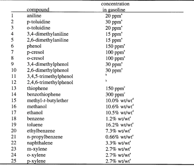
There are several specific compounds intentionally added to gasoline (Table 2-1). These compounds and mixtures improve engine performance, clean and lubricate engine valves, increase the octane number, improve emissions quality, preserve fuels during storage, and perform other functions [10, 15-19]. The concentrations of such compounds are in the 10 to 400 ppm range; lower than the abundances of typically studied gasoline constituents.

Table 2-1. A list of gasoline additives

N,N'-disalicylidene-1,2-diaminopropane [15] N

Use: chelating agent used to inactivate copper

Cfuel = 5 to 12 ppm OH HO polyisobutylated amines [16] Use: detergent/dispersant NH Cfuel = 100 to 250 ppm -H N n = 13 to 25

(21)

polyisobutylene mannich bases [16] Use: detergent/dispersant

CfUI = 100 to 250 ppm

aminated polypropylene oxides [16] Use: detergent carrier fluid

Cfuel= 100 to 250 ppm OH _r'\NH NHH NH HO n=8to 17 n =7 to 16 NH imidazolines [16] Use: detergent/dispersant Cf, = 20 to 60 ppm N,N'-disecbutyl-p-phenylenediamine (N,N'-dialkyl-p-phenylenediamines) [15] Use: antioxidant (preservative)

Cfuel = 5 to 20 ppm

2,4-dimethyl-6-tertbutylphenol [15] Use: antioxidant (preservative)

Cfuel = 5 to 100 ppm

butylated hydroxytoluene (BHT) [15] Use: antioxidant

Cfuel = 5 to 100 ppm

cerium (or other metal) naphthenates [17] Use: catalyst C = 25 to 50 ppm OH OH oas 0 0 )&3+ C>40 )&2 01,0-furfural [15] Use: dye/marker Cfuel = ? 0

(22)

diphenylamine [15] Use: dye/marker

Cfu = ?

QUO

N"0

2-4. Other polar compounds found in gasoline

In addition to gasoline additive compounds documented in the literature, there are several heteroatom-containing compounds which have been measured in U.S. and European gasolines (Table 2-2) [10-13, 18, 19]. These compounds may have originated in the crude oil as a result of natural processes, or they may have been formed or added during petroleum refining.

Table 2-2. A list of other polar compounds found in retail gasolines

benzotriazole [10]

C

fue 1-methylbenzotriazole [10] Cf = ? aniline [12, 10, 11, 13] Cfuel = 0.1 to 21 ppm [17] p-toluidine [12, 10, 13] Cfuel = 0.2 to 37 ppm [17] o-toluidine [12, 10, 11] C uel= 0.2 to 24 ppm [17] 3,4-dimethylaniline [10] C fuel= est. up to 16 ppm [10] 2,6-dimethylaniline [10] C u= est. up to 16 ppm [10] c N N N \ N ', NHZ NHZ NHI NHz NH2

(23)

OH phenol [12, 10, 11, 13] Cfuel = 0.8 to 170 ppm [10] p-cresol [12, Cfu = 0.3 to OH 10, 13] 120 ppm [10] o-cresol [12, 10, 13] Cfue = 1.5 to 130 ppm [10] 3,4-dimethylphenol [12, Cfuel = est. up to 40 ppm 2,6-dimethylphenol [11] 10, 11, 13] [10] OH Cfuel = est. up to 40 ppm [10] 3,4,5-trimethylphenol [12, 10] C fuel ? 2,4,6-trimethylphenol [12, 10] C fuel ? thiophene [18, 19] Cfuel = 18 to 178 ppm [19] benzothiophene [18, 19] Cfuel = 0 to 385 ppm [19] OH OH OH OH S

Q cT>

(24)

2-5. Discussion and conclusions

Like MTBE, most of the compounds shown in Tables 2-1 and 2-2 are fairly low

molecular weight and include one or more heteroatom-containing substituents. As a result, they are likely to be polar, somewhat water-soluble, and poorly retarded in aquifers. The high water solubility of these compounds will enhance their partitioning from fuel non-aqueous phase liquid (NAPL) to groundwater after a subsurface spill or leak. Thus, although many of the

heteroatomic organic compounds shown here are present in fuels at low concentrations, they may create high aqueous plume concentrations in aquifers as a result of their partitioning behavior.

Unlike MTBE, the compounds in Tables 2-1 and 2-2 are not generally tested for in municipal water supplies. Whether they are currently contaminating water supplies as

prevalently as MTBE is entirely unknown, since they may or may not have the same low "odor threshold" that originally brought MTBE to light as a potential drinking water safety threat [6]. It is important to note that the list of gasoline additives presented here is not necessarily

comprehensive. Due to trade privacy barriers, such a compilation would require rigorous experimental analysis of retail gasolines, which is beyond the scope of this study. However, published experimental investigations of gasoline components have generally considered the most light and highly polar compounds, that is, those most likely to solubilize in water [10-13].

The potential problem of water-soluble, highly mobile compounds transporting from fuel leaks to water supplies was the focus of quantitative modeling efforts discussed in subsequent chapters. The goal of these efforts was to propose a general modeling methodology by which proposed gasoline additives might be systematically pre-evaluated before use.

(25)

2-6. Citations

1. Johnson, R., J.F. Pankow, D. Bender, C. Price, and J.S. Zogorski, MTBE, To what extent will past releases contaminate community water supply wells? Environmental Science & Technology, 2000. 34(9): p. 2A-9A.

2. Huttenen, H., L.E. Wyness, and P. Kalliokoski, Identification of environmental hazards of gasoline oxygenate tert-amyl methylether (TAME). Chemosphere, 1997. 35: p.

1199-1214.

3. Wallington, T.J., J.M. Andino, A.R. Potts, S.J. Rudy, and W.O. Siegl, Atmospheric chemistry of automotive fuel additives: diisopropyl ether. Environmental Science & Technology, 1993. 27: p. 98-104.

4. Pacheco, M.A. and C.L. Marshall, Review of dimethyl carbonate (DMC) manufacture and its characteristics as a fuel additive. Energy & Fuels, 1997. 11: p. 2-29.

5. Gardner, S. and B. Moore, Case Studies in Wellhead Protection Area Delineation and Monitoring. 600/R-93/107, U.S. Environmental Protection Agency, 1993.

6. Davis, M., J. Brophy, R. Hitzig, F. Kremer, M. Osinski, and J. Prah, Oxygenates in Water: Critical Information and Research Needs. 600/R-98/048, Office of Research and Development, U.S. Environmental Protection Agency, 1998. p. 7,20,21.

7. Belk, T., J.J. Smith, and J. Trax, Wellhead Protection, a Guide for Small Communities. 625/R-93/002, U.S. Environmental Protection Agency, 1993. p. 13.

8. Hoffer, R., Guidelines for Delineation of Wellhead Protection Areas. 4405/93/001, U.S. Environmental Protection Agency, 1987. p. 2-16.

9. Phase I Rule of the Safe Drinking Water Act (SWDA). 1989, U.S. Code of Federal Regulations 42: Washington, DC.

10. Schmidt, T.C., P. Kleinert, C. Stengel, and S.B. Haderlein, Polarfuel constituents

-compound identification and equilibrium partitioning between non-aqueous phase liquids and water. 2001.

11. Potter, T., Analysis of petroleum-contaminated water by GC/FID with direct aqueous injection. Groundwater Monitoring and Remediation, 1996. 16(3): p. 157-162.

12. Kanai, H., V. Inouye, R. Goo, L. Yazawa, J. Maka, and C. Chun, Gas

chromatographic/mass spectrometric analysis of polar components in "weathered" gasoline/water matrix as an aid in identifying gasoline. Analytical Letters, 1991. 24: p.

115-128.

13. Youngless, T.L., J.T. Swansiger, D.A. Danner, and M. Greco, Mass spectral

characterization of petroleum dyes, tracers, and additives. Analytical Chemistry, 1985.

57: p. 1894-1902.

14. Sections 79.11, 79.21, 79.56(e). 1997, U.S. Code of Federal Regulations 40: Washington DC.

15. Owen, K., Gasoline and Diesel Fuel Additives. 1989: John Wiley & Sons.

16. Avery, T., Gasoline additive chemistry. Pers. comm., Exxon-Mobil Corp., (609) 224-2615, September 12, 1998.

17. Kirk-Othmer, Encyclopedia of Chemical Technology, 4th Edition. 1994, New York, NY: John Wiley & Sons.

18. Martin, P., F. McCarty, U. Ehrmann, L.D. Lima, N. Carvajal, and A. Rojas, Characterization and deposit-forming tendency of polar compounds in cracked

(26)

components of gasoline. Identification of phenols and aromatic sulfur compounds. Fuel Science and Technology International, 1994. 12(2): p. 267-280.

19. Quimby, B.D., V. Giarrocco, J.J. Sullivan, and K.A. McCleary, Fast analysis of oxygen and sulfur compounds in gasoline. Journal of High Resolution Chromatography, 1992.

(27)

Chapter 3

Fugacity and Transport Calculations:

Modeling the Partitioning and Mobility of Gasoline Additives From Leaking Underground Fuel Tanks (LUFTs)

3-1. Introduction and motivation

In this chapter, fugacity calculations and transport models were used together to describe how compounds in leaked or spilled gasoline: (1) partition from gasoline to water; (2) partition

from water to aquifer solids (i.e., sorb); and (3) advect and disperse downgradient with the ambient groundwater flow towards municipal wells or other important water resources. The goal of the modeling approach was to assess the likely non-degraded groundwater concentrations and migration times of fuel constituents at downgradient municipal supply wells. The ultimate objective was to develop a screening methodology for evaluating whether any compound added to gasoline might contaminate significant numbers of municipal wells on a national scale, assuming chemical degradation in the subsurface was negligible.

Fugacity-based modeling assumes chemical equilibrium between all phases of interest, and therefore assumes that time scales of physical phenomena (e.g., groundwater flow) are slow relative to time scales of physical chemistry phenomena (e.g., partitioning between various phases). Fugacity-based models have been used previously to assess compound transport in a

number of environmental contexts, including subsurface contamination [1, 2], air-shed modeling [3], and large scale and global transport [4-6].

An entire chapter was devoted to fugacity-driven transport modeling in order to emphasize that the threat of water supply contamination by fuel constituents is primarily

controlled by differences in compound physical properties (e.g., the aqueous activity coefficient of naphthalene vs. that of MTBE) rather than variability in hydrogeologic contexts (e.g., alluvial aquifers vs. karst aquifers). There were three primary reasons for this approach to evaluating the mobility of organic compounds in subsurface environments. First, regardless of the specific hydrogeology, compound properties will drastically influence compound mobility and transport.

Second, since the general problem of fuel leaks and spills is one that includes literally hundreds of thousands of subsurface systems, it makes little sense to evaluate the threats posed by gasoline components to groundwater with a "site-specific" modeling approach. For example, both MTBE and naphthalene are abundant fuel components exposed to the same set of hydrogeological conditions in fuel spills. However, MTBE, rather than naphthalene, has caused contamination on a large scale (thousands of sites) as a result of its unique physical properties [7, 8]. Finally, this investigation revealed that many hydrogeologic features in the vicinity of municipal water supply wells can be generalized. In other words, there is little variability in the transport parameters of these aquifers. In fact, the geological characteristics common to municipality water supply aquifers make them particularly vulnerable to contamination by highly water-soluble compounds such as those found in fuels (see Chapter 2). Accordingly, a highly relevant hydrogeologic context could be proposed to evaluate fuel additive transport from leaking underground fuel tank (LUFT) spills to municipal water wells.

(28)

Since the transport model is intended to screen the potential mobility of anthropogenic organic compounds, biological and chemical attenuation processes were not discussed here. The rates of degradation processes vary widely in different geochemical environments and depend highly on characteristics of local microbial communities and on properties of the compound of interest. As a result, most attenuation processes are difficult to predict even for site specific conditions without accompanying expensive and time-intensive experimental investigation. An important premise of this study is that environmental fugacity and transport behaviors of organic compounds can be more inexpensively and reliably predicted under a wide range of conditions than can environmental degradability. The purpose of this study was therefore to evaluate the potential threat that compounds may pose on the basis of their mobility in the environment. If individual compounds are shown to create significant risks based on their environmental transport behaviors, rigorous studies of their environmental transformation rates should be conducted.

The goals of this chapter were to: (1) describe fugacity calculations of the fuel-water partitioning and aquifer solid-water partitioning of organic compounds and discuss the validity of underlying assumptions; (2) describe a transport modeling approach which computes the advection and dispersion of a contaminant plume as it migrates through the subsurface and dilutes in a municipal supply well; and (3) combine the fugacity and transport calculations to develop a general subsurface transport screening model which reflects probable non-degraded contaminant concentrations at municipal wells downgradient of LUFTs. A "recipe" of complete and succinct instructions for conducting a detailed transport model calculation is given at the end of the Summary and Conclusions part of this chapter (section 3-8).

3-2. Fugacity computations offuel-water partitioning

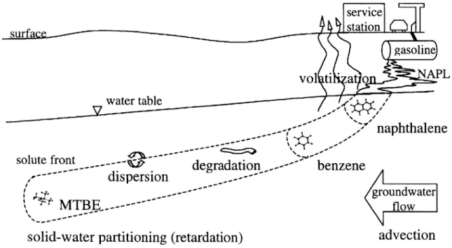
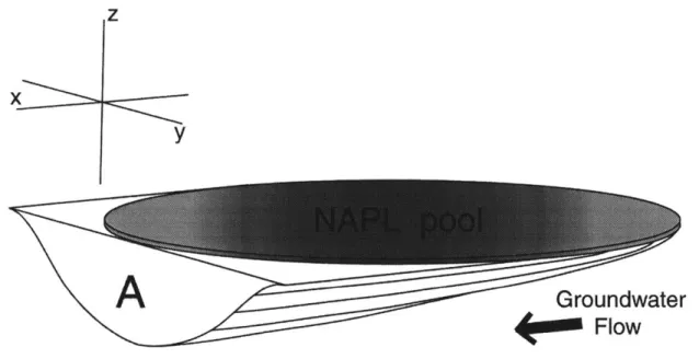
Consider a gasoline leak from an underground storage tank (Figure 3-1). As fuel

percolates through the vadose (unsaturated) zone, it pools on the water table. Since the aquifers of interest in this study are generally coarse grained and shallow (refer to section 3-4), gasoline transport through the vadose (unsaturated) zone was assumed to occur relatively quickly. Next,

individual compounds in the fuel mixture partition into the groundwater. The fuel-water inter-face was considered equilibrated with respect to chemical partitioning. In other words,

partitioning kinetics were assumed fast relative to groundwater flow and dispersion processes on the sub-grain scale. Finally, dissolved compounds are transported downgradient with the

groundwater flow and are subject to sorption to aquifer solids (retardation) en route. Sorption kinetics were also treated as fast relative to groundwater flow and sorption equilibrium was therefore assumed, as is discussed later (see section 3-3).

(29)

service station C)( surfa _I gasoline vol ti at o PL 7water _table I - - naphthalene

solute front. - _degradation_.-.---- _benzene

---- dispersion

--- ~~groundwater

MTB...---~ flow

solid-water partitioning (retardation)

advection

Figure 3-1. Subsurface transport of compounds from a leaking underground storage tank

The fuel-water partition coefficient, Kfw, describes the equilibrium concentrations of a compound between two adjacent phases:

KfW = C/Cw (3-1)

where Cf = concentration in fuel [mol L-'], and Cw = concentration in water [mol L'].

The partitioning of a solute is governed by the activity coefficients of the solute in different phases:

Kfw = (yV)/(yfV,) (3-2)

where Vf = molar volume of fuel phase (- 0.12 L mol~'),

Vw = molar volume of aqueous phase (- 0.018 L mol'),

yf= activity coefficient of solute in fuel [molfuel mol 11e-1], and y= activity coefficient of solute in water [molwatr mol ,i 1_].

An activity coefficient describes the nonideality of the solute in the phase of interest: the pure liquid phase of the solute itself is considered the "ideal" (reference) state, definitionally having

an activity coefficient value of unity. The molar volume of the aqueous phase is treated as equivalent to that of pure water. The molar volume of the fuel phase is formulated as the sum of fractional molar volumes of major fuel components (see section 5-3). The solute activity

(30)

AGS'. The excess free energy of solubilization represents the energetic cost of transferring the solute to a solution other than its pure liquid state (or reference state, in which AGe = 0):

y = exp(AGe/(RT)) (3-3)

If the solute activity coefficients, y, and y,, are known, K, can be used to approximate the solute concentration in the groundwater immediately adjacent to the fuel, given the fuel

concentration of the solute:

C, = C/Kf, (3-4)

The dissolved solute is now subject to the physical and chemical processes of groundwater transport as the solute plume migrates away from the fuel spill. Dispersion in the aquifer matrix will dilute and broaden the contaminant plume, and sorption to aquifer solids will retard its progress as it migrates (advects) with groundwater flow through the subsurface.

3-3. Fugacity modeling of sorption and retardation in the subsurface

The longitudinal velocity of the groundwater flow relative to the average rate of contaminant migration is defined as the retardation factor, R:

R = v water/vnnn (3-5)

For non-retarded transport, R = 1. Retardation occurs as a result of sorption of the contaminant to aquifer solids, thereby decreasing the contaminant's effective migration velocity through the subsurface. The retardation factor was formulated assuming that as a contaminant moves through the subsurface, a certain amount of it must spend time being sorbed to aquifer solids to maintain chemical equilibrium. The aqueous mass of the contaminant was considered here to be the portion that can migrate via groundwater flow at any given point in time (i.e., colloid-facilitated transport is ignored). The retardation factor can be expressed [9]:

R = 1 + Kdp,(1-$)/$ (3-6)

where Kd = sorption coefficient [L water / kg solid], PS = solids density [kg solid / L solid], and

= porosity [L water / L bulk aquifer material].

This derivation of the retardation factor (R) assumes that sorption equilibrium is achieved quickly relative to groundwater flow.

Organic compounds may sorb to multiple aquifer solid phases. However, studies have suggested that the organic matter in aquifer materials is the dominant sorbent for most nonpolar organic compounds [10-16]. These studies also suggest that sorption of nonpolar organic compounds to organic matter is approximately linear as a function of solute concentration

(31)

[13, 14], and that sorption behavior is similar for different sorbents [10-15]. Linear sorption isotherms suggest that the solute is partitioning between solvent phases (i.e., water and organic matter), rather than sticking to surfaces (adsorption). Adsorption is usually somewhat nonlinear, characterized by limited sorption sites with increased concentration or enhancement of sorption sites with increased concentration [17, 18]. As a modeling simplification, therefore, sorption was assumed here to occur dominantly to organic matter in the aquifer material:

Kd = fomKm (3-7)

where fom = aquifer solids mass fraction of natural organic matter, and

Km = organic-matter/water partition coefficient. The retardation factor may now be expressed:

R = 1 + f.KP, (1-$)/$ (3-8)

3-4. Advective - diffusive transport in the subsurface

The subsurface transport of a contaminant plume is governed by advection with ground-water (migration), retardation (sorption to solid phases), dispersion in three dimensions, and degradative processes. Representative field dispersivities, relevant hydrogeological

characteristics, and length scales to municipal wells were needed.

The hydrologic characterization of nationwide municipal well contamination by LUFTs can only be general. In the derivation of a subsurface transport model, the behavior of the groundwater contamination plume was treated as a longitudinally averaged slug with lateral and vertical Gaussian concentration distributions. This approach begs the question: why wasn't a more mathematically rigorous computational algorithm used, given the physical constraints of the system? A numerical calculation could easily have been devised to produce a three-dimensional plume distribution, with a precisely defined solute peak concentration and plume centroid. However, the level of overall hydrogeologic variability inherent in the thousands of subsurface sites considered here undermines the usefulness of such precision. Kitanidis reports that, especially when the regularity of hydrogeologic morphology is uncertain, the gaussian-like spreading of a plume does not necessarily reflect the extent of dilution of regions within the plume [19]. Clearly, the regularity of geological formations in the distribution of sites under consideration in this work (see section 3-5) is highly variable. The concentration distribution of the plume was therefore treated as a probabilistic, rather than deterministic, entity.

Additionally, variability in input parameters (see section 3-5) superimposed still more

uncertainty on model results. Therefore, it would have been an exercise in overmodeling to treat subsurface contaminant migration using a highly precise transport algorithm, thereby assuming a higher level of information than was actually available. Accordingly, the 3-dimensional

transport problem was solved by simply scaling the transport processes, as is described here. It is important to note that because of the uncertainty inherent in the modeling approach, the calculated municipal well contaminant concentrations must be interpreted as order-of-magnitude estimates. This is discussed further in Chapter 5.

(32)

The groundwater velocity (v), retardation (R) of the compound via sorption to aquifer solids, and transport distance (L,) can be used to estimate the time of arrival (tAr) _{of the front of a}

plug flow (i.e., non-dispersive) plume travelling from a LUST to a municipal well:

tAff, plug-fl = LXR/v (3-9)

In general, however, the time of arrival of the leading edge of the solute front is earlier than that suggested by plug-flow, depending on the extent of longitudinal dispersion of the plume. The longitudinal dispersion of the plume must therefore be characterized before the time of arrival of the solute front can be determined. The solute front is described (eqn 3-10) as the section of the plume that lies a distance , disp ahead of the plug flow front:

tArr, front = (Lx - Tx, disp)R/v (3-10)

where ax di,, = the square root of longitudinal variance of the dispersion-related plume spread. The spatial variance (a ) of the plume in any given direction i can be described as a function of the plume transport time (t) and dispersion coefficient (E) [20]:

dc /dt = 2(E/R) (3-11)

Assuming that dispersion is approximately Fickian (i.e., described as a random walk process), eqn 3-11 can be integrated from t = _{0 to the arrival time of the plume at the well (t}₌_{te,) with E,}

considered constant [20]:

G = 2(E/R)tArr (3-12)

It is well known that the dispersion coefficient, Ei, is not constant with respect to time in the field, contrary to eqn 3-11. In field studies, it has been shown that E, is proportional to the size of the plume [Welty, 1989 #21; Chrysikopoulos, 1992 #22; Kitanidis, 1988 #23]. The

dispersion coefficients used for modeling purposes here were empirically derived from field studies which assumed constant (time-averaged) Fickian dispersion [21]. This modeling approach is valid because the field studies from which the dispersion coefficient values were calculated involved transport over a spatial scale which was comparable to the transport scale considered here.

In this study, computing the extent of dispersion of the plume has practical value for three reasons. Longitudinal dispersion shortens the amount of time required for the contaminant to reach water supply wells (eqn 3-10). Additionally, longitudinal dispersion increases the spatial variance (or spread) of the plume, and therefore may decrease the average rate at which the contaminant enters the well. Finally, transverse and vertical dispersion determine whether the capture zone of the well is likely to draw the entire depth and breadth of the plume. We computed the probable extent of dispersion in all three dimensions, and addressed the consequences for transport accordingly.

(33)

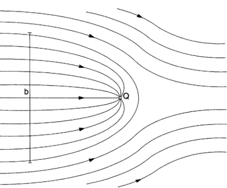
Consider the simple case of a municipal well drawing from the entire depth of a shallow aquifer in a relatively uniform flow field (Figure 3-2). The capture zone width of the well, b, is:

b = Qwl/(vh$) (3-13)

where Q,1 = well pumping rate [m 3/day],

v = ambient groundwater velocity [m/day], h = depth of the aquifer [m], and

$= aquifer solids porosity (unitless).

Figure 3-2. Streamline diagram of a well capture zone in a uniform flow field

The rate at which contaminant mass enters the well was calculated by multiplying the total mass of the contaminant in the plume (mo₀,1) by the velocity at which the contaminant is

transported (v/R), divided by the length of the plume at the well (roughly 2

x fina):

dm/dt, = m v/(2a R) (3-14

It is important to note that eqn 3-14 is a poor approximation for the contaminant mass flux into the well if the plume is very long as a result of leaching slowly out of the gasoline spill. In this case, the contaminant mass flux is approximated using the "steady state" transport solution described in section 7 of this chapter (eqns 3-39 and 3-40). The concentration of the compound in the water supply (Cweii) was determined by the rate at which mass of the compound enters a municipal well, divided by the pumping rate of the well (Qweii):

C11 = (dm/dtint we)/Qweii (3-15

)

(34)

3-5. Realistic field transport parameters

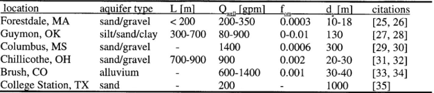
In order to make realistic calculations of contaminants transporting from LUFTs to community supply wells, reasonable field transport parameters were estimated. The choice of each transport parameter value is discussed in detail, based on literature review and a survey of six selected communities in the U.S (Table 3-1). The survey results included too few

communities to be very useful as an independent data set and are therefore shown mostly for validation of transport parameter estimates. The field parameters values chosen for the transport model are shown in Table 3-2.

Aquifer characteristics. A brief review of relevant literature demonstrated that municipal and domestic water supply wells are typically (purposefully) located in aquifers with high

hydraulic conductivities (10- to 102 cm/s) and porosities (0.10 to 0.50) [22-24]. In the U.S., the significant majority of water supply wells are drilled in unconsolidated deposits composed of glacial outwash sand/gravel or sedimentary/aeolian sand/silt deposits [22, 23]. To a lesser extent, fractured formation aquifers such as karst or fractured basalt are also exploited [22, 23]. Based on survey data (Table 3-1), we additionally hypothesized that the aquifers in which municipal wells are located generally have low organic carbon levels, with a solids organic matter fraction typically ranging from 0 to 0.005. For modeling purposes, we considered a sand and gravel unconsolidated aquifer with a saturated thickness of about 15 meters (50 feet) and solids organic matter fraction (f.) of 0.001.

Longitudinal groundwater velocity, v, determines the rate of subsurface transport of the contaminant. A review of field studies gives data for ambient groundwater velocities in several sand and gravel aquifers (n = 16) in the U.S. and Europe [21]:

range: v = 0.0003 to 31 [m/day]

median: v = 0.75 [m/day]

mean: v = 4.9 [m/day]

The longitudinal groundwater velocity was therefore assumed to be a constant value of approximately 1 meter per day in a uniform flow field. As shown by the data given above, this is a representative value for unconsolidated materials with high hydraulic conductivities. It is important to recognize that ambient groundwater velocity is a critical transport parameter which is highly variable between sites and regions, and results must be interpreted accordingly.

Distance to municipal wells, LX, sets the physical scale of the transport problem. In a recent nationwide survey of about 26,000 community water supply wells in 31 states, 35 percent

of municipal drinking water wells were found to be within 1,000 meters of at least one reported leaking underground gasoline tank [7]. Therefore, a representative LUFT to well distance of about 1,000 meters was assumed.

Dispersion coefficients EX, E,, and EZ represent the scale-dependent tendency for a plume to spread and dilute in the longitudinal (x), transverse (y), and vertical (z) directions. The dispersion coefficients are equivalent to the longitudinal (a), transverse (a ), and vertical (a) dispersivities multiplied by the longitudinal component of groundwater velocity, v [20]:

(35)

Ei = va, [m 2_/day]

Dispersivity, a,, reflects the tendency of a solute plume to dilute and spread during flow through a porous media. In the field, observed dispersivities are determined by the size of the flow regime, since geologic heterogeneities in the aquifer occur on multiple scales [20].

Representative field values of dispersivity in sand and gravel aquifers were obtained from data in a review by Gelhar et al., based on experimental transport distances of 500 to 1,500 meters [21]:

dispersivity observed in field [21]

dispersivity range average median n

ax [m] 7.6 to 234 50 20 7

ay [m] 1 to 4.2 3 4 3

a [m] 0.31 0.3 0.3 1

For comparison, according to the U.S. Environmental Protection Agency Composite Landfill Model (EPACML), typical subsurface dispersivities for a transport distance of 1000 m would be assigned the following probabilities in a stochastic simulation [20]:

dispersivity by probability

dispersivity p = 0.1 p = 0.6 p = 0.3

ax [m] 0.078 to 0.78 0.78 to 7.8 0.78 to 78

ay [m] 0.010 to 0.10 0.10 to 1.0 0.10 to 10

a, [im] 0.00049 to 0.0049 0.0049 to 0.049 0.0049 to 0.49

The following dispersivity values were considered representative for modeling purposes here:

a=10m a = I m a = 0.1m

Well Pumping Rate, Qwei, can range widely, depending on the needs of the community and the specific hydrologic setting. A survey of several communities suggested a municipal well pumping rate range of 435 to 7620 m3/day (80 to 1400 gal/min; Table 3-1). A higher pumping rate increases the likelihood that the capture zone will contain an entire contaminant plume, but it also lowers the effective concentration of the contaminant by diluting it with a greater volume of ambient groundwater. A pumping rate value of 2180 m3_{/day (400 gal/min) was thought to be}

reasonable for screening model purposes.

Table 3-1 shows a brief summary of data taken in the field survey. Fuel storage tank distances to community water supply wells (L) were estimated based on known well and service

station locations. In a few cases this data was not retrieved. Typical or average well pumping rates