Application of statistical learning theory to plankton image analysis

Application of St at ist ical Learning Theory to

Plankton Image Analysis

by

Qiao

Hu

B. S., University of Science and Technology of China(1990)

M.S., University of Science and Technology of China(1993)

Submitted to the Joint Program in Applied Ocean Science and

Engineering

in partial fulfillment of the requirements for the degree of

Doctor of Philosophy

at the

MASSACHUSETTS INSTITUTE OF TECHNOLOGY

and the

WOODS HOLE oCEANOGR~PHIC INSTITUTION

June 2006

@woods Hole Oceanographic Institution 2006. All rights reserved*

Thr lvthcr gmnn

o

RB

pemtrs(~3 to r~groducc to

fig'"'5 p f i " ~ ! ~ p ! i i ~ c ~ a j qfcst:;;iic ;opiL:t

e!

:a

eais ilocc:m

n!

whda

cr

In _{in arfy} ~ g j b - .m... ,.- ...

r cl:,da!g.&

. . .

Author

Joint Program in Applied Ocean Science and Engineering

-

C

April

25, 2006

. . .

. . .

. . .

Certified

by.

.

-

.

,

'.

Cabell S. Davis

Senior Scientist, WHOI

Thesis Supervisor

. . .

Certified by.

...

A.

Hanumant Singh

//

//

~s

at

soci

e

Scientist, WHOI

/

Thesis Supervisor

-

Accepted by . . .

Ed-;-

. . .

Henrik Schmidt

Chairman, Joint C o m m i t t w r Applied Ocean Science and

Engineering

. . .

. . .

. . . .

-

. . .

Accepted by

.#.

.,.

,

Lallit Anand

Chairman, Commit tee on Graduate Student

,

Department of

Mechanical Engineering

Application of Statistical Learning Theory to Plankton

Image Analysis

by

Qiao Hu

Submitted to the Joint Program in Applied Ocean Science and Engineering on April 25, 2006, in partial fulfillment of the

requirements for the degree of Doctor of Philosophy

Abstract

A fundanlental problem in lirnnology and oceanography is the inability to quickly ident,ify and map distributions of plankton. This thesis addresses the problem by applying st at ist ical niachine learning to video images collected by an optical sam- pler, the Video Plankton Recorder (VPR). The research is focused on development of a real-time automatic plankton recognition system to estimate plankton abun- dance. The system includes four major components: pattern reprc!sentation/feature measurement, feature extr action/select ion, classification, and abundance estimation. After an extensive study on a traditional learning vector quantization

(LVQ)

neural network (NN) classifier built on shape-based features and different pattern representation methods,

I

developed a classification system combined rnulti-scale co- occurrence rnatrices feature with support vector machine classifier. This new method ontperfor~ns the traditional shape-based-NN classifier method by 12% in classification accuracy. Subsequent plankton abundance estimates are improved in the regions of low relative abu~idamce by more than 50%.

Both the NN and SVM classifiers have no rejection metrics. In this thesis, two rejection rnetrics were developed. One was based on the Euclidean distance in the feature space for NN classifier. The other used dual classifier (NN and

SVM)

voting as output. Using the dual-classification method alone yields almost as good abundance estimation as human labeling on a test-bed of real world data. However, the distance rejection metric for NN classifier might be more useful when the training samples are not "good" ie, representative of the field data.

In sumrrlary, this thesis advances the current state-of-the-art plankton recogni- t'ion system by demonstrating multi-scale texture-based features are more suitable for classifying field-collected images. The system was verified on a very large real- world dataset in systematic way for the first time. The accomplishments include developing a multi-scale occurrerlce matrices and support vector niachine system, a dual-c1assific:ation system, automatic correction in abundance estimation, and ability to get accurate abundance estimation from real-time automatic classification. The

met,liods developed are generic and are likely to work on range of other image classi- fication applications.

Thesis Supervisor: Cabell S. Da.vis Title: Senior Scientist, WHOI Thesis Supervisor: Hanumant Singh Title: Associate Scientist, WHOI

Acknowledgments

First of all, I would like to thank my co-advisors, Cabell Davis and Hanumant Singh. They stand on my side with only occasional doubts. Even when

I

seemed have no way out. Cabell Davis was always there when

I

needed his guidance. His enthusiasm and "hands-on" approaches to science, both in the lab and during cruises, have been an inspiration to me. He is a great scientist and a good mentor. Hanumant Singh kept me on the track. He provided me the opportunity to share my work with fellow students. He is a really expert on underwater imaging.

I would like to thank the rest of my committee members, Jerome Milgram and George Barbastathis for their suggestions and useful criticism. I would like thank Carin Ashjian for serving as chair of my defense.

This work was supported by National Science Foundation Grants OCE-9820099 and Woods Hole Oceanographic Institution academic program.

I

would like thank Marine Ecology Progress Series for publishing my thesis Chapter 5 and 6 and giving me permission to include them in my thesis. Thanks to editors to make these two chapters more readable.

I would like thank everyone in the Video Plankton Recorder group. Cabell Davis, Scott Gallager, Carin Ashjian, Xiaoou Tang, Philip Alatalo, Andrew Girard and all the others collected the images I used in my thesis. Cabell Davis and Philip Alatalo taught me how to classify these images manually.

I would like thank everyone in Seabed AUV group. Hanumant Singh, Oscar Pizarro, Ryan Eustice, Christopher Roman, Michael Jakuba and Anna Michel gave me lots of comments and suggestions on my thesis work.

I ~vould like thank everyone at WHO1 Academic programs office. John Farrington, Judith McDowell, Julia Westerwater, Marsha Gomes and Stacey Brudno Drange made my long journey so wonderful and enjoyable.

I would like thank everyone who are kind enough to read my thesis draft. Judith Fenwick, Colleen Petrik, Gareth Lawson and Sanjay Tiwari read part or whole thesis.

Wenyu IJuo and Jinshan Xu, Zao Xu and Gareth Lawson.

I

had such a memorable time with them.

Last but not least,

I

would like thank my family. My wife Xingwen Li and my daughter Daisy Xuyuan Hu make such a warmth home for me. Their love, constant support and confidence gave me the great strength to break through all the difficulties. I thank my parents and my sisters for their understanding and patience.

Contents

1 Introduction 25

. . .

1.1 Motivation 26

. . .

1.2 Statistical pattern recognition 26

. . .

1.2.1 Features 27

. . .

1.2.2 Statistical learning theory 29

. . .

1.3 An overview of related work 30

. . .

1.4 Data 32

. . .

1.5 Thesis overview 33 2 Data Acquisition 39

. . .

2.1 Water column plankton samplers 39

. . .

2.2 Video Plankton Recorder 42

. . .

2.3 Focus Detection 44

. . .

2.3.1 Objective 44

. . .

2.3.2 Method 46

. . .

2.3.3 Algorithms 47

. . .

2.3.4 Result 48

. . .

2.4 Conclusion 52

3 Classification Method: Analysis and Assessment 53

. . .

3.1 System overview 54

. . .

3.1.1 Artificial Neural Networks 54

3.1.3 Principal component analysis

. . .

. . .

3.1.4 Feature extraction

3.1.5 Classification performance estimation

. . .

3.2 Assessment Result

. . .

3.2.1 Classifier complexity vs

.

classifier performance

. . .

3.2.2 Feature length versus classification performance

. . .

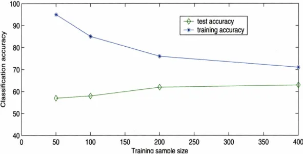
3.2.3 Learning curve - numbers of training samples versus classifier

. . .

performance

3.2.4 Initial neuron position versus presentation order of training

. . .

samples

3.2.5 Training samples effect

. . .

3.2.6 Classification stability

. . .

3.3 Two-pass classification system

. . .

3.3.1 Decision rules

. . .

. . .

3.3.2 Implementation

. . .

3.3.3 Results 3.3.4 Discussion

. . .

3.4 Statistical correction method

. . .

3.4.1 Method

. . .

. . .

3.4.2 Result

3.5 Distance rejection metric for LVQ-NN classifier

. . .

3.5.1 Distance rejection system

. . .

3.5.2 Result and discussion

. . .

. . .

3.6 Conclusion

4 Pattern Represent at ion/Feat ure Measurement 85

4.1 Pattern representation methods

. . .

86

4.1.1 Shape-based methods

. . .

86

4.1.2 Texture-based met hods

. . .

90

. . .

4.2 Feature extraction and classification 97

. . .

4.3 Results and discussion 100

. . .

4.3.1 High order moment invariants 103

4.3.2 Radial Fourier descriptors vs

.

complex Fourier descriptors

.

. 105

. . .

4.3.3 Co-occurrence matrices 107

. . .

4.3.4 Edge frequency 110

. . .

4.3.5 Runlength 111

. . .

4.3.6 Pattern spectrum 112

. . .

4.3.7 Wavelet transform 112

. . .

4.4 Conclusion 114

5 Co-Occurrence Matrices and Support Vector Machine 115

. . .

5.1 Co-Occurrence Matrices 116

. . .

5.2 Support Vector Machines 116

. . .

5.3 Feature Extraction and Classification 118

. . .

5.4 Classification results 119

. . .

5.5 Conclusion 126

6 Dual classification system and accurate plankton abundance estima-

t ion 129

. . .

6.1 Dual classification system description 130

. . .

6.1.1 Pattern representations 130

. . .

6.1.2 Feature extraction 132

. . .

6.1.3 Classifiers 133

. . .

6.1.4 Dual classification system 134

6.1.5 Classification performance evaluation and abundance correction 136

. . .

6.2 Classification results 138

. . .

6.3 Conclusion 147

7 Conclusions and future work 149

. . .

List

of

Figures

1-1 Schematic diagram of the pattern recognition system.

. . . . .

. .

. . . .

28 1-2 Example VPR images of copepods, rod-shaped diatom chain, Chaetoceros

socialis colonies and the "other" category. Fifty randomly selected samples are shown here.

. . . . . . . . . . .

.

. .

.

. . .

.

. . . .

.

. .

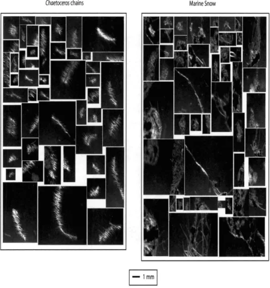
34 1-3 Example VPR images of Chaetoceros chains and marine snow. Fifty ran-

domly selected samples are shown here. .

. . .

.

. . .

. .

. .

.

. . .

.

.

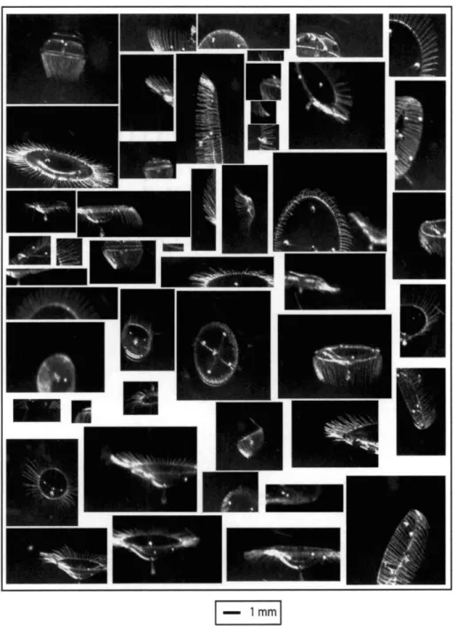
35

1-4 Example VPR images of hydroid medusae. Fifty randomly selected samples are shown here.

. . . .

.

. . . .

.

.

. .

.

. . . . . . .

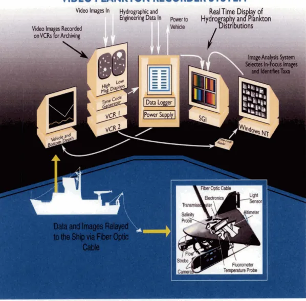
36 2- 1 Video Plankton Recorder system with underwater and shipboard compo-

nents. The VPR is towyoed at ship speeds up to 5 m / s , while video is processed in real-time on board.

.

.

.

. . . .

.

.

. . . .

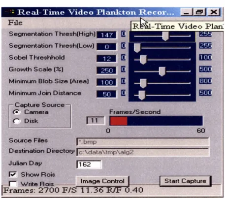
43

2-2 The graphical user interface of real time focus detection program.

. . . . .

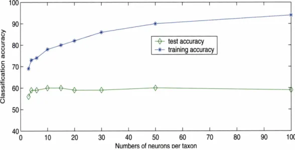
45 3-1 Classification performance with respect to classifier complexity. . .

.

.

59 3-2 Training and test accuracy with respect to classifier complexity.

. . .

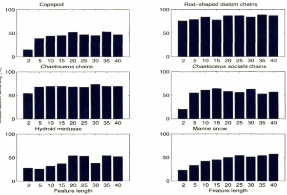
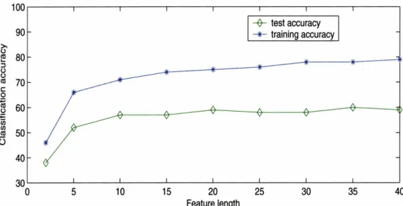
59 3-3 Classification performance as a function of feature length for each taxon. 60

3-4 Training and test accuracy with respect to feature length.

. . . .

.

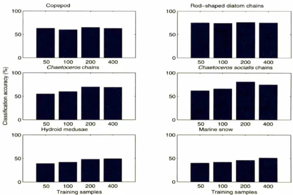
. . 61

3-5 Classification performance as a function of training sample size for each taxon. .

. . . . .

. . .

. . . .

.

. . . .

.

. .

. .

. . . .

.

. . . . .

62

3-7 Comparison between the random initial position of neurons and ran- dom order of presentation order of training samples. IP1

-

different initial position of neurons, random representation order of training sarnples; IP2 - same initial position of neurons, random representation

. . .

order of training samples

3-8 Comparison of different training samples effect on classfication perfor- mance. TSl - different sets of training samples, leave-one-out method; TS2 - different sets of training samples, holdout method; TS3

-

single set training samples, holdout method

. . .

3-9 Mean, upper and lower limit of 95% confidence interval of abundance estimates from LVQ-NN classifiers and that of manually sorted results. Time series abundance plots along the tow path are shown for 6 dom- inant taxa. Data were first binned in 10 second time intervals, and a one-hour smoothing window was applied to the binned data.

. . .

3-10 Illustration of the three most popular decision rules.

x',,

- maximum likelihood decision rule,

xb,,

- maximum a posteriori decision rule,

xb,,

-

minimax decision rule

. . .

3-1 1 Schematic diagram of two pass classification system

. . .

3-12 Comparison of two automatic classification systems with human expert cla,ssified results. Time series abundance plots along the tow path are shown for 6 dominant taxa. Data were first binned in 10 second time intlervals, and a one-hour smoothing window was applied to the binned data

. . .

3- 13 Comparison of automatic classification systems withlwithout statisti- cal correction to human expert classified results. Time series abun- darice plots along the tow path are shown for 6 dominant taxa. Data were first binned in 10 second time intervals, and a one-hour smoothing window was applied to the binned data.

. . .

. . .

4-1 Mean and standard deviation of classification accuracy from different feature presentation methods for each taxon. The abbreviations are as follows: MI - moment invariants, FD

-

Fourier descriptors, SS

-

shape spectrum,

MM

- morphological measurements, CM

-

co-occurrence ma- trices, RL - run length,

EF

-

edge frequency, PS - pattern spectrum, W T

-

wavelet transform. It clearly shows the jump between shape- based features and texture-based features. The pattern spectrum and wavelet transform methods are between shape-based and texture-based methods, their performances lie in between these two group of methods. 102

4-2 Illustrates the problem of non-uniform illunimation on segmentation. (a) the original image, (b) gradient correction of (a), (c) segmentation of (a), (d) segmentation of (b), (e) contour of the largest object from (c), ( f ) contour of the largest object from (d)

. . .

104

4-3 Mean and standard deviation of classification accuracy for moment invariants of different orders for each taxon. M13-7 stands for moment invariants up to order 3-7, which correspond to feature length of 7, 12, 18, 24, and 33 respectively. where MI3 is equivalent tlo Hu's moment invariants. There is no benefit to using high order moment invariants in this dataset.

. . .

105

4-4 Illustrates the problem of using a radius-vector function to encode a,

non-star-shaped plankton image. (a) the original image, (b) the con- tour of the object, (c) the radius-vector function from the contour model of (b), (d) the recovered contour of the object based on radius-

. .

vector function (c) with assumption that the object is star-shaped. 106

4-5

A

comparison between radial Fourier descriptors (RFD) and complex Fourier descriptors (CFD).

. . .

107

4-6 Mean and standard deviation of classification accuracy for co-occurrence matrices of different multi-scale levels for each taxon. The abbrevia- tions CM1-6 stand for co-occurrence matrices of multi-scale levels from 1 to 6, which correspond to feature length of 16, 32, 48, 64, 80, and 96 respectively. The classification accuracy first rises sharply with an increase of multi-scale levels, and reaches top performance with 3-4 multi-scale levels. The performance then drops down slightly as more multi-scale levels are included in the feature set.

. . .

108

4-7

A

comparison between raw co-occurrence matrices (RCM) and statis- tics of co-occurrence matrices (SCM). There is little difference between SCM and RCM.

. . .

109

4-8 Virtual support vector machine test on the co-occurrence matrices method. SCM - statistics of co-occurrence matrices, CCM

-

statis- tics of co-occurrence matrices from original image and its complement, RC;M - statistics of co-occurrence matrices from original image and re- sized images of 0.8 and 1.2. No accuracy gain is obtained by adding virtual samples in the training set.

. . .

110

4-9

,4

comparison of edge frequency features, where EF1 is EF spectrum with linear distance interval from 1 to 40 pixels and two directions formula (horizontal & vertical, and diagonals), EF2 is

EF

with 7 ex- ponential distance interval from 1 to 64 and two directions formula (horizontal & vertical, and diagonals), EF3 is EF with 7 exponential distance interval from 1 to 64 and four directions formula (horizontal, vertical and two diagonals). It is clear that exponential distance inter- val works better than the linear distance interval, and four direction formula works better than two direction formula.

. . .

11 1

4-10 Comparison of run length methods. RL1 - run length statistics pro- posed by Galloway, 5 statistics from each run length matrix, total 20 features for 4 directions. RL2 - extended run length statisitcs by Chu et al., and by Dasarathy and Holder. 11 statistics from each run length matrix, total 44 features for 4 directions. The extended features give a slight better performance for all the taxa.

. . .

112

4-11 Comparison between two implementations of pattern spectrum. PSI -

PS by Vincent, linear and pseudo opening and closing spectra, each has 40 elements, total feature length of 160. PS2 - PS modified from Mei- jster and Wilkinson, horizontal and vertical line opening and closing spectra, and area opening and closing spectra, each has 40 elements, total feature length of 240. PSI outperforms PS2 on all the taxa except marine snow.

. . .

113

4- 12 h4ulti-scale level test for wavelet transform features. WL1-7 stands for features from wavelet transform with multi-scale level from 1 to 7.

.

113

5-1 Comparison of 2 automated classifier with human expert classified re- sults for 6 dominant taxa along the tow timescale. CSF-NN, combined shape-based features and neural network; COM-SVM, co-occurrence features and support vector machine. The data are first binned into 10 second time intervals.

A

1 hour smoothing window is applied to the binned data.

. . .

123

5-2 Comparison of 2 automated classifier with human expert classified re- sults for 6 dominant taxa along the tow timescale. CSF-NN, combined shape-based features and neural network; CSF-SVM, combined shape- based featuresand support vector machine. The data. are first binned into 10 second time intervals.

A

1 hour smoothing window is applied to the binned data.

. . .

124

5-3 Reduction in the relative abundance estimation error rate between COM-SVM and CSF-NN, and between CSF-SVM and CSF-NN. The positjive value indicates that COM-SVM/CSF-SVM is better than CSF- NN, while the negative value indicates COM-SVM/CSF-NN is worse than CSF-NN.

. . . 125

6-1 Schematic diagram of dual-classification system. LVQ: learning vector quantization; NN: neural netowork; SVM: support vector machine

. .

135

6-2 Automatically classified images: comparison of results for

(A,

C) dual- classification system and

(B ,D)

single neural network classifier. The first 25 images classified as (A,B) copepods and (C,D) Chaetoceros socialis by the dual-classification system and LVQ-NN classifier are shown. For taxa having relatively high abundance, such as copepods, both systems yield very similar results (21 out of 25 were the same). In contrast, for taxa having relatively low abundance, such as low- abundance regions of C. socialis, the dual-classification system has

. . .

much higher specificity (fewer false alarms). 139

6-3 Comparison of dual-classification, and manually corrected single NN classification with human expert classified results for 6 dominant taxa along the tow timescale. The data are first binned into 10 second time intervals. A 1 hour smoothing window is applied to the binned data.

.

141

6-4 Comparison of 3 automated classifier with human expert classified re- sults for 6 dominant taxa along the tow timescale. CSF-NN, combined shape- based features and neural network; CSF-SVM

,

combined shape- based features and support vector machine. The data are first binned into 10 second time intervals. A 1 hour s~noothing window is applied to the binned data.

. . . 143

6-5 Reduction in error rate between the dual- and single-classification sys- tems for relative abundance estimation. Positive values indicate that the dual-classification outperforms other methods; negative values in- dicate the opposite. Dual: dual-classificat ion system, CSF-NN: com- bined shape-based features and neural network; CSF-SVM, combined shape-based features and support vector machine.

. . . .

145 6-6 Relationship between specificity and relative abundance for different

false alarm rates. Probability of detection is set to 70%. As false alarni rates become smaller, the range in which the specificity closes to a, constant becomes wider. The dual-classification system has sub- stantially reduced the false alarm rates, so that the specificity of each taxon in the whole study area is close to a constant. This makes fully automatic correctiori possible.

. . . .

. .

. . . .

. .

.

146

List

of Tables

2.1 Comparison of focus detection algorithms from AN9703, high magni- fication camera, video section 1. The numbers are blob counts; prob- ability of detection Pd and probability of false alarm Pf are given as percentages.

. . .

49

2.2 Comparison of focus detection algorithms from AN970:3, high magni- fication camera, video section 2. The numbers are blob counts; prob- ability of detection Pd and probability of false alarm are given as percentages.

. . .

49

2.3 Comparison of focus detection algorithms from AN9703, high magnifi- cation camera, video section 1 after correction. The numbers are blob counts; probability of detection Pd and probability of false alarm Pr a.re given as percentages.

. . .

50

2.4 Comparison of focus detection algorithms from AN9703, high magnifi- cation camera, video section 2 after correction. The numbers are blob counts; probability of detection Pd and probability of false alarm

Pf

are given as percentages.

. . .

51

2.5 Comparison of focus detection algorithms from HALOS, low rnagni- fication camera, video section 1. The numbers are the blob counts; probability of detection Pd and probability of false alarm Pf are given aspercentages.

. . .

52

2.6 Comparison of focus detection algorithms from HALOS, low magni- fication camera, video section 2. The numbers are the blob counts; probability of detection

Pd

and probability of false alarm

Pj

are given . . . as percentages.

3.1 Confusion matrix of an LVQ-NN classifier with distance rejection met- ric using hold-out method. The classifier was trained without marine snow. Column and row heading are coded as: C1, copepod; C2, rod- shaped diatom chains; C3, Chaetoceros chains; C4, Chaetoceros socialis colonies; C5, hydroid medusae; C6, marine snow; C6*, '.unknownv.

.

3.2 Con.fusion matrix of an LVQ-NN classifier with distance rejection met- ric using hold-out method. The classifier was trained without hydroid medusae. Column and row heading are coded as: C1, copepod; C2, rod-shaped diatom chains; C3, Chaetoceros chains; C4, Chaetoceros so- cialis colonies; C5, marine snow; C6, hydroid medusae; C6*, "unknown"

3.3 Confusion matrix of an LVQ-NN classifier with distance rejection met- ric using hold-out method. The classifier was trained without Chaeto- ceros socialos colonies. Column and row heading are coded as: C1, copepod; C2, rod-shaped diatom chains; C3, Chaetoceros chains: C4, hydroid medusae; C5, marine snow; C6, Chaetoceros socialis colonies; C6*, "unknown".

. . .

3.4 Confusion matrix of an LVQ-NN classifier with distance rejection met- ric using hold-out method. The classifier was trained without Chaeto- ceros chains. Column and row heading are coded as: C1, copepod; C2, rod-shaped diatom chains; C3, Chaetoceros socialos colonies; C4, hydroid medusae; C5, marine snow; C6, Chaetoceros chains; C6*, "un- known".

. . .

3.5 Confusion matrix of an LVQ-NN classifier with distance rejection met- ric using hold-out method. The classifier was trained without rod- shaped diatom chains. Column and row heading are coded as: C1, copepod; C2, Chaetoceros chains; C3, Chaetoceros socialis colonies; C4, hydroid medusae; C5, marine snow; C6, rod-shaped diatom chains; C6*: "unknown".

. . .

82

3.6 Confusion matrix of an LVQ-NN classifier with distance rejection met- ric using hold-out method. The classifier was trained without copepod. Column and row heading are coded as: C l , rod-shaped diatom chains; C2, Chaetoceros chains; C3, Chaetoceros socialis colonies; C4, hydroid medusae; C5, marine snow; C6, copepod; C6*, "unknown".

. . .

82

4.1 Mean classification accuracy from different feature representation meth- ods, where the unit is in percent. The abbreviations are as follows: MI - moment invariants, FD

-

Fourier descriptors, SS - shape spectrum,

MM

- morphological measurements, CM

-

co-occurrence matrices, RL - run length, EF

-

edge frequency,

PS

- pattern spectrum, WT - wavelet transform. The best performance for single feature method is the co- occurrence matrices method, which has the average of classification accnra,cy of 74%. It is clear to see that the texture-based methods are superior than shape-based met hods.

. . .

101

4.2 Standard deviation of classification rates from different feature repre- sentation methods, where the unit is in percent. The abbreviations are same asTable4.1.

. . .

101

5.1 Confusion matrix for EN302, VPR Tow 7, based on the co-occurence matrix classifier using hold-out method. Column and row heading are coded as: C1, copepod; C2, rod-shaped diatom chains: C3, Chaeto- ceros chains; C4, Chaetoceros socialis colonies; C5, hydroid medusae; C6, marine snow; C7, 'other'; and Pti, probability of detection. True counts (i.e. human counts) for a given taxa are given in the colunins, while courits by automatic identification (i.e. computer counts) are given in the rows. Correct identifications by the computer are given along the main diagonal, while the off-diagonal entries are the incorrect identification by the computer. Overall accuracy for this classifier was 72%).

. . .

120 5.2 Mean confusion matrix for EN302, VPR Tow 7, based on learning

vector quatization method neural network classifiers built with different randomly selected sets of 200 training ROIs using hold-out method

[34]. Column and row headings are as in Table 5.1. True counts (i.e. human counts) for a given taxa are given in the columns, while counts by attomatic identification (i.e. computer counts) are given in the rows. The correct identifications by the computer are given along the main diagonal, while the off-diagonal entries are the incorrect identification by the computer. Overall accuracy of this classifier was 61%.

. . .

121 5.3 Performance of the classifier with different kernel widths (0)

,

regulation

penalty (C) and kernel types, where d is the polynomial degree and K.

is the kernel coefficient. The recognition rate on the independent test set is shown.

. . .

122 5.4 Kullback-Leibler(KL) distance estimation for difference in abundance

between COM-SVM and hand-sorted and between CSF-NN and hand- sorted. Row headings are as in Table 5.1. The KL distance is dimen- sionless. For two identical abundance curves, the

K L

distance is 0, while for two random distributions, the KL distance is 0.5. Note lower values of COM-SVM than CSF-NN for all four taxa.

. . .

124

6.1 Confusion matrix of the dual-classificat ion system, using the leave-one- out method. Randomly selected images (200 per category) from EN302

VPR.

tow 7 were used to build the confusion matrix. C1: copepods, C2: rod-shaped diatom chains, C3: Chaetoceros chains, C4: Chaetoceros socialis colonies, C5: hydroid medusae, C6: marine snow, C7: other, C7*: unknown, PD: probability of detection

(%),

SP

= specificity

(96).

NA: not applicable. True counts (i.e. human counts) for a given taxa are given in the columns, while counts by classification system are giver1 in the rows. Correct identifications by the computer are given along the main diagonal, while the off-diagonal entries are the incorrect identification by the computer. All data are counts, except in the last rowT and last column, which are percent values. Although images from the "other" category are not needed to train the dual-classification system, they are necessary to evaluate it.

. . .

137 6.2 Confusion matrix of the single LVQ-NN classifier, using the leave-one-

out method. Images used were the same as those in Table 6.1. Ab- breviations as in Table 6.1. All data are counts, except, in the last row and last column, which are percent values.

. . .

140

Chapter

1

Introduction

The vast majority of species in the ocean are plankton. The term plankton was coined by the German scientist Victor Henson at the University of Kiel in 1887 from the Greek word "planktos" , meaning "drifter", to describe the passively drifting or- ganisms in freshwater and marine ecosystems. Many species are planktonic for only part of their lives (meroplankton)

,

including larvae of fish, crabs, starfish, mollusks, corals, etr. Other species are always planktonic (holoplankton), including the many species of phytoplankton and copepods. As primary producers, phytoplankton are responsible for approximately 40% of the annual photosynthetic production on earth. Phytoplankton and their predators, zooplankton, play important roles in processes such as the carbon cycle, the biological pump, global warming, harmful algal blooms and coastal eutrophication. As the base of the ocean food web, plankton play impor- tant roles in sustaining conlmercial marine fisheries. In order to better understand the rriarirle ecosystem, knowledge of the size structure, abundance, mass, and species composition of plankton is crucial. Such measurements are difficult however, since plankton distributions are notoriously patchy and require high-resolution sampling tools for adequate quantification [45, 61, 120, 1081. In spite of over a hundred years of research 11681, our understanding of the structure of aggregations of plankton is still very limited. Taxa-specific abundance at both fine-scale tenlporal and spatial resolution is necessary to assess theoretical ecological models such as those of Riley [134], Fasham [46], Aksnes et al. [2], Lynch et al. [107], Miller et al. [115], and

Carlotti et al. [17].

1.1 Motivation

The advent of new optical imaging sampling systems [31] in the last two decades offers an opportunity to resolve taxa-specifc plankton distribution at much higher spatial and temporal resolution than previously possible with net, pump, and bottle collec- tions. Optical imaging systems rapidly create large amounts of digital image data and ancillary environmental data that need to be analyzed and interpreted. Analyzing the image data can be accomplished using manual processing by trained experts. In addition to the high cost of expert time, such classification processes are tedious and time-consuming, which can cause biased results [28]. On the other hand, advances in pattern recognition and machine learning make it possible to automatically classify plankton images into major taxonomic groups in real time. In this thesis,

I

take this approach and pursue the automatic classification of these images via statistical pattern recognition.

1.2 Statistical pattern recognition

Statistical pattern recognition has been used successfully in a number of applications such as data mining, document classification, biometric recognit ion, bioinformat ics, remote sensing and speech recognition. In statistical pattern recognition, a pattern is represented by a set of measurements, called features. Each pattern then can be viewed as a point in the multi-dimensional feature space. Statistical learning theory is then applied to construct decision boundaries in the feature space to separate the different pattern classes.

A

recognition system is usually operated in two phases: training and classification, as shown in Figure 1-1.

Incoming video from an optical imaging system, in this case a Video Plankton Recorder (VPR) [31, 32, 33, 34, 351, is pre-processed by a focus detection program to extract in-focus objects, called regions of interest (ROI)

,

from each video frame. These

ROIs are saved as Tagged Image File Format (TIFF) image files.

A

subset of these files is manually labeled (identified), and serves as training samples. In the training phase, a set of measurements (features) is computed from each image using different pattern representation methods. Feature extraction is used to linearly combine dif- ferent features and extract the most salient features for classification. Subsequently, to train a classifier, a learning algorithm is employed to partition the feature space into slibspaces belonging to different classes (e.g., species). An import ant feedback path allows a designer to interact with and optimize different pattern representation methods, feature extraction algorithms and learning strategies. The arrows of pattern representation and feature extraction between training and classification phases imply that the same methods are used in classification which are optimized during training. In the classification phase, the trained classifier uses the image-t o-feature mapping, which is learned during training, and assigns an input image to a class based on its locat ion relative to decision boundaries in the feature space.

1.2.1

Features

Features are measurable heuristic properties of patterns of interest. The rationale of pattern representation and feature extraction is to avoid the curse of dimensionality

[a],

the exponential growth of hypervolume as a function of dimensionality. For most practical systems, labeled samples require expert time, thus are expensive to obtain, that is to say, only limited labeled samples are available. In such cases, it has been observed that additional features may degrade the classifier performant:e, which is re- ferred to as the peaking phenomenon [76, 130, 1291. Thus a dimensionality reduction (feature extraction and selection) step is essential, where only a small number of the most salient features are selected to improve the generalization performance (classi- fication performance on samples "unseen" during training) of a classification system. At the same time, this step also reduces the storage requirements and processing time.

Incoming Video

I

- - - I - -

- - -

-I

I

Focus Detect

ion

Manually Sorting

I

Pattern

I

Pattern

Representat

ion

'

Representation

L _I

I

I

Feature

Feature

Extraction

Extraction

I I I

I

~eatureS-vector

I

Feature

Class Label'

Classifier

Classification

4

Learning

I

I I i

I

CLASSIFICATION PHASE

I

TRAINING PHASE

I

I I I

1.2.2

Statistical learning theory

The fundamental work of Vapnik (1 59, 160, 1611 set the foundation for learning from finite samples by using a functional analysis perspective with modern advances of probability and st at ist ics, and revived classical regularization theory. The basic idea of Vapnik's theory is to limit the model capacity by constraining decision boundaries in a "small" hypothesis space, which is dependent on the training samples. This is closely related to classical regularization theory in machine learning and overfit- tinglovertraining in pattern recognition.

More formally, learning from examples can be formulated in the statistical learning theory framework. Suppose we have two sets of variables

x

E

X

c

Rd

and y E Y

c

R.

A

probability density function p(x, y) relates these two sets of variables over the whole domain X

x

Y. We are provided with a data set

Dl

I {(x, y) E

X

x

Y)'.

They are called the training data, and are obtained by sampling the probability density function p(x, y) 1 times. Given the data set Dl, the problem of learning lies in providing an estimator (a classifierla learning machine) as a function fa :

X

-4 Y, which can be used to predict a value of yi given any value of xi E

X.

The functions f,(x) are different mappings with adjustable parameters a.

A

standard way to solve the above learning problem is to define a risk function, which computes the average amount of error (cost) associated with an estimator, then choose the estimator which has the lowest risk. The expected risk of an estimator is defined as,

Here

V

is the loss function, and (Y are adjustable parameters.

A

particular choice of n determines a learning machine. For example, a neural network with fixed architecture is a learning machine, where a are the weights and bias of the network. The target estimator is the function fa* which has minimal expected risk,

fa* (x) = arg min a R( fa)

In practice, the probability density function p(x, y) is unknown, and the expected risk cannot be calculated using Eq. 1.1. To overcome this problem, an induction principle is used to approximate the expected risk from training samples. This is the so-called empirical risk minimization (ERM) induction approach. The empirical risk is defined as,

For limited training samples, the empirical risk is not always a good indicator of the generalization ability of a learning machine. The structural risk minimization principal [160] states that, for any cr E

A

and

1

>

h, the following bound holds with a probability of of at least 1 - q,

The parameter h is a non-negative integer called the Vapnik Chervonenkis (VC) dimension. It is a measurement of capacity of a set of functions. The second term on the right side of Eq. 1.4 is called the

VC

confidence. Consequently, the essential idea of structural risk minimization can be restated thus: for a fixed sufficiently small q, choose the function f,(x) which minimizes the right hand side of Eq. 1.4. For more information on this topic, please refer to Vapnik [160, 1611, Burges [15], and Evgeniou [441.

1.3

An

overview

of

related work

Research on automatic plankton classification has been on-going for many years [82, 81, 135, 69, 25). Early systems worked on images taken under well-controlled lab- oratory conditions, and had not been applied to field-collected images. More recently, artificial neural networks have come to play a central role in classifying plankton im- ages 1145, 12, 27, 150, 149, 154, 281. However, the datasets used to develop and test these classifiers were usually fairly small [150, 281, and, furthermore, only a subset of

distinctive images was chosen to both train and test the classifier. Since a classifier needs to classify all the images from the field, including rare species and difficult ones, even those that cannot be identified by a human expert, the accuracy reported for a. classifier built from only distinctive images will be generally optimistically biased. The classifier performance was usually much worse when it was applied to all field data [34].

The features used in the early systems were mostly shape-based. Jeffries et al. [81] used moment invariants, Fourier descriptors and morphometric relations as features. Although these features worked quite well under well-defined laboratory imaging con- ditions and the overall recognition rate reported by Jeffries et al. was 90% for six taxonomic groups, the system required significant human interaction and was not, suitable for in situ applications.

Initial automatic identification of

VPR

images was carried out using the method described in Tang et al. [150] which introduced granulometry curves (1621, along with traditional features such as moment invariants, Fourier descriptors and morphorne- tric measurements. This method used a learning vector quantization (LVQ) neural network as the classifier [149] and achieved 92% classification accuracy on a subset of VPR images for six taxonomic groups. Only distinctive images were used in training and testing the classifier in this initial study.

A

detailed experiment was conducted in Chapter 3 to show the performance of the system when rare species and diffi- cult images were included in training or testing samples. The average classification performance on the whole dataset was 61% 1341.

The performance disagreement between previous methods [81, 1501 and current study [34] is due to the nature of field-captured images. Unlike the well-controlled laboratory conditions, field images are often occluded (objects truncated at edge of irnage), and shape-based features such as moment invariants and Fourier descriptors are very sensitive to occlusion. In addition, a significant number of field-collected irn- ages cannot be identified by a human expert due to object orientation and position in the image volume1. These unidentifiable images were not used in training and testing 10t).jects can ba hard to identify due to their position in the irrlage volume. If part of the object

the classifier [I501 (although occluded images were included). A recent study by Luo et al. [106] showed that including unidentifiable objects lowered the recognition rate frorn 90% to 75% for their dataset from the shadow image particle profiling evaluation recorder. In order to better estimate species specific abundance, a number of works has shown that it was important to include an "other" [34] or "reject" [58] category. In addition to occlusion, nonlinear illumination of images makes perfect segmenta- tion (biriarization) impossible, even after background brightness gradient correction. Due to the grayscale gradient, the same object can have different segmented shapes depending on where the object is in the field-of-view, thus causing shape-based fea- tures to be less reliable.

Another type of feature we can extract from the grayscale images is a texture-based feature. However, due to the early success of shape-based features on plankton images frorn well-controlled laboratory imaging conditions, texture-based features have not been widely used in plankton image recognition.

Texture-based features were compared against classic shape-based features. The important finding was that the texture-based features were more important than the shape-based features to classify field-collected plankton images. The main cause was that texture-based features were less sensitive to occlusion and projection variance than shape-based features.

1.4

Data

The data set was obtained from a 24-h VPR tow (VPR-7) in the Great South Chan- nel off Cape Cod, Massachusetts, during June 1997 on the R/V Endeavor. The VPR was towed from the ship in an undulating mode, forming a tow-yo pattern between the surface to near bottom. The images were taken by the high magnification cam- era, which had an image volume of 0.5ml. The total sampled volume during the is out of this volurne, the resulting i111age will be occluded. No~lli~lear illuminatio~i rrlakes objects fro111 the dark region more likely to be oc<:luded by global segmentation, a problem corrt?(:table by 1,ackground gradient renloval [35]

deployment was approximately 2.6 m" 2. There were over 20,000 images captured during this tow. All the images were manually identified (labeled) by a human expert into seven major categories (copepod, rod-shaped diatom chains, Chaetoceros chains: Chaetoceros socialis, hydroid medusae, marine snow, and the "other" category, com- prising rare taxa and unidentifiable objects). These are the most abundant categories in this area. In this tow, about 21% of the images belonged to the "other" category. Most of these "other" images were unidentifiable by human experts, and the rest were rare species, including coil-shaped diatom chains, ctenophores, chaetognaths, poly- chaetes and copepod nauplii (see Davis et al. [34]). The manual identification took several weeks to accomplish. Representative samples (images) are shown in Figs. 1-2, 1-3, arid 1-4. Manual labels were treated as ground truth for comparing different classification results.

1.5

Thesis overview

This thesis consists of seven chapters and is organized as follows.

C h a p t e r 1: Introduction- I introduce the importance of automatic classifica-

tion of plankton images. I then set up the problem in the framework of statistical pattern recognition, and review basic concepts on statistical learning and related work. Finally, I describe the data set used in this thesis.

C h a p t e r 2:

Data

acquisition-

I

give an overview of water column plankton samplers, and then focus on the Video Plankton Recorder

(VPR).

I develop three algorithms of focus detection and examine four short sections of video.

I

then compare the results from three algorithms to the manual examination in terms of probability of detection and probability of false alarm.

C h a p t e r 3: Classification method: analysis a n d assessment-

I

present a detailed assessment of the application of a learning vector quantization neural network (LVQ-NN) on the data set. More specifically,

I

examine the following: classifier 2As pointed out in Davis et d. [35], although the volurrle irnitged t1-y VPR is srrlall conipared to thct volume filtered by a planktori net,, the VPR still can provide an equivale~it or bet,t,er estirrlate of

Copepods Chaetoceros socialis colonies

Rod-shaped Diatom Chains Other

Figure 1-2: Example VPR images of copepods, rod-shaped diatom chain, Chaetoceros socialis colonies and the "other" category. Fifty randomly selected samples are shown here.

Choetoceros chains Marine Snow

Figure 1-3: Example VPR images of Chaetoceros chains and marine snow. Fifty randomly selected samples are shown here.

Hydroid Medusae

Figure 1-4: Example VPR images of hydroid medusae. Fifty randomly selected samples are shown here.

co~nplexity, feature length, learning curve, presentation order of training samples, and different training samples. Next I propose a two-pass classification system and compare the result with both the single LVQ-NN classifier and the single LVQ-NN classifier with statistical correction. Finally, I modify the LVQ-NN to have an outlier rejection metric based on the mean distance of correctly classified training samples.

C h a p t e r 4: P a t t e r n presentation- First I give an overview of pattern repre- sent ationlfeature measurement met hods. I group the pattern presentation met hods into three major groups, namely, shape-based, texture-based, and other met hods.

I

then conduct a comparison study between shape-based features and texture-based feat.ures on a random set of the plankton data.

I

find the texture-based features are more important than shape-based features to classify field-collected images.

I

keep the comparison results as guidelines for choosing different feature presentation methods in the later chapters.

C h a p t e r 5: Co-occurrence matrices a n d s u p p o r t vector machine- I inves- tigate the multi-scale co-occurrence matrices, and support vector machines to classify the plankton image data set. From Chapter 4, I find that texture-based features are more robust for classifying field-collected plankton images with occlusions, nonlin- ear illurninat ion and project ion variance.

I

demonstrate that by using features from multi-scale co-occurrence matrices and soft margin Gaussian kernel support vector machine classifiers, a 72% overall probability of detection can be achieved compared to that of 61% from a neural network classifier built on combinded shape-based fea- tures. Subsequent plankton abundance estimates are improved in regions of low relative abundance by more than 50%.

C h a p t e r 6: D u a l classification system-

I

incorporate a learning vector quan- tization neural network classifier built from combined shape-based features and a support vector machine classifier with texture-based features into a dual-classification system. The system greatly reduces the false alarm rate of the classification, thus extends the regions where the specificity curve of classification is relative flat, which makes global correction of abundance estimation possible. After automatic correction, the abundance estimation agrees very well both in high and low relative abundance

regions. For the first time,

I

demonstrate an automatic method which achieves abun- dance estimation as accurately as human experts.

Chapter 7: Conclusions and future work- First, I summarize the major corltributions of this thesis, and then discuss the possibility of extending the existing system t o color or 3-D holographic images.

Chapter

2

Data Acquisition

111 this chapter,

I

first overview water column plankton samplers in Section 2.1, then decribe one specific optical sampler, the Video Plankton Recorder, in detail in Section 2.2. The main focus of this chapter is to discuss the focus detection program, which is discussed in Section 2.3. I develop three new focus detection algorithms, and compare them against human judgment on four video sections from

VPR.

This is the first quantitative study of focus detect ion.

2.1

Water column plankton samplers

The development of quantitative zooplankton sampling systems can be traced back to the late 19th and early 20th centuries. Non-opening/closing nets [67, 831, simple openiilg/closing nets [71] and high-speed samplers [4] all began to be employed at, that tirne. All these systems have evolved with advances in technology, and are still widely used for plankton survey programs. For example, non-opening/closing nets, such as the Working Party 2 (WP2) net [49], modified Juday net [I], and Marine Resources Monitoring Assessment Prediction (MARMAP) Bongo net [126] are still used in large ocean surveys; simple opening/closing nets similar to those developed by Hoyle [71], Leavitt [96], Clarke and Bumpus [24] are still nianufactured and used; high-speed samplers are also in use, such as the continuous plankton recorder [60], which has evolved over 30 years, and become the main sampling system in the North

Atlantic plankton survey 11641.

Since the 1950s, the concept of plankton patchiness has been well established, and it triggered the development of closing cod-end systems and multiple net systems in the 1950s and 1960s. Cod-end samplers such as the Longhurst-Hardy plankton recorder [103] had problems with hang-ups and stalling of animals in the net which caused smearing of the distributions of animals and loss of animals from the recorder box 1631. The system was modified by Haury et al. to reduce these sources of bias and used to study plankton patchiness in a variety of locations 162, 641. Multiple net' systems [169, 1721 were developed to fix these problems by opening and closing nets in specific portions of the water column.

With the advances in charge-coupled device ( CCD) and computer technology, the 1980s and 1990s saw a boom of optical plankton sampling systems. Optical systems have a number of advantages over net-based systems. The optical systems can provide much finer vertical and horizontal spatial resolution than the net-based sy~t~erns. Optical systems have the potential to provide abundance estimates at short temporal intervals along the tow path 1321. Furthermore, delicate and particulate matter that may be damaged by net collection can be quantified by optical systems [5, 381. Image-forming systems have the potential to map taxa-specific distribution in real time (341. However, optical systems usually have a smaller sampling volume than net-based systems given the same tow length. Thus rare organisms may remain undetected with optical sampling systems.

Optical systems can be divided into two categories depending on whether the sys- tem produces images of organisms or not. Non-image-forming systems such as the optical plankton counter [68] use the interruption of a light source to detect and esti- mate particle size. The family of image-forming systems has grown continuously since 1990. The Ichthyoplankton Recorder (IR) [50, 991, Video Plankton Recorder (VPR) [31], Underwater Video Profiler (UVP) [55], Optical-Acoustic Submersible Imaging System (OASIS) 1751, In situ Video Camera [152], FlowCam 11441, Holocamera [88], Shadowed Image Particle Profiling and Evaluation Recorder (SIPPER) (1381, Zoo- plankton Visualization and Imaging System (ZOOVIS) [lo], HOLOCAM [166], In

situ Crittercam [147], and Optical Serial Section Tomography (OSST) [48] all belong to this category. In this thesis, images from the VPR. were used. However, the algo- rithms developed in this thesis are generic, and readily applied to images from other optical plankton sampling systems.

Another group of plankton sampling systems is acoustic-based [170, 471. Such systems use acoustic backscattering to measure the size distribution of particles and plankton. Hybrid systems also have been developed, combining optical and acous- tic sampling, e.g., the VPR has been combined with multifrequency acoustics on the BIo-Opt ical Mult i-frequency Acoustical and Physical Environment a1 Recorder (BIOI\.IAPER,-11) [173]. For more detailed review of plankton sampling systems, please refer to Wiebe and Benfield [168].

Imaging plankton at sea while towing the sampler through the water at a 1-6 m/s, requires a combination of magnifying optics, short exposure time, and long working distance ( 0.5 m). The long working distance is needed to minimize detection and avoidance of the sampler by the plankton. The short exposure time (e.g., 1 ps) is obtained using a strobe. The density of pixels on the CCD array, together with the need to image enough details of the individual plankton to identify them, limits the camera's field-of-view (FOV) to 1 cm for most mesozooplankton. For a depth of focus of 3 n n , the image volume is 3 cm" and video rate of 60 fields per second (FPS), yields 0.18 liter of water imaged per second. Given a typical coastal concentration of rnesozooplankton of 10 individuals per liter, the time between individual sightings is 0.55 seconds, and at 60 FPS, there are 33 video fields between sightings. Thus, only a small fraction of the video fields will contain mesozooplankton. For typical survey periods of several hours or days, the volume of video data collected is much too large for human operators to process manually. (For example, VPR has the bandwidth of 6 Mb/s or 518 Gb/day). Automatic pre-processing of the data is essential [31, 331. I11 this chapter, I focus on one such pre-processing method called focus detection. Before discussing this met hod, a detailed description of the VPR is necessary.

2.2

Video Plankton Recorder

The VPR system includes an underwater unit with video and environmental sensors, and a deck unit for data logging, analysis and display (Figure 2- 1). The underwater unit, has a video system with magnifying optics that images plankton and seston in the size range of 100 microns to several centimeters [31, 33, 34, 351. The initial design [31] had four SONY XC-77 CCD cameras configured to simultaneously image ~oricent~ric volumes at different magnifications. The fields of view of the four cameras were 0.7 x 0.56,3 x 2.4,5 x 4, and 8

x

6.4 cm2 respectively. Depths of field were adjustable by different aperture settings. The sampled image volumes in each field ranged from 0.5 ml to 1 liter depending on the optical settings. The modified system [33, 341 had two analog video cameras of high and low magnification respectively. The high magnification camera had an image volume of about 0.5 ml per field, while the low magnification camera had an image volume of about 33 ml per field. Early testing determined that these two cameras provided the most useful information. The high-magnificat ion camera provided detailed images permitting identification to the species level, while the low-magnification camera imaged larger organisms such as ctenophores and euphausiids. Positioning the image volume at the leading edge of the tow-body and having a wide separation of the cameras and strobe, permitted imaging of animals in their natural undisturbed state.

The images studied in this thesis came from the high magnification camera, which had a pixel resolution of about 10 microns. The cameras were synchronized at 60 fields per second to a xenon strobe1. The VPR also included a suite of auxiliary sensors that measured pressure, temperature, salinity, fluorescence, beam attenuation, down- welling light, pitch, roll, velocity and altitude. The environmental and flight control sensors were sampled at 3 to 6 Hz. The underwater unit was towyoed at 4 ms-I using a 1.73 cm diameter triple-armor electro-optical cable. Video and environmental data from the towbody were received via a fiber optic cable into the data logging and

l ~ h i : c:urrent systenl has a single 1008 x 1018 digital camera with field of view fro111 5 x 5 m 7 r s 2 to 20 x 20 rrsrrr2, and the depth-of-field is objectively calibrated using a tethered orgarlis111. The images wt?rc: sampled at 30 frarries per seco~id [35]

Figure 2- 1 : Video Plankton Recorder system with underwater and shipboard components.

The VPR is towyoed at ship speeds up to 5 m/s, while video is processed in real-time on board.

focus detection computer on the ship.

The deck unit consisted of a video recording/display system, an environmen- tallnavigational data logging system, an image processing system and a data dis- play system. Video was time-stamped at 60 fields per second and recorded on SVHS recorders. The video time code was synchronized with the time from the P-code Global Positioning System. Latitude and longitude were logged with video time code and environmental data a t 3 Hz on a personal computer and a Silicon Graphics Inc

(SGI) workstation.

2.3

Focus Detection

Video with time code from the high magnification camera was sent to the focus detect ion system, which included an image processor interfaced to a computer. Video was first digitized at field rates, then in-focus objects were detected using an edge detection algorithm. The regions of interest (ROI) were saved to the hard disk as tagged image format files using the video time code as the filename.

2.3.1

Objective

The main objective of the focus detection algorithm is data reduction. The video comes in from the video camera at 60 fields per second. As discussed above, a large proportion of fields are devoid of in-focus objects. Early systems required a human operat,or to scan through all the video fields to determine when an in-focus organism was observed and to what species it belonged. Such processes were very slow and tedious, and introduced a source of subjective error when a line was drawn between in-focus and out-of-focus objects. This line could vary from person to person, and from time to time. The objective of the focus detection algorithm is to replace the l.iurnan operator with a program which objectively extracts in-focus objects from the video irnages. The focus detection algorithm is required to extract as many in-focus objects as possible, while picking up as few out-of-focus objects as possible, all in real time. More formally, the focus detection program needs to have a high probability

of detection, while maintaining a low probability of false alarm.

A

graphic user interface (GUI) is available to select parameters such as segmentation threshold, Sobel threshold, growth scale, minimum blob size, and minimum join distance (Figure 2-2). Choosing different parameters sets the tradeoff between the probability of detection and the probability of false alarm.

A

high probability of detection usually related with a high probability of false alarm, which increased the level of difficulty of the subsequent classification problem and required more disk space. On the other hand, low probability of false alarm was related with a low probability of detection. The effective sampling volume was reduced.

A

compromise between the probabilities of detection and false alarm needed to be made by adjusting the controlling parameters in the focus detection GUI.

I

'; Real-Time Video PlanktonRecor..

2.3.2

Method

In-focus object detection involves brightness correction, segmentation, labeling, size thresholding, edge detection, edge thresholding, coalescing and ROI generation. In- coming videos are dynamically adjusted to correct temporal changes in mean bright- ness by shifting the mean brightness of each video frame to a certain value. Transla- tion instead of scaling is used in this normalization step to avoid changing brightness gradients within the frame. Brightness correction is followed by segmentation which involves binarization of gray-scale irnages into binary images. Pixels with brightness above the threshold value are set as foreground while the rest of the pixels are set as background. After segmentation, a connectivity algorithm is used to check how the foreground pixels connect to form blobs. The distinct blobs then are labeled from 1 to N , where N is the number of blobs present in the video field. Due to the imaging environment, there are many small blobs present in each frame. Since small objects are impossible to identify in the later processing and require much processing time, a size threshold is imposed, and consequently blobs below a minimum number of pixels are ignored. A rectangular bounding box is placed around each blob which passes size thresholding. A Sobel operator is applied to each blob to calculate the brightness gradient of the subimages. The small gradients in the subimages are considered to be noise instead of real edges, and the gradients of each subimage are further thresholded in order to suppress this noise.

Three in-focus algorithms are developed based on these thresholded gradients. If the blob is in-focus, the center position and size are saved. After in-focus checking

011 all the blobs from one field is completed, the bounding box of an in-focus blob is

extendedfshrunk according to the GUI growth scale setting. Planktonic organisms usually are partially transparent or translucent. When binarized, one organism often breaks into several blobs. A coalesce operation is applied to group the close in-focus blobs into one blob. Two or more blobs are considered to coalesce if there are overlaps after the bounding boxes relax or if the central distance between them is below a user- defined value on GUI. The resulting subimage inside the bounding box is called region