Subcritical dynamo bifurcation in the Taylor Green flow

HAL Id: hal-00163353

https://hal.archives-ouvertes.fr/hal-00163353v2

Preprint submitted on 23 Jul 2007

HAL is a multi-disciplinary open access

archive for the deposit and dissemination of

sci-entific research documents, whether they are

pub-lished or not. The documents may come from

teaching and research institutions in France or

abroad, or from public or private research centers.

L’archive ouverte pluridisciplinaire HAL, est

destinée au dépôt et à la diffusion de documents

scientifiques de niveau recherche, publiés ou non,

émanant des établissements d’enseignement et de

recherche français ou étrangers, des laboratoires

publics ou privés.

Subcritical dynamo bifurcation in the Taylor Green flow

Yannick Ponty, Jean-Phillipe Laval, Bérengère Dubrulle, François Daviaud,

Jean-François Pinton

To cite this version:

Yannick Ponty, Jean-Phillipe Laval, Bérengère Dubrulle, François Daviaud, Jean-François Pinton.

Subcritical dynamo bifurcation in the Taylor Green flow. 2007. �hal-00163353v2�

hal-00163353, version 2 - 23 Jul 2007

Laboratoire Cassiop´ee, CNRS UMR6202, Observatoire de la Cˆote d’Azur, BP 4229, Nice Cedex 04, France

2

Laboratoire de M´ecanique de Lille, CNRS UMR8107, Bd P. Langevin, 59655 Villeneuve d’Asq, France

3

Service de Physique de l’Etat Condens´e, CNRS URA 2464, CEA Saclay, 91191 Gif-sur-Yvette, France

4

Laboratoire de Physique, de l’ ´Ecole Normale Sup´erieure de Lyon, CNRS UMR5672, 46 All´ee d’Italie, 69007 Lyon, France

We report direct numerical simulations of dynamo generation for flow generated using a Taylor-Green forcing. We find that the bifurcation is subcritical, and show its bifurcation diagram. We connect the associated hysteretic behavior with hydrodynamics changes induced by the action of the Lorentz force. We show the geometry of the dynamo magnetic field and discuss how the dynamo transition can be induced when an external field is applied to the flow.

PACS numbers: 47.65.-d,91.25.Cw

Larmor [1] is generally credited for suggesting that the magnetic field of the Sun (and, by extension, that of planets and other celestial bodies) could be due to dy-namo action – i.e. self-generation from the motions of an electrically conducting fluid. This principle has received much theoretical support [2] since then and has recently been validated by experimental observations [3, 4, 5, 6]. Dynamo action results from an instability: when the flow magnetic Reynolds number RM exceeds a critical value

Rc

M, the null magnetic field state looses its stability to a

non-zero magnetic field state. Because of the low value the magnetic Prandtl number of the considered fluids, this instability usually happens on a turbulent (noisy) basic state and the choice of an order parameter can be ambiguous [7]. However, we can assume that the usual concepts of stability theory apply (cf. later) and study if the transition is supercritical or subcritical [8]. In most models and in all experiments, this bifurcation is super-critical: Rc

M is a unique number, albeit flow dependant.

For instance Rc

M ∼ 14 and R

c

M ∼ 18 for the constrained

Karlsruhe and Riga experiments, while Rc

M ∼ 32 for the

fully turbulent VKS dynamo [5]. On the other hand, the dynamo bifurcation may also be subcritical partic-ularly because the action of a growing magnetic field is supposed to reduce hydrodynamic turbulence and main-tain dynamo action for lower RM values. In fact, the

transition can be globally subcritical if the basic state experiences instability with respect to finite amplitude perturbations [9]. A characteristic hysteretic behavior is then associated to the bifurcation, and the dynamo op-erates for a range of lower values RgM < RM < RcM.

Subcriticality has been discussed in MHD Alpha-Omega dynamical systems [10, 11] and also for numerical simula-tions of convective dynamos in spherical geometries [12]

In this Letter, we study the dynamo bifurcation using full MHD simulations, generated in a 3D-periodical do-main, by the Taylor Green forcing [13]. At low Reynolds numbers, this flow has several metastable hydrodynamics states [14]. At higher Reynolds numbers, it has a well

de-fined mean flow structure with superimposed intense tur-bulent fluctuations. Recent studies of the linear problem have shown that, while the dynamo thresholds may run-away in flows generated by random forcing [15], a dynamo is observed at all kinetic Reynolds numbers [16, 17, 18] in the Taylor-Green flow. We study the fully nonlinear regime and report here evidence of the subcriticality of the bifurcation.

Using standard direct numerical simulation (DNS) pro-cedures we integrate pseudospectrally the MHD equa-tions in a 2π-periodic box:

∂v ∂t + v · ∇v = −∇P + j × B + ν∇ 2 v+ F, (1) ∂B ∂t + v · ∇B = B · ∇v + η∇ 2 B, (2)

together with ∇ · v = ∇ · B = 0; a constant mass density ρ = 1 is assumed. Here, v stands for the velocity field, B the magnetic field (in units of Alfv´en velocity), j = (∇×B)/µ0the current density, ν the kinematic viscosity,

η the magnetic diffusivity and P is the pressure. The forcing term F is given by the TG vortex

FTG(k0) = 2f (t)





sin(k0 x) cos(k0 y) cos(k0 z)

− cos(k0x) sin(k0 y) cos(k0z)

0



 ,

(3) implemented here at k0 = 1. In the sequel, we consider

two types of forcing: one in which f (t) is set to a constant – this is the constant force forcing (f (t) = 1.5) consid-ered in [16]. In a second one 2f (t) is set by the condi-tion that the (1, 1, 1) Fourier components of the velocity remains equal to the Taylor-Green vortex – this is the constant velocity forcing considered in [17]. For the lin-ear instability problem, both forcing yield the same value of Rc

M [16, 17]. We now explore the non-linear regime,

as well as the response to finite amplitude perturbations. Three control parameters drive the instability: the mag-netic and kimag-netic Reynolds numbers and the amplitude

2 of an external magnetic field B0 when applied.

RM = v0 rmsπ η RV = v0 rmsπ ν Λ = B0 v0 rms . (4)

In the definition of the Reynolds numbers, the charac-teristic length scale is set to π, the size of a TG cell when k0 = 1. The characteristic speed v0rms is

com-puted from hydrodynamic runs in which the Navier-Stokes equation is not coupled to the induction equa-tion, v0

rms = hp2EV(t)it. Here EV is net kinetic energy

EV(t) and h·itstands for averaging in time (1/T

RT

· dt). Likewise, in dynamo runs, the intensity of the magnetic field is estimated from the net magnetic energy EM(t),

as b = hp2EM(t)it.

Previous works [17, 18] have explored the response of TG flows to infinitesimal magnetic perturbations, as a

function of the kinetic Reynolds number RV. It was

found that at any RV, there exists a critical RcM above

which perturbations grow exponentially. This is illus-trated in Fig. 1 for a run at RV = 563 and RM = 281

above the critical value Rc

M = 206. The initial magnetic

field perturbation – with an energy level EM = 10−17 –

first grows exponentially. At time t ∼ 300, the magnetic field has reached sufficient amplitude so that it can react back onto the velocity field, saturate the instability and reach a statistically stationary state, with approximate equipartition EM ∼ EV. Note that times are given here

in units of equation (1), for which 1 is very close to one eddy turnover time of the flow (TNL = π/vrms0 ∼ 1.17).

This transition from infinitesimal perturbations builds the (solid) red curve in Fig.2.

We have then quenched the system: at t = 1000, the magnetic diffusivity η is suddenly increased by a factor of 4, lowering RM below RcM. After a short transient, both

EV and EM decrease and reach a second statistically

sta-tionary state, with a non zero magnetic energy – a new dynamo state, for which equipartition is reached again (Fig. 1). This behavior is an evidence for global sub-criticality [9]. The different levels of fluctuations in the two regimes suggest the possibility of different dynamo states, depending on the magnetic field or on history of the system.

As subcritical bifurcations are also associated with hys-teresis cycles, we have repeated the quenching procedure starting from the same dynamo state A (obtained at t = 1000 at RV = 563 in Fig. 1) for increasing values of η,

i.e. for decreasing RM values. The (time-averaged)

mag-netic and kimag-netic energy obtained after rearrangements are then recorded, and results summarized in Fig. 2 by the curve in the B0= 0 plane. Starting from point A, one

can sustain the dynamo after quenching through points A2 to A9, until a value RgM substantially lower than R

c M

(at A9, RM = 70 compared to RM = 211 in A3).

We have investigated further the system behaviour along the cycle by monitoring the spatial structure of

0 500 1000 1500 0 2 4 6 8 10 time Kinetic energy η=0.03 η=0.12 0 500 1000 1500 0 2 4 6 8 10 time Magnetic energy η=0.03 η=0.12

FIG. 1: After a dynamo is self-generated from infinitesimal perturbations, the induction equation is quenched at t = 1000 by a four-fold increase of the magnetic diffusivity. It corre-sponds to a sudden change from A to A9 – cf. Table I.

Point η RM b LB vrms LU A 0.03 281 2.8 5.2 2.7 3.0 A2 0.035 241 2.8 5.3 2.5 3.0 A3 0.04 211 2.8 5.4 2.5 2.9 A4 0.05 169 2.7 5.5 2.3 2.9 A5 0.07 121 2.6 5.7 2.0 2.9 A6 0.08 106 2.5 5.7 1.8 2.9 A7 0.09 94 2.4 5.7 1.7 2.9 A8 0.1 84 2.0 5.5 1.7 2.9 A9 0.12 70 1.6 5.1 1.9 3.0 A10 0.15 56 0.0 0.0 2.7 2.6

TABLE I: For each regime: root mean square amplitude of the magnetic/resp.velocity fields b = hp2Em(t)i , vrms=

hp2Ev(t)i, integral scale of the magnetic/resp.velocity fields LB= hP EB(k, t))/ki , LU= hP EV(k, t))/ki – E(k, t) is

the uni-dimensional energy spectra.

the magnetic and kinetic energies, so as to detect possi-ble changes in the flow structure. In a first regime, until point A7, the kinetic energy (and hence vrms, i.e. the

turbulence intensity – see Table I) decreases and so does the magnetic energy – equipartition being essentially pre-served. Past A8, changes occur: EV starts to increase

abruptly, while EM continues to decrease, resulting in a

decreasing ratio EM/EV – see also Fig.4. Other global

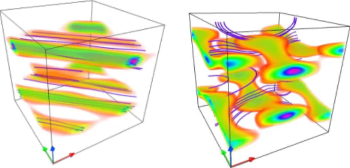
quantities are also changing along this branch (see Table I). It corresponds to a modification in the spatial struc-ture of the magnetic energy. As can bee seen in Fig. 3, the dynamo modes in A7 and A8 are different. At A7,

the dynamo has a structure with magnetic energy ‘tubes’ in which the field line are concentrated along diagonal di-rection (aligned with the energy structures). In A8, the dynamo has a magnetic energy with a wavy shape and the field line are no longer parallel to the energy struc-tures. In fact, the geometry of the A8 and A9 dynamo modes is reminiscent of the low kinematic mode of the TG dynamo[18]. 0 50 100 150 200 250 300 350 400 0 0.05 0.1 0 0.5 1 1.5 2 2.5 3 b A0 A A3 A10 A9 A8 A7 C C’ A’ B 0 R M D

FIG. 2: Bifurcation curves and hysteresis cycles when an ex-ternal magnetic field is applied (full diamond symbols) or without one (full circle symbols). In this case, the subcritical quenched states (see text) form the red line. Jumps between the two branches link A to A′_{and C to C}′_.

FIG. 3: Volume rendering (75% of max(b)) of the magnetic energy and magnetic field lines [19], for the normalized mag-netic field hB(x, t)/B(t)i averaged in time during the run; (left) point A7 and (right) point A8.

As turbulence influences the dynamo, we have re-peated the above sequence of quenching at varying

ki-netic Reynolds numbers RV. The result is shown in

Fig. 4. We first observe that the hysteretic behavior per-sists as RV is lowered. In addition, the hysteresis cycle

width, Rc M− R

g

M, decreases with RV. It is interesting to

compare their locations with respect to the dynamos win-dows evidenced in [17, 18] for the Taylor-Green forcing. As shown in Fig. 4, Rg_M values are almost independent of RV and lie close to the beginning of the first kinematic

dynamo mode. Of course, the onset Rc

M switches from

the kinematic low branch to the kinematic high branch as RV increases (and turbulence develops) [17, 18]. The

width of the dynamo cycle is thus linked to the evolution of the Rc

M(RV) curve.

The above results were obtained with a constant force scheme. We have also repeated the quenching procedure using the constant velocity forcing. As can be seen in Fig. 4 (black curve / diamonds symbols), the hysteretic behaviour remains, but the transition towards the non-dynamo state is more abrupt. Another difference con-cerns the response to quenching; with a constant velocity forcing we observed a lower magnetic saturation level b. Those differences could be explained by a change in hy-drodynamics properties such as the fluctuation level, at the same Reynolds number. In addition, when the veloc-ity is kept constant there may be less possibilveloc-ity for the Lorentz force to change the flow.

0 50 100 150 200 250 300 350 101 102 103 104 0 0.5 1 1.5 2 2.5 R M R V b

FIG. 4: Hysteresis cycle for different Reynolds numbers and forcings – constant force (red, blue) and constant velocity (black). The thick solid line in the b = 0 plane is the linear instability Rc

M vs RV from dynamical runs; the kinematic

dynamo windows [18], RM ∈ [50, 110] and RM > 320, are

delimited by the thick dotted lines.

Finally, we have checked the influence of finite ampli-tude external perturbations on the hysteresis cycle by ap-plying an external magnetic field of amplitude B0= 0.07

in the vertical direction. The result at RV = 563 is shown

by the blue line in Fig. 2. When comparing to the B0= 0

case (red curve), two effects are readily observed : (i) the hysteresis cycle is shortened and this is essentially due to a decrease in the onset Rc

M from infinitesimal

perturba-tions; (ii) the amplitude of the magnetic energy in the dy-namo is decreased, as lower b values are obtained. These observations are indications that the external magnetic field has mediated a transition towards another equilib-rium state [14]. The transition towards this second equi-librium state is quite robust: one can also obtain it by switching on the vertical magnetic field starting from a state with a well-developed dynamo (jump from A to A′

4 an applied magnetic field and switching it off, one returns

to the zero-magnetic field hysteresis curve (jump from C to C′ _{in Fig. 2).}

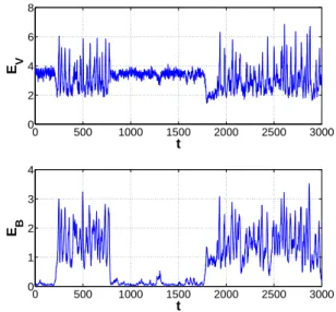
A less deterministic behaviour is observed when the system is operated in the vicinity of point D – shown along the blue curve in Fig.2. At this point, the sys-tem is operated at a magnetic Reynolds number slightly smaller than the linear threshold (93.8 compared to about 100) and one observes that the the systems sponta-neously switches between dynamo and non-dynamo pe-riods, as shown in Fig.5. This is reminiscent of the “on-off” bifurcation scenario sometimes proposed for the dy-namo [20, 21, 22, 23] at high RV. It has been observed in

models [24] and experimental [25] versions of the Bullard dynamo [26], and possibly in turbulent fluid dynamos [6]. We note in Fig.5 that the kinetic energy has stronger fluc-tuations during the dynamo periods.

0 500 1000 1500 2000 2500 3000 0 2 4 6 8 t E V 0 500 1000 1500 2000 2500 3000 0 1 2 3 4 t E B

FIG. 5: Evolution on time of the kinetic (EV) and magnetic

energy (EB) when the flow is operated in the immediate

vicin-ity of point D – see Fig.2.

To summarize, we have evidenced in the TG flow sev-eral features characteristic of subcriticality of the dynamo instability. At variance with usual dynamical system, this behaviour is obtained in a fully turbulent system, where fluctuations are of the same order of magnitude as the mean flow. We may remark that in this case, the tra-ditional concept of amplitude equation may be ill-defined and one may have to generalize the notion of ‘subcritical transition’ for turbulent flows. Another feature is the sen-sitivity to perturbations of the order parameter through the application of an external magnetic field. The pertur-bation mainly acts through macroscopic changes in the system configuration (perturbation of the velocity field), allowing lower thresholds for dynamo instability. These findings open new perspective for experimental dynamos.

For the TG flow, we observe a decrease of the dynamo threshold by as much as 57 percent, with an external

applied field of B0 = 0.07. We have also found that

changes in the geometry of the dynamo states in the subcritical branch are consistent with the coexistence of several metastable hydrodynamics states [14]. Prelimi-nary observations in the VKS experiment also point to the existence of subcritical dynamos in the presence of global rotation [27], a feature also noted in some numer-ical models of the geodynamo [12].

AcknowledgementsWe acknowledge useful discussions

with A. Pouquet and P. Mininni, R. Jover and team mem-bers of the VKS collaboration. Computer time was pro-vided by IDRIS and the Mesocentre SIGAMM at Obser-vatoire de la Cˆote d’Azur. This work is supported by the French GDR Dynamo. YP thanks A. Minuissi for computing design assistance.

[1] J. Larmor, Rep. Brit. Assoc. Adv. Sci, 159-160, (1919). [2] H. K. Moffatt, “Magnetic field generation in electrically

conducting fluids”, (Cambridge U. Press, 1978); [3] A. Gailitis et al., Phys. Rev. Lett. 86, 3024 (2001) [4] R. Stieglitz and U. M¨uller, Phys. Fluids 13 561 (2001) [5] R. Monchaux et AD., Phys. Rev. Lett. 98 044502, (2007) [6] M. Berhanu et al., Europhys. Lett. 77, 59001 (2007) [7] R. Berthet et al., Physica 174D, 84 (2003)

[8] P. Manneville, “Dissipative Structures and Weak Turbu-lence”, (Academic Press, Boston, 1990)

[9] O. Dauchot, P. Manneville, J. Phys. II 7(2), 371 (1997) [10] K. A. Robbins, Proc. Nati. Acad. Sci. USA 73(12),

4297-4301 (1976)

[11] S. Fedotov, I. Bashkirtseva and L. Ryashko, Phys. Rev. E 73, 066307 2006.

[12] V. Morin, Ph. D. Thesis, University Paris VI (1999) ; U.R. Christensen, P. Olson and G.A. Glatzmaier, Geo-phys. J. Int., 138, 393 (1999).

[13] M. Brachet, Fluid Dyn. Res. 8, 1 (1991); C. Nore et al., Phys. Plasmas 4, 1 (1997)

[14] B. Dubrulle et al, to appear in NJP (2007).

[15] A.A. Schekochihin et al., New J. Physics 4, 84 (2002); A.A. Schekochihin et al., Phys. Rev. Lett. 92, 054502 (2004); A. B. Iskakov et al., arXiv/astro-ph/0702291 [16] Y. Ponty et al., Phys. Rev. Lett. 94, 164512 (2005) [17] J.-P. Laval et al., Phys. Rev. Let. 96 204503 (2006) [18] Y. Ponty et al., New J. Phys. (2007)

[19] Imagery using VAPOR code (www.vapor.ucar.edu) [20] S. Lozhkin, D. Sokoloff, P. Frick, Astronomy Reports

43_{(11), 753 (1999)}

[21] D. Sweet et al. Phys. Rev. E 63, 066211 (2001)

[22] N. Leprovost and B. Dubrulle, Eur. Phys. J. B, 44 395 (2005).

[23] M. D. Nornberg et al. Phys. Rev. Lett. 97, 044503 (2006) [24] N. Leprovost, B. Dubrulle, F. Plunian,

Magnetohydrody-namics 42, 131 (2006)

[25] M. Bourgoin et al., New J. Phys. 8, 329, (2006) [26] E. C. Bullard, Proc. Camb. Phil. Soc 51, 744 (1955) [27] VKS team, private communication.