HAL Id: hal-03028066
https://hal.archives-ouvertes.fr/hal-03028066
Submitted on 27 Nov 2020
HAL is a multi-disciplinary open access
archive for the deposit and dissemination of
sci-entific research documents, whether they are
pub-lished or not. The documents may come from
L’archive ouverte pluridisciplinaire HAL, est
destinée au dépôt et à la diffusion de documents
scientifiques de niveau recherche, publiés ou non,
émanant des établissements d’enseignement et de
Benchmarking MRI Reconstruction Neural Networks on
Large Public Datasets
Zaccharie Ramzi, Philippe Ciuciu, Jean-Luc Starck
To cite this version:
Zaccharie Ramzi, Philippe Ciuciu, Jean-Luc Starck. Benchmarking MRI Reconstruction Neural
Net-works on Large Public Datasets. Applied Sciences, MDPI, 2020. �hal-03028066�
Benchmarking MRI reconstruction neural
networks on the fastMRI dataset
Zaccharie Ramzi
1,2,3Philippe Ciuciu
1,2Jean-Luc Starck
31
CEA (Neurospin)
2Inria-Saclay (Parietal)
3
AIM, CEA, CNRS, Universit´
e Paris-Saclay, Universit´
e Paris
Diderot, Sorbonne Paris Cit´
e
Abstract
Deep learning is starting to offer promising results for reconstruction in MRI. A lot of networks are being developed, but the comparisons remain hard because the frameworks used are not the same among studies, the networks are not properly re-trained and the datasets used are not the same among comparisons. The recent release of a public dataset, fastMRI, consisting of raw k-space data, encouraged us to write a consistent benchmark of several deep neural networks for MR image reconstruction. This paper shows the results obtained for this benchmark allowing to compare the networks and links the open source imple-mentation of all these networks in Keras. The main finding of this benchmark is that it is beneficial to perform more iterations between the image and the measurement spaces compared to having a deeper per-space network.
1
Introduction
Magnetic Resonance Imaging (MRI) is an imaging modality used to probe the soft tissues of the human body. As it is non-invasive and non-ionizing (contrary to X-Rays for example), its popularity has grown over the years, for example tripling between 1997 and 2006 according to [2]. This is attributed in part to the technical improvements of this technique. We can for example mention higher field magnets (3 Teslas instead of 1.5), parallel imaging [3] or compressed sensing MRI [4] (CS-MRI). These improvements allow for better image quality and lower acquisition duration.
There is however, still room for improvement. Indeed, an MRI scan may last up to 90 minutes according to the NHS website [5], making it unpractical for A short version of this work has been accepted to the 17th International Symposium on Biomedical Imaging (ISBI 2020), April 3-7 2020, Iowa City, IO, USA [1]
some people, because you need to lay still for this long period. Typically, babies or people suffering from Parkinson’s disease or claustrophobia could not stay that long in a scanner without undergoing general anesthesia which is a heavy process, making the overall exam less accessible. To extend the accessibility to more people, we should therefore either increase the robustness to motion artifacts, or reduce the acquisition time with the same image quality. On top of that, we should also reduce the reconstruction time with the same image quality to increase the MRI scanners throughput and the total exam time. In-deed, the reconstructed image might show some motion artifacts, and the whole acquisition would need to be re-done [6]. Some other times, based on the first images seen by the physician, they may decide to prescribe complementary pulse sequences if necessary to clarify the image-based diagnosis.
When working in the framework of CS-MRI, the classical methods generally involve solving a convex non-smooth optimisation problem. This problem often involves a data-fitting term and a regularisation term reflecting our prior on the data. The need for regularisation comes from the fact that the problem is ill-posed since the sampling in the Fourier space, called k-space, is under the Nyquist-Shannon limit. However, these classical reconstruction methods exhibit two shortcomings.
• They are usually iterative involving the computation of transforms on large data, they therefore take a lot of time (2 min for a 512 × 512 - 500 μm in plane resolution - slice [1], on a machine with 8 cores).
• The regularisation is usually not perfectly suited to MRI data (it is indeed very difficult to come up with a prior that perfectly reflects MR images). This is where learning comes in to play, and in particular deep learning. The promise is that it will solve both the aforementioned problems.
• Because they are implemented efficiently on GPU, and do not use an iterative algorithm, the deep learning algorithms run extremely fast. • If they have enough capacity, they can learn a better prior of the MR
images from the training set.
One of the first neural networks to gain attention for its use in MRI recon-struction was AUTOMAP [7]. This network did not exploit a problem specific property except the fact that the outcome was supposed to be an image. Some more recent works [8, 9, 10] have tried to inspire themselves from existing classi-cal methods in order to leverage problem specific properties, but also expertise gained in the field. However, they have not been compared against each other on a large dataset containing complex-valued raw data.
A recently published dataset, fastMRI [11], allows this comparison, although it is still to be done and requires an implementation of the different networks in the same framework to allow for a fairer comparison in terms for example of runtime.
• Benchmark different neural networks for MRI reconstruction on 2 datasets: the fastMRI dataset, containing raw complex-valued knee data, and the OASIS dataset [12] containing DICOM real-valued brain data.
• Provide reproducible code and the networks’ weights1, using Keras [13]
with a TensorFlow backend [14].
While our work focuses on classical MRI modalities reconstruction, it is to note that other works have applied deep learning to other modalities like MR fingerprinting [15] or diffusion MRI [16]. The networks studied here could be applied, but would not benefit from some invariants of the problem, especially in the fourth (contrast-related) dimension introduced.
2
Related works
In this section we briefly discuss other works presenting benchmarks on many different reconstruction neural networks.
In [17], they benchmark their (adversarial training based) algorithms against classical methods and against Cascade-net (which they call Deep Cascade) [10] and ADMM-net (which they call DeepADMM) [18]. They train and evaluate quantitatively the networks on 2 datasets, selecting each time 100 images for train, 100 images for test:
• the IXI database2 (brains),
• the Data Science Bowl challenge3 (chests).
While both these datasets provide a sufficient number of samples to have a trustworthy estimate of the performance of the networks, they are not composed of raw complex-valued data, but of DICOM real-valued data. Still in [17], they do evaluate their algorithms on a raw complex-valued dataset4, but it only
features 20 acquisitions, and therefore the comparison is only done qualitatively. In [9], they benchmark their algorithm against classical methods. They train and evaluate their network on 3 different datasets:
• the brain real-valued data set provided by the Alzheimer’s Disease Neu-roimaging Initiative (ADNI) [19],
• 2 proprietary datasets with raw complex-valued data of brain data. Again, the only public dataset they use features real-valued data. It is also to be noted that their code cannot be found online.
1https://github.com/zaccharieramzi/fastmri-reproducible-benchmark 2http://brain-development.org/ixi-dataset/
3https://www.kaggle.com/c/second-annual-data-science-bowl/data
4http://mridata.org/list?project=Stanford\%20Fullysampled\%203D\%20FSE\
3
Models
In this section, we will first introduce what we call the classical models to do reconstruction in CS-MRI. The models we chose to discuss are in no way an exhaustive list of all the models that can be used without learning for recon-struction in MRI (think of LORAKS [20] for example just to name this one), but they allow us to justify how the subsequent neural networks are built. These models are introduced in a second time.
3.1
Idealized inverse problem
In anatomical MRI, the image is encoded as its Fourier transform and the data acquisition is segmented in time in multiple shots or trajectory. This does not take possible gradient errors or B0-field inhomogeneities into account. Because each Fourier coefficient trajectory takes time to acquire, the time separating two consecutive shots, namely the TR or time of repetition, being potentially pretty long, the idea of CS-MRI is to acquire less of them. We therefore have the following idealized inverse problem in the case of single-coil CS-MRI:
y = FΩx (1)
where y is the acquired Fourier coefficients, also called the k-space data, Ω is the sub-sampling pattern or mask, FΩis the non-uniform Fourier transform (or
masked Fourier transform in the case of Cartesian under-sampling), and x is the real anatomical image. Here we will only deal with Cartesian under-sampling, and there we have FΩ = MΩF , where MΩ is a mask, and F is the classical
Fourier transform. This model is also valid for 3D (volumewise) imaging, but in the following we only consider 2D (slicewise) imaging.
3.2
Classic models
The first (although unsatisfactory model) that can be used to perform the re-construction of an MR image with an under-sampled k-space, is to simply use the inverse Fourier transform with the unknown Fourier coefficients replaced by zeros (zero-filled inverse Fourier transform). This method is called zero-filled reconstruction and we have:
ˆ
xzf = F−1y (2)
The second model we want to introduce makes use of the fact that MR images can be represented in a wavelet basis with only a few non-zero coefficients [4] according to the sparsity principle. The reconstruction is therefore done by solving the following optimization problem:
ˆ
xwav = arg min x ∈Cn×n
1
2ky − FΩxk
2
where the notations are the same as in (1), and λ is a hyper-parameter to be tuned, and Ψ is a chosen wavelet transform. This problem can be solved itera-tively using a primal-dual optimisation algorithm like Condat-V`u [21] or Primal Dual Hybrid Gradient (PDHG) [22] (also known as Chambolle-Pock algorithm) or, if the wavelet transform is invertible (i.e. non-redundant or decimated), us-ing a proximal algorithm like Fast Iterative Shrinkage Algorithm (FISTA) [23] or Proximal Optimal Gradient Method (POGM) [24]. Since the problem is convex, all these algorithms converge to the same solution, only at different speeds.
The last model we choose to introduce is the dictionary learning model [25, 26]. Its assumption is that an MR image is only composed of a few patches, and can therefore be expressed sparsely in a corresponding dictionary. This dictio-nary can be learned per-image, leading to the following optimisation problem:
ˆ xdl= arg min x,D,{αij}(i,j)∈I 1 2ky − FΩxk 2 2+ λ X (i,j)∈I kRijx − Dαijk22 subject to ∀(i, j) ∈ I, kαijk0≤ T0 (4)
where the notations are the same as in (3) and I is the fixed set of patches locations, D is the dictionary, λ and T0 are hyper-parameters to be set, and Rij
is the linear operator extracting the patch at location (i, j). This problem is solved in 2 steps:
1. The dictionary learning step, where both the dictionary D and the sparse codes αij are updated alternatively.
2. The reconstruction step, where x is updated. Since this subproblem is quadratic, it admits an analytical solution, which amounts to averaging patches and then perform a data consistency in which the sampled fre-quencies are replaced in the patch-average result.
3.3
Neural networks
The neural networks introduced here are all derived in a certain way from the classical models introduced before.
3.3.1 Single-domain networks
What we term single-domain networks, are network which only act either in the k-space or in the image (direct) space. They make use of the fact that we have a pseudo-inverse like in (2). They usually use a U-net-like [27] architecture. This network was originally built for image segmentation, but has since been used for a wide-variety of image-to-image tasks, mainly as a strong baseline. In [28], they used a U-net to apply on the under-sampled k-space measurements before performing the inverse Fourier transform. In [29], they used a U-net to apply on the zero-filled reconstruction and correct the output of the U-net with a data consistency step (where they replace sampled values in the k-space). The net-work we implemented was however vanilla, without this extra data-consistency
Figure 1: Illustration of the U-net from [27]. In our case the output is not a segmentation map but a reconstructed image of the same size (we perform zero-padding to prevent decreasing sizes in convolutions).
step. Our implementation however only features the following cascade of num-ber of filters: 16, 32, 64, 128. The original U-net is illustrated in Figure 1 where the number of filters used in each layer is 4 times what we used.
3.3.2 Cross-domains networks
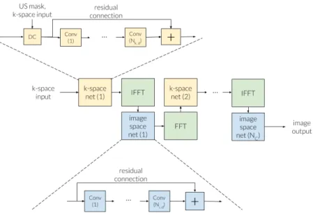
The second class of networks we introduce, we term cross-domain networks. The key intuitive idea is that they correct the data in both the k-space and the im-age space alternatively, using the Fourier transform to go from one space to the other. They are derived from the optimisation algorithms used to solve the op-timisation problems introduced before, using the idea of “unrolling” introduced in [30]. An illustration of this class of networks is presented in Figure 2.
Because these networks work directly on the input data (and not on a pri-marily reconstructed version of it), they need to handle complex-valued data. In particular, the classical deep learning frameworks (TensorFlow and Pytorch) do not feature the ability to perform complex convolutions off-the-shelf. The way convolution is performed in the original papers is therefore to concatenate the real and imaginary of the image (respectively the k-space), making it a 2-channel image, perform the series of convolutions, and have the output be a 2-channel image then transformed back in a complex image (respectively k-space).
prob-Figure 2: The common backbone between the Cascade net, the KIKI-net and the PD-net. US mask stands for under-sampling mask. DC stands for data consistency. (I)FFT stands for (Inverse) Fast Fourier Transform. Nk,d is the
number of convolution layers applied in the k-space. Ni,dis the number of
convo-lution layers applied in the image space. NC is the total number of alternations
between the k-space and the image-space. It is to be noted that in the case of PD-net, the data consistency step is not performed, the Fourier operators are performed with the original under-sampling mask, and a buffer is concatenated along with the current iteration to allow for some memory between iterations and learn the acceleration (in the k-space net -dual net- it is also concatenated with original k-space input). In the case of the Cascade net, Nk,d = 0, only the
data consistency is performed in the k-space. In the case of the KIKI-net, there is no residual connection in the k-space. However, the k-space nets and image space nets could potentially be any kind of image-to-image neural network.
Figure 3: Illustration of the Cascade-net from [10]. Here each Ci is a
con-volutional block of 64 filters (48 in our implementation) followed by a ReLU non-linearity, nd is the number of such convolutional blocks forming a
convo-lutional subnetwork between each data consistency layer DC, and nc is the
number of convolutional subnetworks.
Figure 4: Illustration of the KIKI-net from [9]. The KCNN and ICNN are convo-lutional neural networks composed of a number of convoconvo-lutional blocks varying between 5 and 25 (we implemented 25 blocks for both KCNN and ICNN), each followed by a ReLU non-linearity and featuring between 8 and 64 filters (we implemented 32 filters). For both the varying numbers, the supplementary ma-terial of [9] shows that the higher the better. The ICNN also features a residual connection.
lem (4). The idea is to replace the dictionary learning step by convolutional neural networks and still keep the data consistency step in the k-space. The optimisation algorithm is then unrolled to allow to perform back-propagation. [10] shows that we can perform back-propagation through the data consistency step (which is linear), and derive the corresponding Jacobian. The parameters used here for the implementation are the same as those in the original paper, except the number of filters which was decreased from 64 to 48 to fit on a single GPU. This network is illustrated in Figure 3.
The KIKI-net [9] is an extension of the Cascade-net where they additionally perform convolutions after the data consistency step in the k-space. The pa-rameters used here for the implementation are the same as those in the original paper. This network is illustrated in Figure 4.
Figure 5: Illustration of the PD-net from [8]. Here T denotes the measurement operator, which in our case is the under-sampled Fourier transform, T∗ its adjoint, g is the measurements, which in our case are the undersampled k-space measurements, and f0 and h0 are the initial guesses for the direct and
measurement spaces (the image and k-space in our case). The initial guesses are zero tensors. Because we transform complex-valued data into 2-channel real-valued data, the number of channels at the input and the output of the convolutional subnetworks are multiplied by 2 in our implementation.
MRI by [31], is based on the wavelet-based denoising (3), and in particular the resolution of the corresponding optimisation problem with the PDHG [22] algorithm. Here the algorithm is unrolled and the proximity operators (present in the general case of PDHG) are replaced by convolutional neural networks. For our implementation, for a fairer comparison with Cascade-net and the U-net, we used a ReLU non-linearity instead of a PReLU [32]. This network is illustrated in Figure 5.
3.4
Training
The training was done with the same parameters for all the networks. The opti-miser used was Adam [33], with a learning rate of 10−3 and default parameters of Keras (β1 = 0.9, β2 = 0.999, the exponential decay rates for the moment
estimates). The gradient norm was clipped to 1 to avoid the exploding gradient problems [34]. The batch size was 1 (i.e. one slice) for every network except the U-Net where the whole volume was used for each step. For all networks, to max-imise the efficiency of the training, the slices were selected in the 8 innermost slices of the volumes, because the outer slices do not have much signal. No early stopping or learning rate schedule was used (except for KIKI-net to allow for a stable training where we used the learning rate schedule proposed by the authors in the supporting information of [9]). The number of epochs used was 300 for all networks trained end-to-end. For the iterative training of the KIKI-net, the total number of epochs was 200 (50 per sub-training). Batch normalization was not used, however, in order to have the network learn more efficiently, a scaling of the input data was done. Both the k-space and the image were multiplied by
106for fastMRI and by 102for OASIS, because the k-space measurements had values of mean 10−7 (looking separately at the real and imaginary parts) for fastMRI and of mean 10−3for OASIS. Without this scaling operation, the train-ing proved to be impossible with bias in the convolutions and very inefficient without bias in the convolutions.
4
Data
4.1
Under-sampling
The under-sampling was done retrospectively using a Cartesian mask described in the data set paper [11], and an acceleration factor of 4 (i.e. only 25% of the k-space was kept). It contains a fully-sampled region in the lower frequencies, and randomly selects phase encoding lines in the higher frequencies.
It is to be noted that different under-sampling strategies exist in CS-MRI. Some of them are listed in [35], like for example spiral or radial. These strategies allow for a higher image quality while having the same acceleration factor or the same image quality with a higher acceleration factor. Typically, the spiral under-sampling scheme was designed to allow fast coronary imaging [36, 37]. These under-sampling strategies must take into account kinematic constraints (both physically and safety based), but also should also be with variable den-sity [35]. Recent works even try to optimize the under-sampling strategy under these kinematic constraints [38]. Others have tried to learn the under-sampling strategy in a supervised way. In [39], the under-sampling strategy is learned with a greedy optimisation. In [40], a gradient descent optimisation is used. Some approaches ([16, 41, 42] even try to learn jointly the optimal under-sampling strategy along with the reconstruction.
4.2
fastMRI
The data used for this benchmark is the emulated single-coil k-space data of the fastMRI dataset [11], along with the corresponding ground truth images. The acquisition was done with a 15-channel phased array coil, in Cartesian 2D Turbin Spin Echo (TSE). The pulse sequences were proton-density weighting, half with fat suppression, half without, some at 3.0 Teslas (T) others at 1.5 T. The sequence parameters were as follows: Echo train length 4, matrix size 320 × 320, in-plane resolution 0.5mm×0.5mm, slice thickness 3mm, no gap between slices. In total, there are 973 volumes (34, 742 slices) for the training subset and 199 volumes (7135 slices) for the validation subset.
Since the k-spaces are of different sizes, therefore resulting in images of different sizes, the outputs of the cross-domain networks were cropped to a central 320 × 320 region. For the U-net, the input of the network was cropped.
4.3
OASIS
The Open Access Series of Imaging Studies (OASIS) brain database [12] is a database including MRI scans of 1068 participants, yielding 2168 MR sessions. Of these 2168, we select only 2164 sessions which feature T1-weighted sequences. 1878 of these were acquired on a 3.0 T, 236 at 1.5 T and the remaining are undisclosed (50). The slice size is majorly 256 × 256, and sometimes 240 × 256 (rarely it can be some other sizes).The number of slices per scan is majorly 176, and sometimes 160 (rarely it can be smaller).
The data was then separated in a training and a validation set. The split was participant-based, that is a participant cannot have a scan in both sets. The split was of 90% for the training set and 10% for the validation set. We further reduced the training data to make it comparable to fastMRI, to 1000 scans randomly selected for the training subset and 200 scans randomly selected for the validation subset.
Contrarily to fastMRI, the OASIS data is available only in magnitude and therefore is only real-valued.The k-space is computed as the inverse Fourier transform of the magnitude image.
5
Results
5.1
Metrics
The metrics we used to benchmark the different networks are the following: • The Peak Signal-to-Noise Ratio (PSNR)
• The Structural SIMilarity index (SSIM) [43] • The number of trainable parameters in the network
• The runtime in seconds of the neural network on a single volume The PSNR is computed as follows, on whole magnitude volumes:
P SN R(x, ˆx) = 10 log10 max(x)
2 1
n
P
i,j,k(xi,j,k− ˆxi,j,k)2
!
(5)
where x is the ground truth volume, ˆx is the predicted volume (magnitude image), and n is the total number of points in the ground truth volume (same as the predicted volume). Since this metric compares very local differences it does not necessarily reflect the global visual comparison of the images. The SSIM was introduced in [43] exactly to take more structural differences or similarities between images into account. It is computed as in the original paper, per slice then averaged over the volume (the range however is computed volume-wise):
SSIM (x, ˆx) = (2µxµˆx+ c1)(2σxσxˆ+ c2)(covxˆx+ c3) (µ2
x+ µ2xˆ+ c1)(σx2+ σxˆ2+ c2)(σxσˆx+ c3)
where x is the ground truth slice, ˆx is the predicted slice, µi is the mean of i,
σi2 is the variance of i, covij is the covariance between i and j, c1 = (k1L)2,
c2 = (k2L)2, c3 = c22, L is the range of the values of the data (given because
computed over the whole volume), and k1= 0.01 and k2= 0.03.
While the 2 aforementioned metrics control the reconstruction quality, it is important to note that this is not the only factor to take into account when designing reconstruction techniques. Because the reconstruction has to happen fast enough for the MR physician to decide whether to re-conduct the exam or not, it is important for the proposed technique to have a reasonable recon-struction speed. For real-time MRI applications or dynamic MRI (e.g. cardiac imaging), it is even more important (for example in the context of monitoring surgical operations [44]). The runtimes were measured on a computer equipped with a single GPU Quadro P5000 with 16GB of RAM.
Concurrently, the number of parameters has to stay relatively low to allow the implementation on the different machines with potentially limited memory, which will probably need to have multiple models (for different contrasts, differ-ent organs or differdiffer-ent undersampling schemes including differdiffer-ent acceleration factors).
5.2
Quantitative results
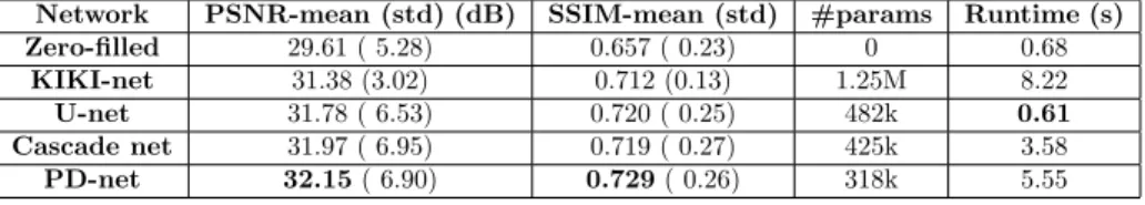
Table 1: Quantitative results for the fastMRI dataset. PSNR and SSIM mean and standard deviations are computed over the 200 validation volumes. Run-times are given for the reconstruction of a volume with 35 slices.
Network PSNR-mean (std) (dB) SSIM-mean (std) #params Runtime (s) Zero-filled 29.61 ( 5.28) 0.657 ( 0.23) 0 0.68
KIKI-net 31.38 (3.02) 0.712 (0.13) 1.25M 8.22 U-net 31.78 ( 6.53) 0.720 ( 0.25) 482k 0.61 Cascade net 31.97 ( 6.95) 0.719 ( 0.27) 425k 3.58 PD-net 32.15 ( 6.90) 0.729 ( 0.26) 318k 5.55 The quantitative results in Tables 1–4 show that the PD-net [8] outperforms its competitors in terms of image quality metrics but also has the least amount of trainable parameters. It it slightly slower than the Cascade-net [10] though
Table 2: Quantitative results for the fastMRI dataset with the Proton den-sity fat suppression (PDFS) contrast. PSNR and SSIM mean and standard deviations are computed over the 99 validation volumes. Runtimes are given for the reconstruction of a volume with 35 slices.
Network PSNR-mean (std) (dB) SSIM-mean (std) # params Runtime (s) Zero-filled 28.44 (2.62) 0.578 (0.095) 0 0.41
KIKI-net 29.57 (2.64) 0.6271 (0.10) 1.25M 8.88 Cascade-net 29.88 (2.82) 0.6251 (0.11) 425K 3.57 U-net 29.89 (2.74) 0.6334 (0.10) 482K 1.34 PD-net 30.06 (2.82) 0.6394 (0.10) 318K 5.38
Table 3: Quantitative results for the fastMRI dataset with the Proton den-sity (PD) contrast. PSNR and SSIM mean and standard deviations are com-puted over the 100 validation volumes. Runtimes are given for the reconstruc-tion of a volume with 40 slices.
Network PSNR-mean (std) (dB) SSIM-mean (std) # params Runtime (s) Zero-filled 30.63 (2.1) 0.727 (0.087) 0 0.52
KIKI-net 32.86 (2.4) 0.797 (0.082) 1.25M 11.83 U-net 33.64 (2.6) 0.807 (0.084) 482K 1.07 Cascade-net 33.98 (2.7) 0.811 (0.086) 425K 4.22 PD-net 34.2 (2.7) 0.818 (0.084) 318280 6.08
Table 4: Quantitative results for the OASIS dataset. PSNR and SSIM mean and standard deviations are computed over the 200 validation volumes. Run-times are given for the reconstruction of a volume with 32 slices.
Network PSNR-mean (std) (dB) SSIM-mean (std) # params Runtime (s) Zero-filled 26.11 (1.45) 0.672 (0.0307) 0 0.165
U-net 29.8 (1.39) 0.847 (0.0398) 482k 1.202 KIKI-net 30.08 (1.43) 0.853 (0.0336) 1.25M 3.567 Cascade-net 32.0 (1.731) 0.887 (0.0327) 425k 2.234 PD-net 33.22 (1.912) 0.910 (0.0358) 318k 2.758
which can be explained by its higher number of iterations, involving therefore more costly Fourier transform (inverse or direct) operations. These results hold true on the 2 data sets, fastMRI [11] and OASIS [12]. The only exception is that KIKI-net [9] is slightly better than the U-net [27] on the OASIS data set, but still far from the best performers. We can also note that the standard deviation of the image quality metrics is way higher in the fastMRI data set than in the OASIS data set. This higher standard deviation is explained by the fact that the 2 contrasts present in the fastMRI dataset, Proton Density with and without Fat Suprression (PD/PDFS), have widely different image metrics values. The standard deviations when we compute the metrics for each contrast separately are more in-line with the OASIS ones. The range of the image quality metrics is also much higher in the OASIS results.
5.3
Qualitative results
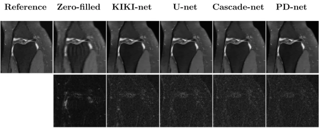
The qualitative results shown in Figures 6 – 7 confirm the quantitative ones on the image quality aspect. The PD-net [8] is much better at conserving the high-frequency parts of the original image, as can be seen when looking at the reconstruction error, which is quite flat over the whole image.
6
Discussion
In this work we only considered one scheme of under-sampling. However, it should be interesting to see if the performance obtained on one type of under-sampling generalizes to other types of under-under-sampling, especially if we do a
Reference Zero-filled KIKI-net U-net Cascade-net PD-net
Figure 6: Reconstruction results for a specific slice (16th slice of file1000196, part of the validation set). The first row represents the reconstruction using the different methods, while the second represents the absolute error when compared to the reference.
Reference Zero-filled KIKI-net U-net Cascade-net PD-net
Figure 7: Reconstruction results for a specific slice (15th slice of sub-OAS30367 ses-d3396 T1w.nii.gz, part of the validation set). The top row represents the reconstruction using the different methods, while the bottom row represents the absolute error when compared to the reference.
re-gridding step for non-Cartesian under-sampling schemes. On that specific point, the extension of the networks towards non-Cartesian sampling schemes is not easy because the data consistency cannot be performed in the same way, and the measurement space is no longer similar to an image (except if we re-grid). In a recent work [45], some of the authors of the Cascade-net [10] propose a way to extend their approach to the non-Cartesian case, using a re-gridding step. The PD-net [8] also has a straightforward implementation for the non-Cartesian case even without re-gridding, in what is called the learned Primal. In this case, the network in the k-space is just computing the difference (residual) between the current k-space measurements and the initial k-space measurements. Therefore there are no parameters to learn which alleviates the problem of how to learn them.
We also only considered a single-coil acquisition setting. As parallel imaging is primarily used in CS-MRI to allow higher image quality [3], it is important to see how these networks will behave in the multi-coil setting. The difficult part in the extension of these works to the multi-coil setting will be to understand how to best involve the sensitivity maps (or even not involve them [46]).
Regarding the networks themselves, the results seem to suggest that for cross-domain networks, the trade-off between a high number of iterations and a richer correction in a certain domain (by having deeper networks) is in fa-vor of having more iterations (i.e. alternating more between domains). It is however unclear how to best tackle the reconstruction in the k-space, since the convolutional networks make an shift invariance hypothesis which is not true in the Fourier space where the coefficients corresponding to the high frequencies should probably not be treated in the same way as with the low frequencies. This leaves room for improvement in the near future.
Finally, this work has not dealt with recent approaches involving adversarial training for MRI reconstruction networks [17, 47]. It would be very interesting to see how the adversarial training could improve each of the proposed networks.
References
[1] Z. Ramzi, P. Ciuciu, and J.-L. Starck. “Benchmarking proximal methods acceleration enhancements for CS-acquired MR image analysis reconstruc-tion”. In: SPARS 2019 - Signal Processing with Adaptive Sparse Structured Representations Workshop. Toulouse, France, July 2019.
[2] R. Smith-Bindman, D. L. Miglioretti, and E. B. Larson. “Rising use of diagnostic medical imaging in a large integrated health system”. In: Health affairs 27.6 (2008), pp. 1491–1502.
[3] P. B. Roemer et al. “The NMR phased array”. In: Magnetic resonance in medicine 16.2 (1990), pp. 192–225.
[4] M. Lustig, D. Donoho, and J. M. Pauly. “Sparse MRI: The Application of Compressed Sensing for Rapid MR Imaging”. In: Magnetic Resonance in Medicine (2007).
[5] NHS. NHS website. Accessed: 2019-12-05. url: https://www.nhs.uk/ conditions/mri-scan/what-happens/.
[6] A. S. Health. Clinical Appropriateness Guidelines: Advanced Imaging. 2017. url: https://www.aimspecialtyhealth.com/PDF/Guidelines/ 2017/Sept05/AIM_Guidelines.pdf (visited on 03/26/2019).
[7] B. Zhu et al. “Image reconstruction by domain-transform manifold learn-ing”. In: Nature 555.7697 (Mar. 2018), pp. 487–492.
[8] J. Adler and O. ¨Oktem. “Learned Primal-Dual Reconstruction”. In: IEEE Transactions on Medical Imaging 37.6 (2018), pp. 1322–1332.
[9] T. Eo et al. “KIKI-net: cross-domain convolutional neural networks for reconstructing undersampled magnetic resonance images”. In: Magnetic Resonance in Medicine 80.5 (2018), pp. 2188–2201.
[10] J. Schlemper et al. “A Deep Cascade of Convolutional Neural Networks for MR Image Reconstruction”. In: IEEE Transactions on Medical Imaging 37.2 (2018), pp. 491–503.
[11] J. Zbontar et al. “fastMRI: An open dataset and benchmarks for acceler-ated MRI”. In: arXiv preprint arXiv:1811.08839 (2018).
[12] P. J. LaMontagne et al. “OASIS-3: Longitudinal neuroimaging, clinical, and cognitive dataset for normal aging and Alzheimer’s disease”. In: Alzheimer’s & Dementia: The Journal of the Alzheimer’s Association 14.7 (2018), P1097.
[13] F. Chollet et al. Keras. https://keras.io. 2015.
[14] M. Abadi et al. TensorFlow: Large-Scale Machine Learning on Heteroge-neous Distributed Systems. Tech. rep. 2016.
[15] P. Virtue, S. X. Yu, and M. Lustig. “Better than real: Complex-valued neural nets for MRI fingerprinting”. In: Proceedings - International Con-ference on Image Processing, ICIP. Vol. 2017-Septe. 2018, pp. 3953–3957. [16] H. K. Aggarwal, M. P. Mani, and M. Jacob. “Modl-mussels: Model-based deep learning for multishot sensitivity-encoded diffusion mri”. In: IEEE Transactions on Medical Imaging 39.4 (2020), pp. 1268–1277.
[17] T. Minh Quan, T. Nguyen-Duc, and W.-K. Jeong. Compressed Sensing MRI Reconstruction using a Generative Adversarial Network with a Cyclic Loss. Tech. rep.
[18] Y. Yang et al. “Deep ADMM-net for compressive sensing MRI”. In: Neural Information Processing Systems. Nips. 2016, pp. 10–18.
[19] R. C. Petersen et al. “Alzheimer’s disease neuroimaging initiative (ADNI): clinical characterization”. In: Neurology 74.3 (2010), pp. 201–209. [20] J. P. Haldar. “Low-Rank Modeling of Local k-Space Neighborhoods
[21] L. Condat. “A Primal–Dual Splitting Method for Convex Optimization In-volving Lipschitzian, Proximable and Linear Composite Terms”. In: Jour-nal of Optimization Theory and Applications 158.2 (Aug. 2013), pp. 460– 479.
[22] A. Chambolle and T. Pock. “A First-Order Primal-Dual Algorithm for Convex Problems with Applications to Imaging”. In: (2011), pp. 120–145. [23] A. Beck and M. Teboulle. “A fast iterative shrinkage-thresholding algo-rithm for linear inverse problems”. In: SIAM Journal on Imaging Sciences 2.1 (2009), pp. 183–202.
[24] D. Kim and J. A. Fessler. “Adaptive restart of the optimized gradient method for convex optimization”. In: Journal of Optimization Theory and Applications 178.1 (2018), pp. 240–263.
[25] S. Ravishankar and Y. Bresler. “Magnetic Resonance Image Reconstruc-tion from Highly Undersampled K-Space Data Using DicReconstruc-tionary Learn-ing”. In: IEEE Transactions on Medical Imaging 30.5 (2011), pp. 1028– 1041.
[26] J. Caballero et al. “Dictionary learning and time sparsity for dynamic MR data reconstruction”. In: IEEE Transactions on Medical Imaging 33.4 (2014), pp. 979–994.
[27] O. Ronneberger, P. Fischer, and T. Brox. U-Net: Convolutional Networks for Biomedical Image Segmentation. Tech. rep.
[28] Y. Han, L. Sunwoo, and J. C. Ye. “k-space deep learning for accelerated MRI”. In: IEEE transactions on medical imaging (2019).
[29] C. Min Hyun et al. Deep learning for undersampled MRI reconstruction. Tech. rep. 2019.
[30] K. Gregor and Y. Lecun. “Learning Fast Approximations of Sparse Cod-ing”. In: (2010).
[31] J. Cheng et al. “Model learning: Primal dual networks for fast MR imag-ing”. In: International Conference on Medical Image Computing and Computer-Assisted Intervention. Springer. 2019, pp. 21–29.
[32] K. He et al. Delving Deep into Rectifiers: Surpassing Human-Level Per-formance on ImageNet Classification. Tech. rep.
[33] D. P. Kingma and J. Ba. Adam: A Method for Stochastic Optimization. 2014.
[34] R. Pascanu, T. Mikolov, and Y. Bengio. On the difficulty of training Re-current Neural Networks. 2012.
[35] N. Chauffert et al. “Variable density sampling with continuous trajecto-ries”. In: SIAM Journal on Imaging Sciences 7.4 (2014), pp. 1962–1992. [36] P. Irarrazabal and D. G. Nishimura. “Fast Three Dimensional Magnetic
Resonance Imaging”. In: Magnetic Resonance in Medicine 33.5 (1995), pp. 656–662.
[37] C. H. Meyer et al. “Fast Spiral Coronary Artery Imaging”. In: Magnetic Resonance in Medicine 28.2 (1992), pp. 202–213.
[38] C. Lazarus et al. “SPARKLING : variable-density k-space filling curves for accelerated T 2 * -weighted MRI”. In: Magnetic Resonance in Medicine (2019).
[39] T. Sanchez et al. “Scalable Learning-Based Sampling Optimization for Compressive Dynamic MRI”. In: ICASSP, IEEE International Conference on Acoustics, Speech and Signal Processing - Proceedings 2020-May.16066 (2020), pp. 8584–8588.
[40] F. Sherry et al. “Learning the sampling pattern for MRI”. In: IEEE Trans-actions on Medical Imaging (2020).
[41] Y. Wu, M. Rosca, and T. Lillicrap. “Deep Compressed Sensing”. In: In-ternational Conference on Machine Learning (ICML). 2019.
[42] T. Weiss and A. Bronstein. PILOT : Physics-Informed Learned Optimized Trajectories for Accelerated MRI. Tech. rep. 2019.
[43] Z. Wang et al. “Image Quality Assessment: From Error Visibility to Struc-tural Similarity”. In: IEEE TRANSACTIONS ON IMAGE PROCESS-ING 13.4 (2004).
[44] K. A. Horvath et al. “Real-time Magnetic Resonance Imaging Guidance for Cardiovascular Procedures”. In: Seminars in thoracic and cardiovascular surgery. Vol. 19. 4. 2007, pp. 330–335.
[45] J. Schlemper et al. “Nonuniform Variational Network: Deep Learning for Accelerated Nonuniform MR Image Reconstruction”. In: Proceedings of the International Conference on Medical Image Computing and Computer-Assisted Intervention. 2019, pp. 57–64.
[46] L. E. Gueddari et al. “Calibrationless oscar-based image reconstruction in compressed sensing parallel MRI”. In: ISBI 2019 - International Sympo-sium on Biomedical Imaging. 2019.
[47] P. L. Dragotti et al. “DAGAN: Deep De-Aliasing Generative Adversarial Networks for Fast Compressed Sensing MRI Reconstruction”. In: IEEE Transactions on Medical Imaging 37.6 (2017), pp. 1310–1321.
![Figure 1: Illustration of the U-net from [27]. In our case the output is not a segmentation map but a reconstructed image of the same size (we perform zero-padding to prevent decreasing sizes in convolutions).](https://thumb-eu.123doks.com/thumbv2/123doknet/13461057.411664/7.918.213.703.198.534/figure-illustration-segmentation-reconstructed-perform-padding-decreasing-convolutions.webp)
![Figure 4: Illustration of the KIKI-net from [9]. The KCNN and ICNN are convo- convo-lutional neural networks composed of a number of convoconvo-lutional blocks varying between 5 and 25 (we implemented 25 blocks for both KCNN and ICNN), each followed by a R](https://thumb-eu.123doks.com/thumbv2/123doknet/13461057.411664/9.918.212.707.455.591/illustration-lutional-networks-composed-convoconvo-lutional-implemented-followed.webp)
![Figure 5: Illustration of the PD-net from [8]. Here T denotes the measurement operator, which in our case is the under-sampled Fourier transform, T ∗ its adjoint, g is the measurements, which in our case are the undersampled k-space measurements, and f 0](https://thumb-eu.123doks.com/thumbv2/123doknet/13461057.411664/10.918.213.716.191.371/illustration-measurement-operator-fourier-transform-measurements-undersampled-measurements.webp)