HAL Id: hal-00418217
https://hal.archives-ouvertes.fr/hal-00418217
Submitted on 17 Jan 2014
Segmentation of vectorial image features using shape
gradients and information measures
Ariane Herbulot, Stéphanie Jehan-Besson, Stefan Duffner, Michel Barlaud,
Gilles Aubert
To cite this version:
Ariane Herbulot, Stéphanie Jehan-Besson, Stefan Duffner, Michel Barlaud, Gilles Aubert. Segmenta-tion of vectorial image features using shape gradients and informaSegmenta-tion measures. Journal of Mathe-matical Imaging and Vision, Springer Verlag, 2006, 25 (3), pp.365-386. �10.1007/s10851-006-6898-y�. �hal-00418217�
Gradients and Information Measures
Ariane Herbulot
Laboratoire I3S, CNRS-UNSA 2000, route des Lucioles 06903 Sophia Antipolis, France [email protected]
St´ephanie Jehan-Besson and Stefan Duffner∗ Laboratoire GREYC-Image
6 Bd Marechal Juin 14050 Caen, France. [email protected] Michel Barlaud
Laboratoire I3S, CNRS-UNSA 2000, route des Lucioles 06903 Sophia Antipolis, France [email protected]
Gilles Aubert
Laboratoire J.A. Dieudonn´e, CNRS-UNSA Parc Valrose
06108 Nice Cedex 2, France [email protected]
Abstract. In this paper, we propose to focus on the segmentation of vectorial features (e.g. vector fields or color intensity) using region-based active contours. We search for a domain that minimizes a criterion based on homogeneity measures of the vectorial features. We choose to evaluate, within each region to be segmented, the average quantity of information carried out by the vectorial features, namely the joint entropy of vector components. We do not make any assumption on the underlying distribution of joint probability density functions of vector components, and so we evaluate the entropy using non parametric probability density functions. A local shape minimizer is then obtained through the evolution of a deformable domain in the direction of the shape gradient.
The first contribution of this paper lies in the methodological approach used to differentiate such a criterion. This approach is mainly based on shape optimization tools. The second one is the extension of this method to vectorial data. We apply this segmentation method on color images for the segmentation of color homogeneous regions. We then focus on the segmentation of synthetic vector fields and show interesting results where motion vector fields may be separated using both their length and their direction. Then, optical flow is estimated in real video sequences and segmented using the proposed technique. This leads to promising results for the segmentation of moving video objects.
1. Introduction
The notion of entropy has first been introduced by Shannon (Shannon, 1948) and further developed in the information theory framework whose principles can be found in (Cover and Thomas, 1991). Information measures such as entropy or mutual information can be efficiently managed for image and video segmentation (Herbulot et al., 2004a) or medical image registration (Wells et al., 1996; Maes et al., 1997). As far as segmentation is concerned, a region may be characterized using the average quantity of information, namely the entropy, carried out by the intensity. We propose here to focus on the segmentation of vectorial images features. We can for example consider the color intensity or motion vectors. Our goal is to segment homogeneous fields of vectors by considering not only their length but also their direction. We then propose to minimize the joint entropy of vector components. We do not make any assumption on the underlying distribution of joint probability density functions (pdfs) of vector components, and so we evaluate the entropy using non parametric pdfs.
These information measures are embedded into a variational frame-work. We search for an optimal domain with regards to a global cri-terion including both region-based and boundary-based terms. A local shape minimizer of this criterion may be reached using deformable do-mains, namely region-based active contours. The basic idea is to obtain, from the derivation of the criterion, a Partial Differential Equation (PDE) that drives an initial region towards a local shape minimum of the error criterion. Classically, we propose to make it evolve in the direc-tion of a gradient. However, since the set of image regions, i.e. the set of regular open domains in Rn, does not have a structure of vector space,
we cannot apply gradient descent methods in a straightforward fashion. We propose to use shape gradients coming from shape optimization theory (Delfour and Zol´esio, 2001) to bear on the problem. Such an approach has been detailed in (Jehan-Besson et al., 2003; Aubert et al., 2003) and is here further developed for the minimization of information measures using non parametric probability distribution functions (pdfs) of image features following the work in (Herbulot et al., 2004a).
These theoretical results are then applied to the segmentation of homogeneous color regions such as the face in video sequences and to segmentation of motion vectors. In this second part, the goal is to segment different motions in a sequence of images notably the mo-tion of objects from the global background momo-tion. There are many practical applications for this type of problem, e.g. the cinematic post-production, video monitoring, tracking of objects or human beings, video coding and indexation e.g. MPEG-4 or MPEG-7. Variational
approaches and region-based active contours have proven to be efficient for motion segmentation. Some authors choose to minimize the image differences (Jehan-Besson et al., 2002), while other consider parametric models for each region (Cremers and Soatto, 2003). Another approach consists in using the length of the motion vectors (Ranchin and Dibos, 2004) or the dominant direction (Roy et al., 2006). In this paper we are able to consider both the length and the direction of motion vectors by using the joint entropy.
In the following section, we recall shape derivation principles that will then be applied to the derivation of region-dependent descriptors involving non parametric pdfs of image features. Such a derivation will be used to deduce the evolution equation of an active contour that will minimize information measures such as the entropy of a region. These theoretical tools will then be applied to segment coherent regions of color intensity. They will then be developed for the segmentation of motion vectors in both synthetical images and real images.
2. Region-based Active Contours using Shape derivation tools
In this chapter we address the problem of optimisation of region and boundary functionals by means of active contours. Having introduced the basic idea of active contours and the different approaches that exist so far, we then describe how to calculate the evolution equation using shape derivation tools and finally explain some implementation details, notably the level set method.
2.1. Problem Statement
Active contours are based on the idea of evolving an initial contour on an image towards the boundary of the object(s) of interest. Formally, for a 2D image, the evolution of a curve can be described as follows:
∂Γ(s, τ )
∂τ = F N = v with Γ(τ = 0) = Γ0. (1)
Γ0 is the initial curve, s the arc length, τ the evolution parameter
and N the inward normal vector of Γ(s, τ ). For τ → ∞ the curve should converge to the object boundary. The term F represents the velocity function of the curve and is usually derived from an energy functional J. The energy functionals that appeared first in literature were boundary-based. A classical example is J(Γ) = R
k(b) can depend on the gradient of the image (Kichenassamy et al.,
1996; Caselles et al., 1997).
Following the pioneer works of (Cohen et al., 1993; Ronfard, 1994), region based functionals have then been added in order to incorporate global information on the region to segment:
J(Ω) =
Z
Ωk(x, Ω) dx (2)
where the vector x represents the location of the pixel and k(x, Ω) the descriptor of the region Ω. This descriptor can depend on the region itself and is then called dependent. An example of such region-dependent descriptor is k(x, Ω) = (I(x) − µ)2, where µ represents the
mean of the intensity over the region Ω. This descriptor has been used by (Chan and Vese, 2001; Debreuve et al., 2001) for the segmentation of homogeneous regions.
Generally one uses a linear combination of region-based and contour-based terms in order to perform a segmentation task. A simple example is the segmentation into two regions Ωin and Ωout, which basically
cor-respond to objects and background. An appropriate energy functional for this task would be:
J(Ωin, Ωout, Γ) = Z Ωin kin(x, Ωin) dx+ Z Ωout kout(x, Ωout) dx+ Z Γ kb(x) ds (3) where kinis the descriptor for the object region, koutfor the background
region and kb the descriptor for the contour.
The choice of the descriptors is dependent on the application. In this article we propose to focus on information measures such as the joint entropy of vector components. Once this choice is made the terms have to be differentiated with respect to the geometry in order to calculate a velocity function that drives an initial contour towards a minimum. A detailed state of the art on region-based active contours can be found in (Jehan-Besson et al., 2003). Let us briefly note that some authors do not compute the theoretical expression of the velocity field but choose a deformation of the curve that will make the crite-rion decrease (Chesnaud et al., 1999). Other authors (Zhu and Yuille, 1996; Chan and Vese, 2001; Paragios and Deriche, 2002) compute the theoretical expression of the velocity vector from the Euler-Lagrange equations. The computation is performed in two main steps. First, region integrals representing region functionals are transformed into boundary integrals using the Green-Riemann theorem. Second, the corresponding Euler-Lagrange equations are derived, and used to define a dynamic scheme in order to make evolve the initial region. Another alternative is to keep the region formulation to compute the gradient
of the energy criterion with respect to the region instead of reducing region integrals to boundary integrals. In (Debreuve et al., 2001), the authors propose to compute the derivative of the criterion while taking into account the discontinuities across the contour. In (Jehan-Besson et al., 2001; Jehan-Besson et al., 2003) the computation of the evolution equation is achieved through shape derivation principles.
This computation becomes more difficult for region-dependent de-scriptors. It happens when statistical features of a region such as, for example, the mean or the variance of the intensity, are involved in the minimization. This case has been studied in (Chan and Vese, 2001; Debreuve et al., 2001; Jehan-Besson et al., 2001; Kim et al., 2002; Yezzi et al., 1999). In (Jehan-Besson et al., 2001; Jehan-Besson et al., 2003) the authors show that the minimization of functionals involving region-dependent features can induce additional terms in the evolution equation of the active contour that are important in practice. These additional terms are easily computed thanks to shape deriva-tion tools. In the following, we present shape derivaderiva-tion tools for the computation of the evolution equation.
2.2. Computation of the evolution equation using shape derivation tools
In order to obtain the evolution equation of the active contour ∂Γ(τ )∂τ that will lead to a minimum of the energy criterion J, it is necessary to differentiate the criterion. The criterion can contain contour-based and region-based terms as mentioned in equation (3). When calculating the evolution equation there are certain problems to solve. Firstly: with respect to which variable do we have to differentiate the criterion? As we are dealing with regular open domains in Rn that do not have the structure of vector spaces, it is difficult to compute the derivative and so the evolution equation. This problem can be tackled by the use of shape derivation tools (Delfour and Zol´esio, 2001) as detailed in (Aubert et al., 2003; Jehan-Besson et al., 2001; Jehan-Besson et al., 2003). Secondly the region-based terms show a double dependence, because the descriptor as well as the integration domain depend on the region. This has to be taken into account when calculating the evolution equation. To obtain the evolution equation three principal steps are performed:
1. Introduction of transformations
2. Derivation of the criterion using shape optimisation theorems 3. Computation of the evolution equation from the derivative
2.2.1. Introduction of transformations
The optimisation of the region functional (2) is difficult and the vari-ations of a domain must be clearly defined. Formally we introduce a mapping Tτ that transforms the initial domain Ω into the current
domain Ω(τ ). For a point x ∈ Ω, we denote:
x(τ ) = T (τ, x) with T (0, x) = x Ω(τ ) = T (τ, Ω) with T (0, Ω) = Ω.
Let us now define the velocity vector field V corresponding to T (τ ) as V(τ, x) = ∂T
∂τ(τ, x) ∀x ∈ Ω ∀τ ≥ 0. 2.2.2. Shape derivation tools
We now introduce two main definitions:
DEFINITION 1. The Eulerian derivative of Jr(Ω) =RΩk(x, Ω)dx in
the direction of V, noted dJr(Ω, V), is equal to:
dJr(Ω, V) = lim τ →0
Jr(Ω(τ )) − Jr(Ω)
τ if the limits exists.
DEFINITION 2. The shape derivative of k(x, Ω), noted ks(x, Ω, V ),
is equal to:
ks(x, Ω, V) = lim τ →0
k(x, Ω(τ )) − k(x, Ω) τ
if the limits exists.
The following theorem gives a general relation between the Eulerian derivative and the shape derivative for region-based terms.
THEOREM 1. Let Ω be a C1 domain in Rn and V a C1 vector
field. Let k be a function C1. The functional Jr(Ω) = R Ω
k(x, Ω) dx is differentiable and its Eulerian derivative in the direction of V is the following: dJr(Ω, V) = Z Ω ks(x, Ω, V)dx − Z ∂Ω k(x, Ω)(V · N)da
The proof can be found in (Sokolowski and Zol´esio, 1992; Delfour and Zol´esio, 2001).
2.2.3. Computation of the evolution equation for region-based terms Let us now consider the derivative of region-based terms. As we differ-entiate with respect to the region Ω, we have to distinguish the cases where the descriptors depend and do not depend on the region. 2.2.3.1. Region-independent descriptors: If a descriptor of a region-based term is not dependent on the region, the derivation is straigthfor-ward. Let Jr(Ω) =RΩk(x, Ω)dx be the criterion. Obviously k(x, Ω) =
k(x) and so ks = 0. Consequently the Eulerian derivative of Theorem
1 is reduced to:
dJr(Ω, V) = − Z
∂Ωk(x)(V · N) da (4)
and the evolution equation, respectively the velocity, can be calculated using the gradient descent method:
∂Γ(p, τ )
∂τ = k(x)N = v (5)
Γ(p, 0) = Γ0(p).
2.2.3.2. Region-dependent descriptors: Region-dependent descriptors of the form Jr(Ω) =RΩk(x, Ω)dx are more complicated to differentiate.
Using Theorem 1 one obtains a derivative of the following form: dJr(Ω, V) = − Z ∂Ω ¡ k(x, Ω) + A(x, Ω)¢ (V · N) da. (6)
A(x, Ω) is a term that comes from the region-dependence and so from the evaluation of the shape derivative ks. Jehan-Besson et al.
(Jehan-Besson et al., 2003; Aubert et al., 2003) describe a general framework for deriving some region-dependent descriptors based on statistical parameters.
2.2.3.3. Example: Let us consider a descriptor involving the mean of the intensity of the region:
k(x, Ω) = ϕ(I(x) − µ(Ω)) (7)
with ϕ a positive function of class C1 (Charbonnier et al., 1997). The criterion J is then given by:
J(Ω) =
Z
The Eulerian derivative of the criterion J(Ω) can be expressed as follows: dJr(Ω, V) = Z Ω− dµ dτϕ ′ (I(x) − µ(Ω)) dx − Z ∂Ωϕ(I(x) − µ(Ω))(V · N)da with ϕ′(r) = dϕdr.
The mean can be written using domain integrals : µ(Ω) = 1 |Ω| Z ΩI(x)dx = R ΩI(x)dx R Ωdx ,
and so, by applying again the shape derivative theorem, we get: dµ dτ = 1 |Ω|2 µ − Z ∂ΩI(x)(V · N)da. Z Ω dx + Z Ω I(x)dx. Z ∂Ω(V · N)da ¶ = 1 |Ω| Z ∂Ω(I(x) − µ(Ω))(V · N)da.
In this expression, we no longer have domain integrals. By replacing the derivative of µ in eq.(8), we obtain the following formulation:
dJr(Ω, V) = Z Ωϕ ′ (I(x) − µ(Ω)) Z ∂Ω I(x) − µ(Ω) |Ω| (V · N)da − Z ∂Ωϕ(I(x) − µ(Ω))(V · N)da.
The term A(x, Ω) from eq.(6) is given by: A(x, Ω) = ϕ′(I(x) − µ(Ω))
Z ∂Ω
I(x) − µ(Ω)
|Ω| .
By changing the order of integration in the derivative, we can compute the evolution equation of the active contour :
∂Γ(p, τ ) ∂τ = ³ ϕ(I(x) − µ(Ω)) − I(x) − µ(Ω) |Ω| Z Ω ϕ′(I(x) − µ(Ω))dx´N. (8) This example illustrates the derivation of a simple region-dependent descriptor involving parametric probability distribution functions (pdfs). In this report we get further interested in nonparametric pdfs as de-tailed in section 3.
2.2.4. Computation of the evolution equation for contour-based terms Contour based terms have the form Jb(Ω) =R∂Ωkb(x) da. Their
Eule-rian derivative in the direction vn = (V · N) is (Delfour and Zol´esio,
2001): dJb(Γ, vn) = Z ∂Ω ¡ ∇kb(x) · N − kb(x)κ¢(V · N) da. (9)
with N the unit inward normal of Γ, κ the mean curvature of Γ and da its area element. The evolution equation is consequently:
∂Γ(p, τ )
∂τ =
¡
kb(x)κ − ∇kb(x) · N¢N
Γ(p, 0) = Γ0(p). (10)
This result is the classical result found in (Caselles et al., 1997) using calculus of variations.
2.3. Implementation Using the Level Set Method
There are basically two approaches to implement active contours. The explicit approach uses an explicit parameterization of the contour, e.g. by B-splines (Precioso et al., 2005) or polygons, and the implicit ap-proach represents the curve by means of a function of higher dimension, e.g. the level set method (Osher and Sethian, 1988). In the following we are going to concentrate on the level set method, because among other advantages it implies the ability to change the topology.
The idea is to express the curve by means of a higher dimensional function U (x, τ ) in such a way that the zero level of U (x, τ ) represents the curve Γ(p, τ ). More formally we look for a function U : R2×R+→ R
such that:
Γ(p, τ ) = {x | U(x, τ) = 0}. (11)
An equivalent expression is:
U (Γ(p, τ ), τ ) = 0, ∀p ∈ [a, b], ∀τ ≥ 0. (12) U can be chosen as the signed distance function, i.e. the value U (x, τ ) represents the signed distance of the point x to the contour. We choose negative values inside the curve (region containing the objects) and positive values outside.
The normal vector N and the curvature κ can be directly derived from the level set function:
N= − ∇U
|∇U| and κ = div
µ
∇U |∇U|
This leads to the evolution equation: ∂U (τ )
∂τ = F |∇U|. (13)
The equation is only valid for U = 0 but it can be extended to the whole image domain ΩI if F is defined over the entire image. However
the signed distance function is not a solution to the extended PDE (13), see Gomes and Faugeras (Gomes and Faugeras, 2000). Therefore the function U has to be reinitialised so that it remains a distance function. When implementing the level set method it is useful to perform the calculations only over a narrow band enclosing the contour instead of the entire image. This reduces the time complexity of O(N2) to O(kN )
where N is the grid size.
Additionally a multiresolution technique can be applied in order to decrease calculation time, i.e. the contour evolution is performed on different resolutions starting from an image of reduced size and ending at the original image size. When passing to a higher resolution the final contour of the previous resolution serves as the initial contour of the current resolution.
3. Introduction of Descriptors based on information theory measures
We aim for a segmentation into regions with approximately homoge-neous statistical features. Many approaches use statistical measures like the mean or the variance of some feature(s) inside a region to formulate descriptors. Another approach based on information theory, notably on the entropy has been presented in (Kim et al., 2002; Herbulot et al., 2004a; Herbulot et al., 2004b). Indeed, the entropy concept designates the average quantity of information carried out by a feature. Intuitively the entropy represents some kind of diversity of a given feature. In this report we get further interested in computing the entropy without any assumption on the underlying distribution, i.e. using nonparametric pdfs. We first present general results for the minimization of func-tions of non parametric pdfs and we then apply these results for the minimization of the entropy and the conditional entropy.
3.1. Derivation of descriptors based on non parametric probability density functions
Let f (x) be the feature of interest and q(f (x), Ω) be the probability to have feature f (x) with x ∈ Ω. A general criterion can be defined as
follows: J(Ω) = Z Ω ϕ¡ q(f (x), Ω)¢ dx (14)
where ϕ is a function: R+→ R+of the probability, e.g. the entropy or the conditional entropy.
The probability distribution is estimated using the Parzen window method:
q(f (x), Ω) = 1 |Ω|
Z
ΩK(f (x) − f(ˆx)) dˆx (15)
where K is the Gaussian kernel of the estimation with 0-mean and Σ-covariance matrix and |Ω| the shape area. The kernel of a vector f = [f1, f2, .., fn]T is:
K(f ) = 1
(2π)n/2|Σ|1/2 exp ³
−12fTΣ−1f´.
In general, the covariance Σ depends on the number of samples, but in our case, the number of pixels in a region does not change a lot during the segmentation process. The computation is done for a fixed variance. See Appendix(B) for the computation with a variance depending on the number of pixels of the region Ω.
This criterion defined in (14) is now differentiated using the shape gradient theorem (Theorem 1). The Eulerian derivative of (14) in the direction V is then given by :
dJr(Ω, V) = Z Ω ϕs¡q(f (x), Ω), V¢dx− Z ∂Ω ϕ¡ q(f (s), Ω)¢ (V·N) ds (16) where N is the unit inward normal of the curve and ϕs is the shape
derivative of ϕ in the direction V.
ϕs¡q(f (x), Ω), V¢= ϕ′(q(f (x), Ω))qs(f (x), Ω, V)
with qs the Eulerian derivative of q in the direction V. We apply the
shape gradient theorem on q: qs(f (x), Ω, V) = 1 |Ω|2 Z ∂Ω(V · N) ds Z ΩK(f (x) − f(ˆ x)) dˆx − 1 |Ω| Z ∂ΩK(f (x) − f(s))(V · N) ds.
So the shape derivative of ϕ is: ϕs¡q(f (x), Ω), V¢= 1 |Ω| Z ∂Ωϕ ′¡ q(f (x), Ω)¢h q(f (x), Ω) − K¡ f(x) − f(s)¢i (V · N) ds
where ϕ′(q) represents the derivative of ϕ with respect to q. We can
then deduce the evolution equation of the active contour that leads J to a minimum: ∂Γ(s, τ ) ∂τ = ϕ ¡ q(f (ˆx), Ω)¢ N (17) − 1 |Ω| ·Z Ω ¡ q(f (x), Ω) − K¡ f(x) − f(ˆx)¢¢ ϕ′¡ q(f (x), Ω)¢ dx ¸ N with ˆx= Γ(s, τ ).
3.2. Minimization of the joint entropy for vectorial image features
The entropy represents the average quantity of information carried out by a feature, we may then minimize such a quantity for the segmen-tation of homogeneous regions. In this article, we are more particu-larly interested by the joint entropy of vectorial image features f (x) = [f1(x), f2(x)..., fn(x)]T. We treat f as an observation of a random vector
denoted by F. The continuous joint entropy can be expressed by: H(F, Ω) = 1 |Ω| Z Ω− ln q(f(x), Ω) dx (18) = 1 |Ω| Z Ω− ln q(f1 (x), f2(x), .., fn(x), Ω) dx
where q(f (x), Ω) represents the joint probability density function of the components of the vectorial feature f (x).
This energy can be written by: H(F, Ω) = 1
|Ω|
Z Ω
ϕ(q(f (ˆx), Ω)) dx (19)
with ϕ(q) = − ln q. Using the derivation scheme presented above, we can calculate the evolution equation:
∂Γ(s, τ ) ∂τ = − 1 |Ω|ln q(f (ˆx), Ω)N − 1 |Ω| · H(F, Ω) + 1 |Ω| Z Ω K(f (x) − f(ˆx)) q(f (x), Ω) dx − 1 ¸ N.
3.3. Application to region competition
In the experiments, we use a competition between the object region Ωin and the background region Ωout. These regions share the same
boundary Γ and we look for the regions that minimize the following criterion:
J(Ωin, Ωout, Γ) = H(F, Ωin) + H(F, Ωout) + Z
Γ
λds (20)
where λ is a regularization parameter.
Let us rewrite the definition (18) for the regions Ωin and Ωout:
H(F, Ωin) = 1 |Ωin| Z Ωin − ln q(f(x), Ωin)dx H(F, Ωout) = 1 |Ωout| Z Ωout − ln q(f(x), Ωout)dx.
By using the derivation tool presented in the previous section, we obtain the evolution equation of the active contour:
∂Γ(s, τ ) ∂τ = " − 1 |Ωin| ln q(f (ˆx), Ωin) (21) − 1 |Ωin| · H(F, Ωin) + 1 |Ωin| Z Ωin K(f (x) − f(ˆx)) q(f (x), Ωin) dx − 1 ¸ + 1 |Ωout| ln q(f (ˆx), Ωout) + 1 |Ωout| · H(F, Ωout) + 1 |Ωout| Z Ωout K(f (x) − f(ˆx)) q(f (x), Ωout) dx − 1 ¸ + λ.κ # N
where κ is the curvature of the curve Γ.
3.4. Minimization of the conditional entropy
When working with two regions Ωin and Ωout one can also use the
following criterion :
HC(Ωin, Ωout) = H(F, Ωin) · |Ωin| + H(F, Ωout) · |Ωout|. (22)
This criterion is based on a maximization of the mutual information between the feature f (x) and the label L(x) (Herbulot et al., 2004b; Kim et al., 2002), where L(x) maps a point x either to the object or the background label. It corresponds to the conditional entropy between the feature f (x) and the label L(x).
By performing the same procedure as in the last section we can cal-culate the Eulerian derivative in the direction V of J(Ω) = H(F, Ω) |Ω|: dJr(Ω, V) = Z ∂Ω h −1 + 1 |Ω| Z Ω K(f (x) − f(ˆx) q(f (x), Ω) dx + ln q(f (x), Ω) i (V · N) ds. This gives us the following evolution equation for the criterion (22): ∂Γ(s, τ ) ∂τ = h − 1 |Ωin| Z Ωin K(f (x) − f(ˆx) q(f (x), Ωin) dx − ln q(f(x), Ωin ) + 1 |Ωout| Z Ωout K(f (x) − f(ˆx) q(f (x), Ωout) dx + ln q(f (x), Ωout) i N. This gives an alternative proof to the result found in (Kim et al., 2002). However, the framework proposed in this paper allow us to consider any descriptor that can be written as a function of a non parametric pdf (e.g. distance functions). Derivation can also be easily performed for a kernel depending on the region Ω (see Appendix B). Note that a comparison between our method and calculus of variations has been given in (Aubert et al., 2003).
4. Segmentation of Color Images
Until now the feature(s) f (x) which can be used in our entropy-based energy criteria have not been specified. We can first choose f (x) to be two or more components of the intensity for the segmentation of color homogeneous regions, i.e. f (x) = [I1(x), .., In(x)]T.
In these experiments we consider two components of the intensity, i.e. f (x) = [I1(x), I2(x)]T and we use the joint entropy between the two
components I1and I2, H(Ω) = |Ω|1 RΩ− ln q(I1(x), I2(x), Ω) dx. We test
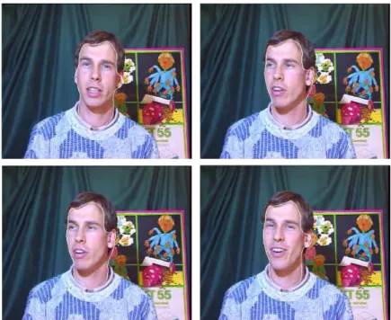
our algorithm on the video sequence Erik for the face segmentation. The Figure 1 shows the evolution of the curve, the histogram of the object and the Figure 2 the histogram of the background during the segmentation algorithm on a frame while the Figure 3 the evolution of the segmented region through a sequence. These results show the accuracy of the method for segmentation of homogeneous regions using intensity-based criterion.
5. Segmentation of Motion Vectors
We can also consider the motion vector coordinates as image features: f(x) = [u, v]T. Therefore we here consider a combination of two features and thus the probability q represents a joint probability and the entropy is a joint entropy, H(F, Ω) = |Ω|1 R
Ω− ln q(u(x), v(x), Ω) dx. Using such
an approach, we consider not only the length of the motion but also the motion direction as can be shown in the following synthetical examples. 5.1. Results on synthetic images
In the following some segmentation examples on synthetic motion fields are shown using region-based active contours and descriptors based on the conditional entropy. In order to incorporate not only the length of the motion but also the motion direction in the descriptors the 2-dimensional vector coordinates (u, v) are used.
The following diagrams show only every 10th vector of the motion fields. For the sake of clarity they have also been lengthened by factor 8. Note that the start point of the arrow is plotted over the point to which the velocity vector is related to.
The first example shows a rectangle moving rightwards on a back-ground moving leftwards (Fig. 4.a). The vectors of the rectangle and the background have the same length, so the vector length would not gives us a discriminative feature in this case. As we take into account the direction as well the rectangle can be segmented correctly from the background. Figure 4 shows the segmentation result of this example.
In the second example three rectangles of different size and motion are placed over a moving background (Fig. 5.a). Figure 5 illustrates the segmentation result. A small rectangle traversing the three different motion fields is chosen as initial contour so it has to extend at some locations and to shrink at other locations. Also at some point of time it changes its topology, i.e. it has to split. The evolution of the respective histograms is illustrated in Figure 6. In the left column three samples of the background histogram and in the right column three corresponding samples of the object histogram are depicted. Clearly the peak at (0, 1) corresponding to the background motion disappears gradually in the object histograms whereas in the background histogram it remains the only peak. This shows that our approach manages also to segment several objects with a completely different motion provided that the background motion is homogeneous.
The last example shows an enlarging disc over a background moving rightwards (Fig. 7.a). Here the motion vectors of the object point in nearly every direction. The length of the vectors is also not
homoge-neous inside the object. Nevertheless our method is able to segment properly the disc from the background because background motion is homogeneous. Figure 7 illustrates the result.
5.2. Motion Estimation on real sequences
So far we have only been investigating synthetic examples of motion fields. In order to segment real world image sequences we now have to estimate the motion between consecutive images. To this end we calculate the optical flow between consecutive pairs of images. Note that we can use any other accurate method of motion estimation as input of our segmentation algorithm.
5.2.1. Optical Flow
In the following an image sequence is denoted as I(x, y, t) where (x, y) represents the location in an image domain Ω and t the time. One way of estimating the motion in an image sequence is to calculate the optical flow, i.e. to calculate for each pixel a motion vector (u, v)T. The basic assumption for this calculation is that corresponding features maintain their intensity over time. This can be expressed in the optic flow constraint (OFC) equation:
∂I ∂xu + ∂I ∂yv + ∂I ∂t = 0 (23)
Solving this equation represents an ill-posed problem and requires a second constraint which ensures that the optical flow varies smoothly in space. We search for the optical flow (u, v) which minimizes the following functional: E(u, v) := Z Ω Ã µ∂I ∂xu + ∂I ∂yv + ∂I ∂t ¶2 + α Ψ³|∇u|2+ |∇v|2´ ! dx dy (24) where Ψ is an increasing differentiable function, ∇ := (∂x, ∂y)T the
2D nabla operator and α is a regularization parameter. It satisfies necessarily the Euler equations:
0 = ∇ ·³Ψ′(|∇u|2+ |∇v|2)∇u´− 1 α ∂I ∂x µ∂I ∂xu + ∂I ∂yv + ∂I ∂t ¶ (25) 0 = ∇ ·³Ψ′(|∇u|2+ |∇v|2)∇v´− 1 α ∂I ∂y µ∂I ∂xu + ∂I ∂yv + ∂I ∂t ¶ (26) where Ψ′ denotes the derivative of Ψ and ∇ ·¡a
b ¢
A solution to this can be obtained by calculating the steady-state of the diffusion-reaction process:
uk = ∇ · ³ Ψ′(|∇u|2+ |∇v|2)∇u´− 1 α ∂I ∂x µ∂I ∂xu + ∂I ∂yv + ∂I ∂t ¶ (27) vk = ∇ · ³ Ψ′(|∇u|2+ |∇v|2)∇v´− 1 α ∂I ∂y µ∂I ∂xu + ∂I ∂yv + ∂I ∂t ¶ (28) where k is the diffusion time and for k → ∞, the solution (u, v) represents a minimum of E(u, v).
The choice of the function Ψ influences substantially the regulariza-tion process and therefore the results of the moregulariza-tion estimaregulariza-tion. We choose the function that has been considered by Schn¨orr (Schn¨orr, 1994) and Weickert (Weickert, 1998):
Ψ(s2) = λ2q1 + s2/λ2 (29)
The parameter λ is a positive constant which serves as a contrast parameter see (Weickert, 1998).
The optical flow calculation can be implemented by an iterative approach using the equations (27) and (28). This gives the following for u and v at the iteration k + 1 at any position:
uk+1 = uk+ ∆k · ∇ ·¡ Ψ′(s)∇uk¢− 1 α ∂I ∂x µ∂I ∂xuk+ ∂I ∂yvk+ ∂I ∂t ¶¸ vk+1 = vk+ ∆k · ∇ ·¡ Ψ′(s)∇vk¢− 1 α ∂I ∂y µ∂I ∂xuk+ ∂I ∂yvk+ ∂I ∂t ¶¸
where s = |∇uk|2+|∇vk|2and ∆k is the step size. We simply start with
a flow field of zero-vectors and iteratively adjust the motion vectors for every pixel of the image until a certain convergence criterion has been reached. The convergence criterion is usually based on the difference of the energy functional to minimize between two iterations.
One practical problem that arises when estimating the optical flow is that larger movements were not sufficiently approximated, i.e. the algorithm gets stuck in local minima. In fact this happens when move-ments are larger than the size of the mask used for the approximation of the gradient. To overcome this a multiresolution procedure according to M´emin and P´erez (M´emin and P´erez, 1998) was implemented. That means that optical flow calculation is started on an image with coarser (downsampled) resolution Ij and continued by increasing (doubling)
the resolution step by step until the size of the original image I0 (j ranges from J to 0 where J represents the coarsest and 0 the finest resolution). At each resolution the motion vectors of the previous step
uj−1 are projected onto the new resolution (uj) and only the
differ-ences duj are calculated, i.e. the existing estimation is refined. The projection (subsequently denoted T ) can be a duplication or a bilinear interpolation.
Consequently the energy functional (24) becomes the following:
E(u, v) := Z Ω µµ ∇ ˜Ij· duj+I˜j t ¶2 + αΨ³|∇(T uj+1+ duj)|2+ |∇(T vj+1+ dvj)|2´ ¶ dx dy (30) where ˜Ij = Ij(x − T uj+1, t) and I˜j t = Ij(x, t + 1) − Ij(x − T uj+1, t).
The Multiresolution approach can also help to avoid holes in the tion field of homogeneous zones, i.e. where |∇I| is low. That means mo-tion fields of moving objects containing homogeneous zones are better filled while also rendering their boundaries more blurry.
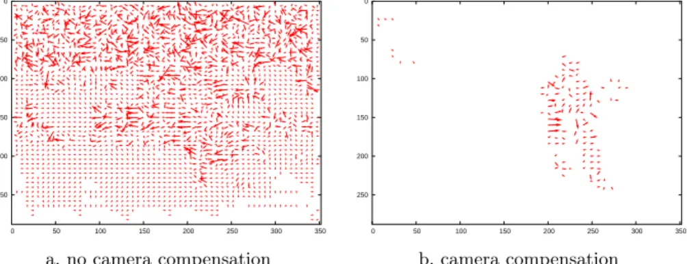
Object motion in image sequences is difficult to estimate if the se-quences come from a mobile camera. Much better results are achieved by compensating the camera motion, i.e. by estimating the global mo-tion. See Annexe.(A) for details.
5.3. Results on Real Sequences
Let us now apply the active contour segmentation method on the op-tical flow motion fields. The following results are all obtained using descriptors based on the conditional entropy (see eqn. 22). We used two competitive regions Ωin (object) and Ωout (background) in such a
way that the entropy of both regions will be minimized. Moreover a contour-based descriptor is used for regularisation to obtain smoother contours.
The optical flow as well as the active contour are calculated on two different resolutions. The features that have been used are the vector length |u| and the vector coordinates (u, v). The feature pair of vector length and direction did not lead to satisfying results. The estimation of the angle of the direction is prone to errors.
Figure 10 shows the final active contour of the ’tennis player’ se-quence using the motion vector length as the segmentation feature (f (x) = |u|). It can be remarked that one foot of the tennis player has not been segmented properly. This is simply because it does not move with respect to the two consecutive images that have been used. Clearly, as only features that are based on the optical flow have been used in the descriptors, objects that don’t move are not segmented.
The irregularities in the curve are mainly due to inconsistencies in the optical flow estimation. It would probably be useful to apply a vectorial regularization in order to take into account that the data are vectors and not scalar data. Moreover the little gap between the curve and the right border of the object is caused by erroneous motion detection of the optical flow method at zones that have been hidden (occlusion problem).
Figure 11 shows the final contour when using the entropy of the motion vector coordinates (u, v) instead of their length. Figure 12 shows the evolution of the respective histograms. The values are quantized using a 20 by 20 grid, however only the significant parts are displayed for the sake of clarity. These results are similar to those using the vector length.
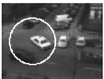
Figure 14 shows the segmentation results of the ’taxi’ sequence. Figure 13 illustrates the respective motion field. Here only taking the length of vectors does not lead to satisfying results especially with the car at the bottom left whereas taking (u, v) as segmentation feature yields much better contours for the respective objects.
6. Conclusion
In this article, we propose a method of images and video segmentation based on the minimization of a criterion. This criterion includes func-tions of images features such as the entropy or the conditional entropy. We relax the assumption of parametric distributions for these images features by using a Parzen estimation.
Our first contribution is to use the methodological approach of the shape gradient to derive the criterion. Second, we extend the method to vectorial data. Third we can easily take into account a kernel depending on the region in the Parzen estimator.
Experimental results show the accuracy of the presented method both on segmentation of color images and on segmentation of optical flow for moving objects in video sequences.
References
Aubert, G., M. Barlaud, O. Faugeras, and S. Jehan-Besson: 2003, ‘Image Segmenta-tion Using Active Contours: Calculus of VariaSegmenta-tions or Shape Gradients ?’. SIAM Applied Mathematics 63(6), 2128–2154.
Caselles, V., R. Kimmel, and G. Sapiro: 1997, ‘Geodesic active contours’. Interna-tional Journal of Computer Vision 22(1), 61–79.
Chan, T. and L. Vese: 2001, ‘Active contours without edges’. IEEE Transactions on Image Processing 10(2), 266–277.
Charbonnier, P., L. Blanc-F´eraud, G. Aubert, and M. Barlaud: 1997, ‘Deterministic edge-preserving regularization in computed imaging’. IEEE Transactions on Image Processing 6(2), 298–311.
Chesnaud, C., P. R´efr´egier, and V. Boulet: 1999, ‘Statistical region snake-based segmentation adapted to different physical noise models’. IEEE Transactions on Pattern Analysis and Machine Intelligence 21, 1145–1156.
Cohen, L., E. Bardinet, and N. Ayache: 1993, ‘Surface reconstruction using active contour models’. In: SPIE Conf. on Geometric Methods in Comp. Vis. San Diego.
Cover, T. and J. Thomas: 1991, Elements of Information Theory. Wiley-Interscience. Cremers, D. and S. Soatto: 2003, ‘Variational Space-Time Motion Segmentation’.
In: IEEE Int. Conf. on Computer Vision, Vol. 2. pp. 886–892.
Debreuve, E., M. Barlaud, G. Aubert, and J. Darcourt: 2001, ‘Space time segmenta-tion using level set active contours applied to myocardial gated SPECT’. IEEE Transactions on Medical Imaging 20(7), 643–659.
Delfour, M. and J. Zol´esio: 2001, Shape and geometries. Advances in Design and Control, SIAM.
Geman, S. and D. Mc Lure: 1985, ‘Bayesian image analysis: an application to single photon emission tomography’. In: Proc. Statist. Comput. Sect.
Gomes, J. and O. Faugeras: 2000, ‘Reconciling distance functions and level sets’. Journal of Visual Communication and Image Representation 11, 209–223. Herbulot, A., S. Jehan-Besson, M. Barlaud, and G. Aubert: 2004a, ‘Shape gradient
for image segmentation using information theory’. In: International Conference on Acoustics, Speech and Signal Processing. Montreal.
Herbulot, A., S. Jehan-Besson, M. Barlaud, and G. Aubert: 2004b, ‘Shape Gra-dient for Multi-Modal Image Segmentation Using Mutual Information’. In: International Conference on Image Processing. Singapore.
Jehan-Besson, S., M. Barlaud, and G. Aubert: 2001, ‘Video object segmentation using eulerian region-based active contours’. In: International Conference on Computer Vision. Vancouver, Canada.
Jehan-Besson, S., M. Barlaud, and G. Aubert: 2002, ‘A 3-Step algorithm using region-based active contours for video objects detection’. EURASIP Journal on Applied Signal Processing, Special issue on Image Analysis for Multimedia Interactive Services 2002(6), 572–581.
Jehan-Besson, S., M. Barlaud, and G. Aubert: 2003, ‘DREAM2S: Deformable
Re-gions driven by an Eulerian Accurate Minimization Method for image and video segmentation’. International Journal of Computer Vision (53), 45–70.
Kichenassamy, S., A. Kumar, P. J. Olver, A. Tannenbaum, and A. Yezzi: 1996, ‘Conformal Curvature Flows: From Phase Transitions to Active Vision’. Archive for Rational Mechanics and Analysis 134(3), 275–301.
Kim, J., J. Fisher III, A. Yezzi Jr., M. Cetin, and A. Willsky: 2002, ‘Nonpara-metric Methods for Image Segmentation Using Information Theory and Curve Evolution’. In: International Conference on Image Processing.
Maes, F., A. Collignon, D. Vandermeulen, G. Marchal, and P. Suetens: 1997, ‘Mul-timodality image registration by maximization of mutual information’. IEEE Transactions on Medical Imaging 16(2).
M´emin, E. and P. P´erez: 1998, ‘Dense Estimation and object-based segmentation of the optical flow with robust techniques’. IEEE Transactions on Image Processing 7(5), 703–718.
Odobez, J. and P. Bouthemy: 1995, ‘Robust multiresolution estimation of parametric motion models’. Journal of Visual Communication and Image Representation 6(4), 348–365.
Osher, S. and J. Sethian: 1988, ‘Fronts propagating with curvature-dependent speed: Algorithms based on Hamilton-Jacobi Formulation’. Journal of Computational Physics 79, 12–49.
Paragios, N. and R. Deriche: 2002, ‘Geodesic Active Regions: A new Paradigm to deal with frame partition Problems in Computer vision’. Journal of Visual Communication and Image Representation 13, 249–268.
Precioso, F., M. Barlaud, T. Blu, and M. Unser: to appear, 2005, ‘Robust Real-time Segmentation of Images and Videos using a Smoothing-spline Snake-based Algorithm’. IEEE Transactions on Image Processing.
Ranchin, F. and F. Dibos: 2004, ‘Moving Objects Segmentation Using Optical Flow Estimation’. In: Workshop on Mathematics and Image Analysis. Paris.
Ronfard, R.: 1994, ‘Region-based strategies for active contour models’. International Journal of Computer Vision 13(2), 229–251.
Roy, T., E. Debreuve, M. Barlaud, and G. Aubert: 2006, ‘Segmentation of a vector field: Dominant parameter and shape otimization’. Journal of Mathematical Imaging and Vision (In Press).
Schn¨orr, C.: 1994, ‘Segmentation of visual motion by minimizing convex non-quadratic functionals’. In: Proc. 12th Int. Conf. Pattern Recognition, Vol. A. Jerusalem, pp. 661–663, IEEE Computer Society Press, Los Alamitos.
Shannon, C.: 1948, ‘A mathematical theory of communication’. Bell Sys. Tech. J. 27, 379–423.
Sokolowski, J. and J. Zol´esio: 1992, Introduction to shape optimization, Vol. 16 of Springer series in computational mathematics. Springer-Verlag.
Weickert, J.: 1998, ‘On discontinuity-preserving optic flow’. In: Proc. Computer Vision and Mobile Robotics Workshop, Santorini. pp. 115–122.
Wells, W., P. Viola, H. Atsumi, S. Nakajima, and R. Kikinis: 1996, ‘Multi-modal volume registration by maximization of mutual information’. Medical Image Analysis 1(1), 35–51.
Yezzi, A., A. Tsai, and A. Willsky: 1999, ‘A statistical approach to snakes for bimodal and trimodal imagery’. In: Int. Conference on Image Processing. Kobe Japan. Zhu, S. and A. Yuille: 1996, ‘Region competition: unifying snakes, region growing,
and Bayes/MDL for multiband image segmentation’. IEEE Transactions on Pattern Analysis and Machine Intelligence 18, 884–900.
Appendix
A. Compensation of Camera Motion
Global motion estimation is often based on a parametric model. In our case this is a 6 parameter affine model and it is estimated using two consecutive images of a sequence (Odobez and Bouthemy, 1995; Jehan-Besson et al., 2002). The basic assumption we make is that the camera motion is dominant in these images, i.e. we assume that the size of the moving objects in the sequence is not too large with respect to the background.
The apparent motion wn(x) of a point x = [x, y]T in the 2D plane
between two images In−1 and Inis thus modeled by:
wn(x) = Anx+ tn= µ an 11 an12 an21 an22 ¶ µ x y ¶ + µ tn 1 tn2 ¶ . (31)
In order to estimate the parameters of the model the ”Block Match-ing” technique is applied. The principle of this method is to partition the current image into blocks and for each block to find the motion vector un = [dxn, dyn]T so that it corresponds to the respective block
in the preceding (or subsequent) image.
Using this estimation of movement we seek for the 6 parameters that minimize the following criterion:
G(An, tn) = X x∈ΩI
ϕ(|un(x) − Anx− tn|). (32)
The function ϕ eliminates outliers mainly due to object movement and is chosen as the estimator of Geman and McLure (Geman and Mc Lure, 1985).
Using the half-quadratic theorem (Charbonnier et al., 1997; Geman and Mc Lure, 1985) the minimization problem can be equivalently formulated as: (An, tn) = arg min (An,tn) X ΩI wrr2 (33) where r = |un− Anx− tn| and wr = ϕ ′(r) 2r .
The objective is to estimate the 6 affine model parameters with respect to two consecutive images, In−1 and In, and then to apply the
corresponding affine transformation on image In−1. This will create a
compensated image Icomp in such a way that the background remains
more or less fix between Icomp and In. Figure B illustrates this by
means of an example. The grey level represents the difference of the pixel intensity.
Figure 9 shows the effect of camera motion compensation in context with optical flow estimation. Without camera motion compensation it seems impossible to segment the tennis player from the background. This is due to the fact that the motion of homogeneous zones like the green tennis court are not estimated correctly.
B. Computation of the derivative of the pdf when the variance of the kernel depends on the number of pixels
of the region
Now, we rather consider the following estimator: q(f (x), Ω) = 1 h1p|Ω| Z Ω K µ (f (x) − f(ˆx))q|Ω| ¶ )dˆx. (34) In this case, the domain derivative of q is the following:
q′r(f (x), Ω, V) = 1 2|Ω| Z ∂Ω q(f (x), Ω)(V · N)ds + 1 h1p|Ω| Z ∂Ω M (f (x), Ω) − K µ (f (x) − f(s))q|Ω| ¶ (V · N)ds where: M (f (x), Ω) = Z Ω −(f(x) − f(ˆx)) 2p |Ω| K ′µ (f (x) − f(ˆx))q|Ω| ¶ dˆx. (35) Proof : Let us denote: G(Ω) = 1 h1p|Ω|
with h1 a normalization parameter. We can easily find that :
dGr(Ω, V) = 1 2 h1|Ω|3/2 Z ∂Ω (V · N)ds. Let us now denote:
H(f (x), Ω) = Z ΩK µ (f (x) − f(ˆx))q|Ω| ¶ )dˆx, (36) we find that : Hr′(f (x), Ω, V) = Z Ω −(f(x) − f(ˆx)) 2p |Ω| Z ∂Ω (V · N)ds K′ ³ (f (x) − f(ˆx))√Ω´dˆx − Z ∂Ω K µ (f (x) − f(s))q|Ω| ¶ (V · N)ds. This leads to:
Hr′(f (x), Ω, V) = Z ∂Ω µ M (f (x), Ω) − K µ (f (x) − f(s))q|Ω| ¶¶ (V · N)ds,
where we note: M (f (x), Ω) = Z Ω −(f(x) − f(ˆx)) 2p |Ω| K ′µ(f (x) − f(ˆx))q|Ω|¶dˆx. (37)
Let us now compute the shape derivative of q, we have :
q′r(f (x), Ω, V) = Hr′(F, Ω, V) G(Ω) + H(F), Ω) dGr(Ω, V). (38) And so : q′r(f (x), Ω, V) = 1 2|Ω| Z ∂Ω q(f (x), Ω)(V · N)ds + 1 h1p|Ω| Z ∂Ω M (f (x), Ω) − K µ (f (x) − f(s))q|Ω| ¶ (V · N)ds.
a. Initial curve b. Initial object’s histogram
c. Iteration 100 d. object’s histogram It. 100
c. Final curve d. Final object’s histogram
Figure 1. Joint evolution of the curve and its associated object’s histogram (histogram of the region inside the curve)
a. Initial curve b. Initial background’s histogram
c. Iteration 100 d. Background’s histogram It. 100
c. Final curve d. Final background’s histogram Figure 2. Joint evolution of the curve and its associated background’s histogram (histogram of the region outside the curve)
Figure 3. Segmentation of the face in the video ‘Erik’ using color features 0 50 100 150 200 250 0 50 100 150 200 250 300 350 a. Moving square 0 50 100 150 200 250 0 50 100 150 200 250 300 350 0 50 100 150 200 250 0 50 100 150 200 250 300 350 0 50 100 150 200 250 0 50 100 150 200 250 300 350 0 50 100 150 200 250 0 50 100 150 200 250 300 350
b. Initial contour c. Final Contour Figure 4. Moving rectangle: Segmentation
0 50 100 150 200 250 0 50 100 150 200 250 300 350 a. Moving rectangles 0 50 100 150 200 250 0 50 100 150 200 250 300 350 0 50 100 150 200 250 0 50 100 150 200 250 300 350 0 50 100 150 200 250 0 50 100 150 200 250 300 350 0 50 100 150 200 250 0 50 100 150 200 250 300 350
b. Initial contour c. Iteration 40
0 50 100 150 200 250 0 50 100 150 200 250 300 350 0 50 100 150 200 250 0 50 100 150 200 250 300 350 0 50 100 150 200 250 0 50 100 150 200 250 300 350 0 50 100 150 200 250 0 50 100 150 200 250 300 350
d. Iteration 80 e. Final Contour Figure 5. Moving rectangles: Segmentation
-2 -1.5 -1 -0.5 0 0.5 1 1.5 u 1 1.1 1.2 1.3 1.4 1.5 1.6 1.7 1.8 1.9 2 v 0 0.2 0.4 0.6 0.8 1 p -2 -1.5 -1 -0.5 0 0.5 1 1.5 u 1 1.1 1.2 1.3 1.4 1.5 1.6 1.7 1.8 1.9 2 v 0 0.2 0.4 0.6 0.8 1 p
a. Initial background’s histogram b. Initial object’s histogram
-2 -1.5 -1 -0.5 0 0.5 1 1.5 u 1 1.1 1.2 1.3 1.4 1.5 1.6 1.7 1.8 1.9 2 v 0 0.2 0.4 0.6 0.8 1 p -2 -1.5 -1 -0.5 0 0.5 1 1.5 u 1 1.1 1.2 1.3 1.4 1.5 1.6 1.7 1.8 1.9 2 v 0 0.2 0.4 0.6 0.8 1 p
c. Background’s histogram iteration 80 d. Object’s histogram iteration 80
-2 -1.5 -1 -0.5 0 0.5 1 1.5 u 1 1.1 1.2 1.3 1.4 1.5 1.6 1.7 1.8 1.9 2 v 0 0.2 0.4 0.6 0.8 1 p -2 -1.5 -1 -0.5 0 0.5 1 1.5 u 1 1.1 1.2 1.3 1.4 1.5 1.6 1.7 1.8 1.9 2 v 0 0.2 0.4 0.6 0.8 1 p
a. Final bacground’s histogram b. Final object’s histogram Figure 6. Moving rectangles: Evolution of the histograms
0 50 100 150 200 250 0 50 100 150 200 250 300 350 a. Enlarging disc 0 50 100 150 200 250 0 50 100 150 200 250 300 350 0 50 100 150 200 250 0 50 100 150 200 250 300 350 0 50 100 150 200 250 0 50 100 150 200 250 300 350 0 50 100 150 200 250 0 50 100 150 200 250 300 350
b. Initial contour c. Final Contour Figure 7. Enlarging disc: Segmentation
a. no camera b. with camera motion compensation motion compensation
Figure 8. Difference of pixel intensity between In−1and In(left) and between Icomp
0 50 100 150 200 250 0 50 100 150 200 250 300 350 0 50 100 150 200 250 0 50 100 150 200 250 300 350 a. no camera compensation b. camera compensation Figure 9. Optical flow with and without camera compensation
a. Initial Contour (small resolution) b. Iteration 680 (small resolution)
c. Final Contour
a. Initial Contour (small resolution) b. Intermediate contour
c. Final contour Figure 11. Segmentation result using (u, v)
-2-1.5 -1-0.5 0 0.5 1 1.5 2 u -2-1.5 -1-0.5 0 0.5 1 1.5 2 v 0 0.2 0.4 0.6 0.8 1 p -2-1.5 -1-0.5 0 0.5 1 1.5 2 u -2-1.5 -1-0.5 0 0.5 1 1.5 2 v 0 0.2 0.4 0.6 0.8 1 p
a. Initial background’s histogram b. Initial Object’s histogram
-4 -3 -2 -1 0 1 2 3 4 u -4-3 -2-1 0 1 2 3 4 v 0 0.2 0.4 0.6 0.8 1 p -4 -3 -2 -1 0 1 2 3 4 u -4-3 -2-1 0 1 2 3 4 v 0 0.2 0.4 0.6 0.8 1 p
c. Background’s histogram (It. 120) d. Object’s histogram (It. 120)
-4 -3 -2 -1 0 1 2 3 4 u -4-3 -2-1 0 1 2 3 4 v 0 0.2 0.4 0.6 0.8 1 p -4 -3 -2 -1 0 1 2 3 4 u -4-3 -2-1 0 1 2 3 4 v 0 0.2 0.4 0.6 0.8 1 p
e. Final bacground’s histogram f. Final object’s histogram Figure 12. Evolution of the histograms using (u, v)
0 20 40 60 80 100 120 140 160 180 0 50 100 150 200 250
a. Initial contour (small resolution)
b. Final contour using the vector length c. Final contour using (u, v) Figure 14. Segmentation results of the ’taxi’ sequence