HAL Id: hal-00966851
https://hal.inria.fr/hal-00966851
Submitted on 27 Mar 2014
HAL is a multi-disciplinary open access
archive for the deposit and dissemination of
sci-entific research documents, whether they are
pub-lished or not. The documents may come from
L’archive ouverte pluridisciplinaire HAL, est
destinée au dépôt et à la diffusion de documents
scientifiques de niveau recherche, publiés ou non,
émanant des établissements d’enseignement et de
David Coudert, Dorian Mazauric, Nicolas Nisse
To cite this version:
David Coudert, Dorian Mazauric, Nicolas Nisse. Experimental Evaluation of a Branch and Bound
Algorithm for computing Pathwidth. 13th International Symposium on Experimental Algorithms,
2014, Copenhagen, Denmark. pp.46-58. �hal-00966851�
ISRN
INRIA/RR--8470--FR+ENG
RESEARCH
REPORT
N° 8470
of a Branch and Bound
Algorithm for computing
Pathwidth
RESEARCH CENTRE
SOPHIA ANTIPOLIS – MÉDITERRANÉE
David Coudert
, Dorian Mazauric
, Nicolas Nisse
Project-Teams COATI
Research Report n° 8470 — February 2014 — 301 pages
Abstract: It is well known that many NP-hard problems are tractable in the class of bounded pathwidth graphs. In particular, path-decompositions of graphs are an important ingredient of dynamic programming algorithms for solving such problems. Therefore, computing the pathwidth and associated path-decomposition of graphs has both a theoretical and practical interest. In this paper, we design a Branch and Bound algorithm that computes the exact pathwidth of graphs and a corresponding path-decomposition. Our main contribution consists of several non-trivial techniques to reduce the size of the input graph (pre-processing) and to cut the exploration space during the search phase of the algorithm.
We evaluate experimentally our algorithm by comparing it to existing algorithms of the literature. It appears from the simulations that our algorithm offers a significative gain with respect to previous work. In particular, it is able to compute the exact pathwidth of any graph with less than 60 nodes in a reasonable running-time (≤ 10 min.). Moreover, our algorithm also achieves good performance when used as a heuristic (i.e., when returning best result found within bounded time-limit). Our algorithm is not restricted to undirected graphs since it actually computes thevertex-separation of digraphs (which coincides with the pathwidth in case of undirected graphs).
Key-words: Pathwidth, Branch and Bound, Sage
∗ This work has been partially supported by European Project FP7 EULER, ANR project Stint
(ANR-13-BS02-0007), the Inria associated-team AlDyNet, and the project ECOS-Sud Chile.
†Inria, France
‡Univ. Nice Sophia Antipolis, CNRS, I3S, UMR 7271, 06900 Sophia Antipolis, France §Aix-Marseille Université, CNRS, LIF UMR 7279, Marseille, France
Résumé : Les décompositions en chemin de graphes sont très importants pour la conception d’algorithmes de programmation dynamique pour résoudre de nombreux problèmes NP-difficiles. Calculer la pathwidth et la décomposition en chemin correspondante sont donc d’un grand intérêt tant d’un point de vue théorique que pratique. Dans ce papier, nous proposons un algorithme de Branch and Bound qui calcule la pathwidth et une décomposition. Notre contribution principale réside dans les techniques que nous prouvons pour réduire la taille du graphe donné en entrée (pré-traitement) et réduire la taille de l’espace d’exploration de la phase de recherche de l’algorithme. Nous évaluons expérimentalement notre algorithme en le comparant aux algorithmes proposés dans la littérature. Les simulations montrent que notre algorithme apporte un gain significatif par rapport aux algorithmes existants. Il est capable de calculer la valeur exacte de la pathwidth de tout graphe composé d’au plus 60 sommets en un temps raisonnable (moins de 10 minutes). De plus, notre algorithme montre de bonnes performances lorsqu’il est utilisé en heuristique (c’est-à-dire lorsqu’il retourne le meilleur résultat trouvé en un temps donné).
Notre algorithme n’est pas spécifique au graphes non orientés car il permet de calculer la vertex-separation des digraphes (qui coïncide avec la pathwidth dans le cas des graphes non orientés).
1 Introduction 5
1.1 Practical computation of pathwidth . . . 5
1.2 Contributions and organization of the paper . . . 6
2 Preliminaries 6 2.1 Definitions and Notations . . . 6
2.2 Technical lemmas for preprocessing . . . 7
2.3 Technical lemmas for theCut part . . . 8
3 The algorithm 8 3.1 Pre-processing phase . . . 9
3.2 Branch & Bound phase . . . 9
4 Simulations and interpretation of results 11 4.1 Implementation . . . 11
4.2 Comparison of our algorithms with BAB, MILP, and DYNPROG in random digraphs . . . 13
4.3 Comparison of BAB-GPP with SAT on the Rome graphs dataset . . . 13
4.4 Impact of prefix length . . . 15
4.5 Using BAB-GPP as an heuristic . . . 16
5 Conclusion 17 A Proofs 20 A.1 Proofs of technical lemmas for pre-processing . . . 20
A.2 Proofs of technical lemmas for the Cut part . . . 24
B Computational results on benchmark instances 26 B.1 Comparison of our algorithms with BAB, MILP, and DYNPROG in random graphs 26 B.2 TreewidthLIB . . . 28
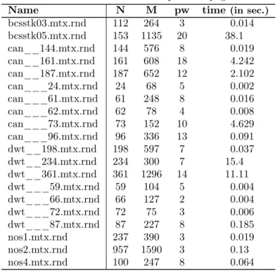
B.3 VSPLIB . . . 33
B.4 Sage . . . 36
1 Average running time of the algorithms on random digraphs. . . 14
2 Computation time for Rome graphs instance . . . 15
3 Average running time of the algorithms on random graphs . . . 27
4 Computation time for instances of the TreewidthLIB with less than 110 nodes . . 28
5 Computation time for instances from the VSPLIB . . . 37
6 Computation time for named graphs inSage . . . 37
7 Computation time for families of graphs inSage . . . 39
List of Tables
1 Versions of the B&B algorithms. . . 122 Repartition of (un)solved instances . . . 15
3 Pathwidth of some Mycielski graphs. . . 16
4 Running time of BAB-GPP for the Mycielski graph M6. . . 16
5 Computational results for twl. instance. . . 28
6 Upper bounds for twl. instance (10 min. per graph). . . 31
7 Computational results for twl-tsp instance. . . 31
8 Upper bounds for twl-tsp instance (10 min. per graph). . . 32
9 Computational results for vsplib_hb instance. . . 33
10 Upper bounds for vsplib_hb instance (10 min. per graph). . . 34
11 Computational results for vsplib_tree instance. . . 35
12 Upper bounds for vsplib_tree instance (10 min. per graph). . . 36
13 Computational results for sage_named instance. . . 38
14 Upper bounds for sage_named instance (10 min. per graph). . . 39
15 Computational results for sage_families instance. . . 40
16 Upper bounds for sage_families instance (10 min. per graph). . . 49
17 Computational results for rome instance. . . 50
Because of their well known algorithmic interest [15], a lot of work has been devoted to the computation oftreewidth and tree-decompositions of graphs [3,33]. On the theoretical side, exact exponential algorithms [6, 20], Fixed Parameter Tractable (FPT) algorithms [8] and Approxi-mation algorithms [5, 19, 31, 36] have been designed. Unfortunately, most of these algorithms can hardly be used in practice. For instance, the algorithm in [6] is both exponential in time and space and therefore cannot be used for graphs with more than 32 nodes. Another example is the FPT algorithms whose time-complexity is at least exponential in the treewidth: there exists no efficient implementation of the Bodlaender and Kloks algorithm [8] even for graphs with treewidth at most 4. On the positive side, efficient algorithms exist for computing the treewidth of particular graph classes, e.g., graphs with treewidth at most 4 [22]. Many heuristics for computing lower or upper bounds on the treewidth have also been designed [1, 9–11].
Surprisingly, much less work has been devoted to the computation of pathwidth and path-decompositions of graphs [3, 32]. Indeed, the pathwidth of any n-node graph is at most O(log n) times its treewidth [3]. Hence, providing an efficient algorithm to compute pathwidth immedi-ately leads to an efficient approximation algorithm for computing the treewidth.
In this paper, we design an algorithm that computes the pathwidth and a corresponding path-decomposition of graphs. We then provide an experimental analysis of our algorithm that presents a significative improvement with respect to existing algorithms.
1.1
Practical computation of pathwidth
Anypath-decomposition of a n-node graph G = (V, E) corresponds to a layout (i.e., an ordering) (v1, · · · , vn) of its vertices. The width of a path-decomposition is the maximum size of the border1
of the subgraphs induced by{v1, · · · , vi}, i ≤ n. The pathwidth of a graph is equal to the
mini-mum width of its path-decompositions. A motivation for computing path-decompositions comes from algorithmic applications. Indeed, given a path-decomposition of a graph, dynamic program-ming algorithms (whose time-complexity depends on the width of the path-decomposition) can be designed for many combinatorial optimization problems [15]. Other motivations arise from the close relationship between pathwidth and other graph invariants (related to node layouts), e.g., the node search number [12,16,30], the process number [14] and the edge search number [25]. Computing the pathwidth of graphs is NP-hard [24] in general and in planar cubic graphs [28] and chordal graphs [21]. An FPT algorithm has been proposed in [8] and some kernelization reduction rules are provided in [7]. However, no polynomial-size kernel is expected [4]. On the practical side, to the best of our knowledge, very few implementations of algorithms for computing the pathwidth (exact or bounds) have been proposed.
Exact algorithms. Solano and Pioro proposed in [37] an exact branch and bound algorithm to compute the pathwidth of graphs, that checks all possible layout of the nodes and keep the best one. A mixed integer linear programming formulation (MILP) has been proposed in [2,37] and a dynamic programming algorithm (exponential both in time and space) is described in [6]. None of these methods handle graphs with more than 30 nodes. As far as we know, the best practical exact algorithm for computing the pathwidth of graphs with more than 30 nodes is based on a SAT formulation of the problem that is solved using Constraint Programming solver [2]. Heuristics. A polynomial-time heuristic for vertex-separation is proposed in [13]. It aims at computing a layout of the nodes in a greedy way . At each step, the next node of the layout is chosen using aflow circulation method. A heuristic based on a branch and bound algorithm has been designed in [37]. Recently, a heuristic has been proposed that is based on the combination
1
switching the nodes until a local optimum is achieved.
1.2
Contributions and organization of the paper
We design a Branch and Bound algorithm that computes the exact pathwidth of graphs and a corresponding path-decomposition. Basically, our algorithm explores the set of all possible layouts of the vertex-set, returning a layout with smallest width. Our main contribution consists of several non-trivial techniques to reduce the size of the input graph (pre-processing) and to cut the exploration space during the search phase of the algorithm. Note that, our algorithm is not restricted to undirected graphs since it actually computes thevertex-separation of digraphs (which coincides with the pathwidth in case of undirected graphs). In Section 2, we prove several technical lemmas that allow us to prove the correctness of the pre-processing phase (Section 2.2) and of the cut procedures (Section 2.3). Section 3 is then devoted to the presentation and the proof of our algorithm. Finally, in Section 4, we evaluate experimentally our algorithm by comparing it to existing algorithms of the literature. It appears from the simulations that our algorithm offers a significative gain with respect to previous work. In particular, it is able to compute the exact pathwidth of any graph with less than 60 nodes in a reasonable running-time (≤ 10 min.). Moreover, our algorithm also achieves good performance when used as a heuristic (i.e., when returning best result found within bounded time-limit).
2
Preliminaries
In this section, we formally define the notions of pathwidth and vertex-separation. Then, we give some technical lemmas which will be used to prove the correctness of our algorithm in next section.
2.1
Definitions and Notations
All graphs and digraphs considered in this paper are connected and loopless. Let G = (V, E) be a graph. For any set S ⊆ V , let NG(S) be the set of nodes in V \ S that have a neighbor
in S. Similarly, for any digraph D = (V, A) and any subset S ⊆ V , let ND+(S) (resp., ND−(S))
be the set of nodes in V \ S that have an in-neighbor (resp., an out-neighbor) in S. We omit the subscript when there is no ambiguity. In the following, we abuse the notations by writing N+(u1, . . . , un) (resp., N−(u1, . . . , un)) instead of N+({u1, . . . , un}) (resp., N−({u1, . . . , un})).
For any digraph D = (V, A) and a = uv ∈ A, let D/a be the graph obtained from D by contracting a. That is, D/a is obtained from D by removing u and v, and adding a new node xuv with ND/a+ (xuv) = ND+(u) ∪ N
+ D(v) \ {u, v} and N − D/a(xuv) = N − D(u) ∪ N − D(v) \ {u, v}. Let
D \ u be the graph obtained from D by removing u and its incident arcs.
Pathwidth. A path-decomposition of a connected graph G = (V, E) is any sequence X = (X1, · · · , Xℓ) of subsets of V such that (1) for any edge {u, v} ∈ E, there exists i ≤ ℓ such
that u, v ∈ Xi, and (2) Xi∩ Xj ⊆ Xk for any 1 ≤ i ≤ k ≤ j ≤ ℓ. The width of X is equal to
maxi≤ℓ|Xi|−1 and the pathwidth of G, pw(G), is the minimum width of the path-decompositions
of G.
Layouts and vertex-separation. Given a set S, a layout of S is any ordering of the elements of S. Let L(S) denote the set of all layouts of S. Let S′⊆ S and P and Q be two layouts of S′
layouts of S with prefix P .
Let D = (V, A) be a digraph and let L = (v1, · · · , v|S|) ∈ L(S) be a layout of S ⊆ V . For
any 1 ≤ i ≤ |S|, let ν(L, i) = |ND+({v1, · · · , vi})| and ν(L) = maxi≤|S|ν(L, i). The
vertex-separation of D, denoted by vs(D), is equal to the minimum ν(L) among all layouts L of V , i.e., vs(D) = minL∈L(V )ν(L).
A digraph D = (V, A) is symmetric if for each arc uv ∈ A, there is vu ∈ A. For any undirected graph G, let vs(G) denote the vertex-separation of the corresponding symmetric digraph obtained from G by replacing each edge {u, v} by two arcs uv and vu. The following result is well known Theorem 1 [23] For any graph G, pw(G) = vs(G).
Therefore, from now on, we will only deal with vertex-separation of digraphs.
2.2
Technical lemmas for preprocessing
In this section, we prove few technical lemmas that will be useful to prove the correctness of the preprocessing part of our algorithm. The following lemmas are known as folklore or have already been proved for undirected graph (i.e., for symmetric digraphs). Due to lack of space, the proofs are omitted and can be found in the Appendix.
Next lemma shows that we can restrict our study to strongly connected digraphs.
Lemma 1 [Folklore] Let D be any connected digraph and let SCC(D) be the set of strongly connected components of D. Then, vs(D) = maxD′∈SCC(D)vs(D′).
In what follows, we show that we can contract some well chosen arcs of a digraph without modifying its vertex-separation. It is well known that, in undirected graphs, edge-contraction cannot increase the pathwidth. However, this is not true anymore in digraphs as shown in the following example. Let D = ({a, b, c, d}, {ab, cb, cd, da}). D is acyclic and therefore, vs(D) = 0. On the other hand, D/cb is a directed cycle with 3 nodes and vs(D/cb) = 1.
Lemmas 2 and 3 explicit conditions under which arc-contractions can be done without in-creasing the vertex-separation.
Lemma 2 Let D = (V, A) be a n-node digraph and uv ∈ A such that either vu ∈ A or N−(v) =
{u}. Then, vs(D) ≥ vs(D/uv).
Lemma 3 Let D = (V, A) be a n-node digraph and u ∈ V such that N+(u) = {v}. Then,
vs(D) ≥ vs(D/uv).
Next lemma show that under some conditions, the vertex-separation does not decrease after arc-contraction.
Lemma 4 Let D = (V, A) be a n-node digraph and uv ∈ A such that,
• vu /∈ A (no loops are created during the contraction) • and
– either N−(v) = {u} and N+(u) ∩ N+(v) = ∅, (v has in-degree 1 and no parallel arcs
out-going from xuv are created during the contraction)
– or N+(u) = {v} and N−(u) ∩ N−(v) = ∅ (u has out-degree 1 and no parallel arcs
From previous lemmas, we get:
Corollary 1 Let D = (V, A) be a n-node digraph and uv ∈ A such that, vu /∈ A, and either (N−(v) = {u} and N+(u) ∩ N+(v) = ∅) or (N+(u) = {v} and N−(u) ∩ N−(v) = ∅). Then,
vs(D) = vs(D/uv). Moreover, an optimal layout for D can be obtained in linear time from an optimal layout of D/uv.
The next lemma is well known in the case of undirected graphs. We extend it to general digraphs.
Lemma 5 Let D = (V, A) be a n-node digraph and let a, b, c ∈ V be three nodes with ND+(b) = ND−(b) = {a, c}, ND+(a) = ND−(a) = {b, x}, ND+(c) = ND−(c) = {b, y}, and x 6= c. Then, vs(D) = vs(D/bc).
2.3
Technical lemmas for the Cut part
In this section, we prove few technical lemmas that will be useful to prove the correctness of the Cut part of our Branch & Bound algorithm.
When looking for a good layout of the nodes of a digraph, our algorithm will, at some step, consider a layout P of some subset S ⊂ V and look for the best layout L of V starting with P . Next lemma gives some conditions on a node v ∈ V \ S to ensure that the best solution starting with P ⊙ v is as good as L.
Lemma 6 Let D = (V, A) be a n-node digraph, S ⊂ V , and P ∈ L(S). If there exists v ∈ V \ S such that either N+(v) ⊆ (S ∪ N+(S)), or v ∈ N+(S) and N+(v) \ (S ∪ N+(S)) = {w}. Then,
minL∈LP(V )ν(L) = minL∈LP⊙{v}(V )ν(L).
Assume we know the best layout L of V having a prefix P . The next lemma expresses some conditions under which no layout of V starting with a permutation of P is better than L. Lemma 7 Let D = (V, A) be a n-node digraph, S ⊂ V and let P, P′ ∈ L(S) be two layouts of
S. If ν(P ) < minL∈LP(V )ν(L) or ν(P ) ≤ ν(P
′), then min
L∈LP(V )ν(L) ≤ minL∈LP ′(V )ν(L).
3
The algorithm
In this section, we present our exact exponential-time algorithm for computing vs(D) for any n-node digraph D = (V, A). To ease the presentation, we assume that D is strongly connected. If it is not the case, we apply all the steps of our algorithm to each of its strongly connected components, and then use the construction presented in the proof of Lemma 1 to deduce in linear time the layout L of D such that ν(L) = vs(D).
Our algorithm is based on a Branch & Bound procedure that considers all possible layouts of V and keeps a layout L minimizing ν(L). Since the worst case time-complexity of such an algorithm is O(n!), we first do a pre-processing to reduce the size of the input.
Require: A digraph D = (V, A), a layout P of S ⊆ V 1: S := V (P ) and P′ := P 2: while ∃ v ∈ V \ S s.t. N+(v) ⊆ S ∪ N+(S) or ∃ v ∈ N+(S) s.t. |N+(v) \ (S ∪ N+(S))| = 1 do 3: P′:= P ⊙ v and S := S ∪ {v} 4: return P′
Algorithm 2 Update-prefix-table(D, P, P, Current, vs∗).
1: if vs∗< Current and ν(P ) = vs∗ then b := 0 else b := 1 2: if (V (P ), ν(P ), 0) ∈ P then
3: Replace (V (P ), ν(P ), 0) with (V (P ), ν(P ), b) in P 4: else
5: Add (V (P ), ν(P ), b) in P
3.1
Pre-processing phase
The following reduction rules are applied while it is possible. The rules that have been proposed for undirected graphs can be used only when D is a symmetric digraph. Note that, the digraph D∗ obtained after applying once one of these rules is strongly connected, and that given the
layout L∗ such that ν(L∗) = vs(D∗), one can deduce in linear time a layout L for D such that
ν(L) = vs(D).
Rule A: If there is uv ∈ A such that, vu /∈ A, and either (N−(v) = {u} and N+(u) ∩ N+(v) =
∅), or (N+(u) = {v} and N−(u) ∩ N−(v) = ∅), then let D∗ = D/uv (By Corollary 1,
vs(D∗) = vs(D)).
Rule B: If there are three nodes a, b, c ∈ V with ND+(b) = ND−(b) = {a, c}, ND+(a) = ND−(a) = {b, x}, ND+(c) = ND−(c) = {b, y}, and x 6= c, then let D∗= D/bc (By Lemma 5, vs(D∗) =
vs(D)).
Rule C: If D is symmetric, let G be the underlying undirected graph. It is shown in [7] that vs(D∗) = vs(D) when D∗ is obtained as follows.
C.1: If (in G) two degree-one vertices u and v share their neighbor, then D∗= D \ u.
C.2: If (in G) v, w are two vertices of degree two, and suppose x and y are the common neighbors of v and w, then D∗= D/vx.
Note that, each time that one of the above rules is applied, the number of nodes decreases by one and therefore, the worst case time-complexity is divided by n.
When no reduction rules can be applied anymore, the algorithm B&B is applied as explained below.
3.2
Branch & Bound phase
We now describe our Branch & Bound, that we call B&B. The main contribution of our work consists of the way we cut the exploration of all layouts of V . Intuitively, let S ⊂ V and P be a layout of S that Procedure B&B is testing, i.e., let us consider a step when B&B is considering all layouts of V with prefix P . Moreover, let LU B be the best layout of D obtained so far by
1: if ν(P ) < vs∗ and (V (P ), ν(P ), 1) /∈ P then 2: P′:= Greedy(D, P ) 3: if V (P′) = V and ν(P′) < vs∗ then 4: return (ν(P′), P′) 5: else 6: Current := vs∗
7: for all v ∈ V \ P′, by increasing values of ν(P′⊙ v) do
8: if ν(P′⊙ v) < vs∗ then 9: (vs′′, L′′) := B&B(D, P′⊙ v, vs∗, L∗, P) 10: if vs′′< vs∗ then 11: (vs∗, L∗) := (vs′′, L′′) 12: Update-prefix-table(D, P, P, Current, vs∗) 13: return (vs∗, L∗)
1. Decide, based on Lemma 7, if it is useful to explore layouts with prefix P . For this purpose, we maintain a tableP that contains, among other, some subsets of V . If there is an entry inP for S ⊂ V and satisfying some properties, we can decide that the best layout starting with the nodes in S cannot be better than LU B and therefore, we do not test further layouts
with prefix P .
2. Greedily extend the current prefix P with a vertex v ∈ V \ S, with S = V (P ), if v satisfies the conditions of Lemma 6. This allows us to restrict the exploration of all the layouts with prefix P to the layouts with prefix P ⊙ v.
As shown in the next section, these two cutting rules allow our algorithm to achieve better performances than existing algorithms for computing the vertex-separation of digraphs.
Let us now describe the Procedure B&B (Algorithm 3) more formally and prove its correct-ness. This recursive procedure takes as inputs:
• D = (V, A), the considered digraph.
• LU B and U B such that LU B is the best layout of V obtained so far and U B = ν(LU B).
Note that U B is an upper bound for (vs(D).
• P , a layout of a subset S ⊆ V . Intuitively, P is the prefix of the layouts that will be tested by this execution of B&B. That is, either Procedure B&B will find a layout L = P ⊙ Q of V such that ν(L) < ν(LU B) or it decides that ν(L) ≥ ν(LU B) for any L ∈ LP(V ).
• P is a set of triples (Si, νi, bi)i≤ρ, where Si⊂ V , νiis an integer, and biis a boolean for any
i ≤ ρ. Intuitively, (Si, νi, bi) ∈ P means that a layout Pi of Si has already been checked,
and, if bi= 1, then it is useless to test any other layout of V starting with the nodes in Si.
Moreover, νi = ν(Pi) and bi= 0 if νi= minL∈LPi(V )ν(L).
The initial values for the inputs of B&B are: P = ∅, LU B is any layout L of V and U B = ν(L) <
|V |, and P = ∅.
Let P = (Si, νi, bi)i≤ρ and (LU B, U B) be the current values of the global variables at some
step of the execution of the algorithm. Then, executing B&B(D, P, U B, LU B, P), with P =
layouts starting by P stops. Indeed, by definition, minL∈LP(V )ν(L) ≥ ν(P ). Therefore,
minL∈LP(V )ν(L) ≥ U B and no layout of V starting with P can be better than LU B.
• else, if (S, x, b) belongs to P then this means that a layout P′ of S has been already
tested, x = ν(P′) and U B ≤ min
L∈LP ′(V )ν(L). If b = 1 or ν(P ) ≥ ν(P
′), then
B&B(D, P, U B, LU B, P) does nothing, i.e., the exploration of the layouts starting by P
stops. Indeed, either x < minL∈LP ′(V )ν(L) (if b = 1) or ν(P ) ≥ ν(P
′). By Lemma 7, it
implies that minL∈LP ′(V )ν(L) ≤ minL∈LP(V )ν(L). Again, no layout of V starting with P
can be better than LU B.
• otherwise, B&B(D, P, U B, LU B, P) applies the sub-procedure Greedy(D, P ) (Algorithm 1)
that returns a prefix P′ extending P (i.e., P is a prefix of P′) and min
L∈LP(V )ν(L) =
minL∈LP ′(V )ν(L). Then, it calls B&B(D, P
′⊙ v, U B, L
U B, P) for all v ∈ V \ V (P′) such
that ν(P′⊙ v) < U B, starting from the most promising vertices (i.e., by increasing value
of ν(P′⊙ v)).
At the end of the exploration of the layouts with prefix P , we update the table P (Algo-rithm 2). That is,
– if there was no triple (S, ∗, ∗) in P, then, (S, ν(P ), b) is added to P with b = 0 if and only if ν(P ) = ν(L∗).
– else, i.e., if there is (S, x, 0) ∈ P with ν(P ) < x and ν(P ) < U B, then, (S, ν(P ), b) replaces (S, x, 0) in P with b = 0 if and only if ν(P ) = ν(L∗).
4
Simulations and interpretation of results
In this section, we evaluate the performance of our algorithm. In particular, we compare it to other exact algorithms and heuristics from the literature. We also analyze the impact of the three optimization phases of our algorithm : pre-processing, greedy steps, and cuts using prefixes. It appears that our algorithm is able to compute the vertex-separation of all graphs with at most 60 nodes but also for some graphs up to 250 nodes. Not only our algorithm outperforms the performance of existing exact algorithms but it can also be used as a good heuristic to obtain upper bounds on the vertex-separation.
4.1
Implementation
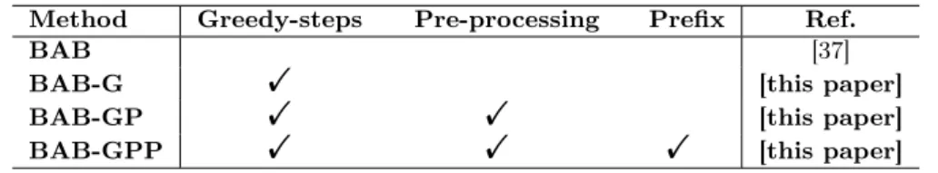
We have implemented several variants of our Branch and Bound algorithm in order to analyze the impact of each of our optimization sub-procedures. Our algorithms are implemented in Cython using the Sage open-source mathematical software [38]. All computations have been performed on a computer equipped with a Intel Xeon CPU operating at 3.20GHz and 64GB of RAM. Note that, all the algorithms take a digraph as an input. If the input is a non-directed graph, we consider it as a symmetric directed graph. We now present our variants of the Branch and Bound algorithm (Tab. 1).
BAB. This is the basic version of the branch and bound algorithm (as already implemented in [37]). It takes digraph as an input D and is applied sequentially on each of the strongly connected components of D. For each strongly connected component C of D, BAB con-siders all possible layouts of V (C) and keeps a layout L minimizing ν(L).
BAB [37]
BAB-G ✦ [this paper]
BAB-GP ✦ ✦ [this paper] BAB-GPP ✦ ✦ ✦ [this paper]
Table 1: Versions of the B&B algorithms.
BAB-G. In this variant, we add the greedy-step process (Algorithm 1) to the basic variant BAB.
BAB-GP. In this variant, we add the pre-processing phase to the variant BAB-G. That is, if some arc-contractions or node-deletions can be performed on the input digraph, we execute them.
BAB-GPP. This last variant is our main algorithm which is obtained from BAB-GP by adding a cut-process by storing some subsets of nodes a layout of which has already been tested as prefix (Algorithm 2).
For the different variants, it is critical to have a fast access to the data structure representing the digraph. To speed-up critical operations on neighborhoods (union, intersection, size, etc.), we store out-neighborhoods using bitsets (in particular, a single integer when n ≤ 64). This enables us to use bitwise operations (or for union, and for intersection, etc.).
For BAB-GPP, the prefixes are stored in a tree structure which allows us a fast access to already tested prefixes. We parameterized the maximum length of a prefix (which corresponds to the tree depth) and set it by default to min{n/3, 50}. The total number of stored prefixes is also parameterized to limit memory usage. By default we store at most 106 prefixes.
Finally, we used a timer to limit computation time per (di)graph. When the time is up, we return the best solution found so far and record it as an upper-bound on the vertex-separation of the input digraph. Following [2], we set this limit to 10 min.
Previous exact algorithms. The pathwidth problem is known to be Fixed Parameter Tractable, that is, vs(G) ≤ k can be decided in time f (k)|V (G)| [8]. However, the function f is of order O(2kc
) for some c ≥ 2. Moreover, there is few hope to obtain a better function since pathwidth is unlikely to have a polynomial kernel [4]. Therefore, such algorithms have not been implemented and people have focused on exact exponential-time algorithms.
In addition to the basic Branch and Bound BAB of Solano [37], we are aware of the following implementations of algorithms to compute vertex-separation of graphs.
MILP. Some mixed integer linear programming formulations for the vertex-separation (MILP) have been proposed in [2, 37]. A similar formulation has been implemented in Sage2
. We use this function for purpose of comparison.
DYNPROG. In [6], a dynamic programming algorithm, called DYNPROG, is designed to compute the vertex-separation of a digraph D. Roughly, this algorithm aims at deciding whether vs(D) ≤ k for all k = 1, · · · , |V (D)|. For a given k ≤ |V (D)|, DYNPROG stores the subsets of V (D) with border at most k and uses dynamic programming to limit the number of stored subsets. An implementation of DYNPROG is also available in Sage2
. 2
for graphs with strictly less than 32 nodes.
SAT. In [2], an algorithm to compute the pathwidth of graphs is designed by formulating the PATHWIDTH problem as a Boolean satisfiability testing (SAT) instance and solving this SAT instance using the M iniSat solver [26]. No implementations are provided but the algorithm has been tested on theRome graphs dataset [34]. The SAT algorithm have been able to compute the pathwidth of 17% of the instances in the Rome graphs dataset.
4.2
Comparison of our algorithms with BAB, MILP, and DYNPROG
in random digraphs
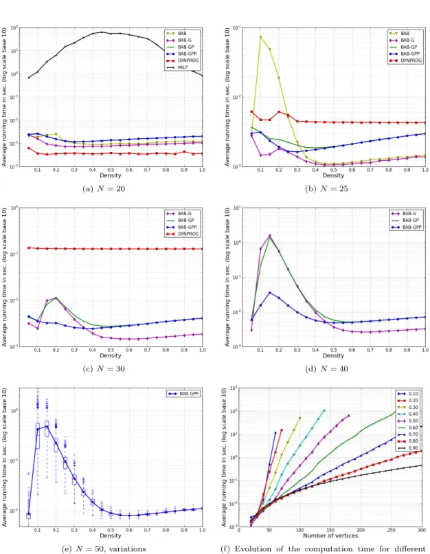
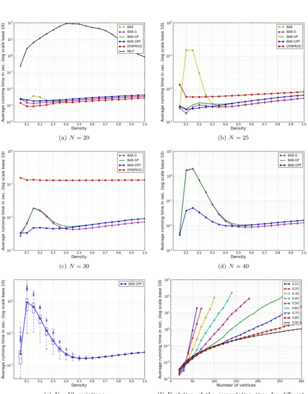
In this section, we use the available implementations of MILP and DYNPROG inSage to compare their performance with our algorithms in random directed graphs. Random directed graphs with N nodes are generated using the graphs.RandomDirectedGNM(N,M) method of Sage to generate them, where M = density ∗ N (N − 1) is the number of arcs. For several network sizes (N ∈ {20, 25, 30, 40, 50}), we execute the algorithms for various densities (0 < density < 1). For each size N and each density, we run the algorithms on 1 000 instances. The same instances are used for all algorithms. The average running times are depicted on Fig. 1.
Small graphs (N = 20). Fig. 1(a) shows that the MILP Algorithm is out-performed by all other algorithms even for N = 20. In particular, two weeks of computations have been required to generate Fig. 1(a) because of MILP. Fig. 1(a) also shows that, for N = 20, Algorithm DYNPROG is slightly faster than all variants of BAB. In particular, the running time of BAB-GPP is a bit larger than for other variants. This is probably due to the fact that the cuts on the exploration space done by the optimization procedures executed by BAB-GPP are negligible compared with the time needed to apply the optimization procedures.
Graphs with N ∈ {25, 30}. Figs. 1(b) and 1(c) show that, for graphs with at least 25 nodes, our algorithms become competitive with respect to DYNPROG. In particular, for graphs with 30 nodes, our algorithms are significantly faster (Recall that DYNPROG can only used for graphs with at most 31 nodes).
Impact of optimization Phases. In Figs. 1(b) to 1(e), we observe that for densities ≥ 0.4, all variants of the branch and bound algorithm are very fast with negligeable differences (≤ 0.01 sec.). However, we observe large variations for smaller densities. More precisely, we observe in Fig. 1(b) the significant speed-up offered by the Greedy steps w.r.t. the basic branch and bound proposed in [37]. The benefits of the pre-processing phases are however difficult to observe on such small random digraphs since the conditions required to contract arcs rarely occur, and so we observe an improvement in Fig. 1(d) only when the density is 0.05. However, Fig. 1(d) reports large speed-up when using prefixes to cut the search space. In Fig. 1(e), we point out that the running time of BAB-GPP varies a lot depending on the graphs (especially for graphs with small density). We report on the variations in running time when N = 50 and using the best settings of our algorithm. For densities below 0.4 the running time varies by up to two orders of magnitude, while for larger densities, the range of variations is very small. Last, we have reported in Fig. 1(f) the evolution of the running time of BAB-GPP for different densities. This confirms that the higher the density, the larger the size of the graphs we are able to solve. Note that we have observed the same behaviors for all algorithms with symetric digraphs (and so undirected graphs).
4.3
Comparison of BAB-GPP with SAT on the Rome graphs dataset
(a) N = 20 (b) N = 25
(c) N = 30 (d) N = 40
(e) N = 50, variations (f) Evolution of the computation time for different densities. Average values over 100 digraphs.
Solved 9586 85 77 68 65 62 65 59 50 96 91 104 113 91 110 80 77 70 78 11 027
Unsolved 0 1 1 5 5 6 4 4 9 20 28 30 41 48 38 59 66 74 63 502
Table 2: Repartition of (un)solved instances for the Rome graph Instance.
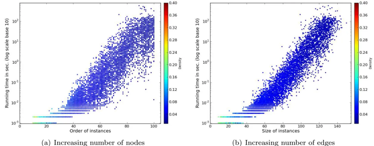
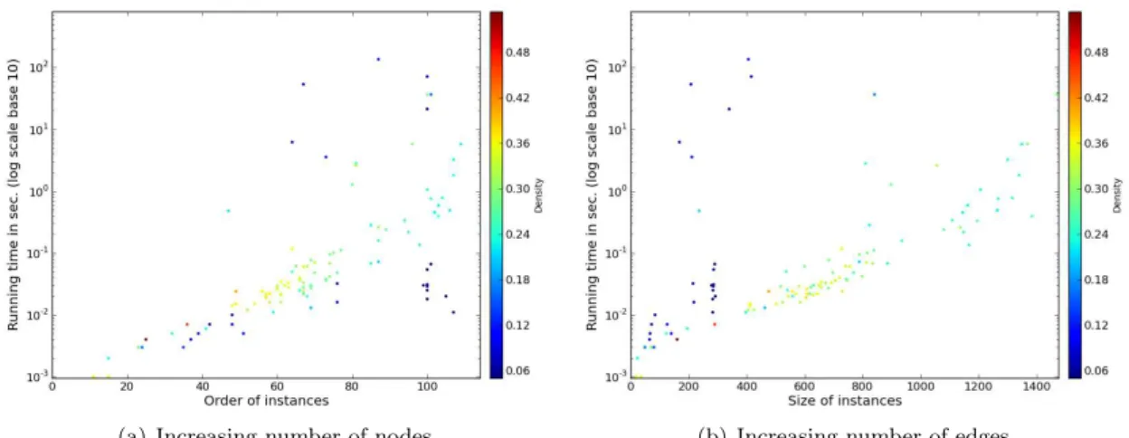
(a) Increasing number of nodes (b) Increasing number of edges
Figure 2: Computation time for Rome graphs. One dot per instance. The color indicates the density of the instance.
In [2], the performance of the SAT algorithm has been evaluated using this benchmark. With 10 min. time limit per graph, the algorithm of [2] has been able to compute the pathwidth for 17.0% of the Rome graphs. In particular, it is stated that “We note that almost all small graphs (n+m < 45) could be solved within the given timeout, however, for larger graphs, the percentage of solved instances rapidly drops [. . . ] Almost no graphs with n+m > 70 were solved." [2] (where m is the number of edges of the considered graphs).
In contrast, our algorithm has computed the pathwidth of 95.6% of the graphs in theRome dataset, with same time limit of 10 min. Note that, in particular, we solved all instances with at most 82 vertices. We report in Tab. 2 the repartition of (un)solved instances and in Fig. 2 the computation time per solved graphs.
4.4
Impact of prefix length
Our main algorithm BAB-GPP is parameterized by the maximum length of the prefixes that we store and that allow us to cut the search space during the branch and bound process. We have evaluated the impact of this parameter when our algorithm is executed on some specific graphs. In particular, the Mycielski graph is considered as a hard instance for integer programming formulations for pathwidth [27]. The Mycielski graph Mkis a triangle-free graph with chromatic
number k having the smallest possible number of vertices. See [29] for a formal definition of Mk.
Note that,|V (M2)| = 2 and |V (Mk)| = 2|V (Mk−1)| + 1 for any k > 2. We ran our algorithm on
the Mycielski graph Mk for k ≤ 8. The results we obtained are depicted in Tab. 3 (for k ∈ {7, 8}
we only got upper bounds).
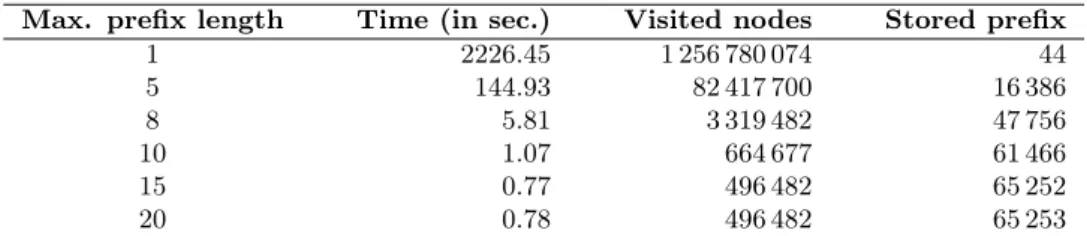
Tab. 4 presents the running time of BAB-GPP for the Mycielski graph M6 and different
|V (Mk)| 1 2 5 11 23 47 95 191
pw(Mk) 0 1 2 5 10 20 ≤ 38 ≤ 72 Table 3: Pathwidth of some Mycielski graphs.
Max. prefix length Time (in sec.) Visited nodes Stored prefix 1 2226.45 1 256 780 074 44 5 144.93 82 417 700 16 386 8 5.81 3 319 482 47 756 10 1.07 664 677 61 466 15 0.77 496 482 65 252 20 0.78 496 482 65 253
Table 4: Running time of BAB-GPP for the Mycielski graph M6.
number of nodes of the branch and bound exploration space that are actually considered. Tab. 4 shows that storing larger prefixes allows for an impressive reduction of the computation time. However, we have no improvement here when allowing length of 20 instead of 15, and larger values behave similarly. This is probably due to the fact that in this experiment, because of the greedy steps, the algorithm stores only one prefix of length≥ 15.
This suggests that the combination of the greedy steps and of the storage of the prefixes allows good performances even when the length of the prefixes is bounded. Therefore, memory-space seems not to be an issue for graphs of reasonable size (while the algorithm might potentially store an exponential number of prefixes).
4.5
Using BAB-GPP as an heuristic
Since computing the optimal vertex-separation of a graph is NP-hard, some research has been devoted to design heuristic algorithms for this problem. In [17], an local-search based heuristic is designed: starting from some layout of the nodes of D, the solution is improved by locally switching consecutive nodes in the layout until no further improvement can be obtained. The VSPLIB [40] has been designed for benchmarking this heuristic [17]. VSPLIB [40] contains 173 instances: 50 n × n grids with 5 ≤ n ≤ 54; 50 trees with respectively 22, 67, and 202 nodes and pathwidth 3, 4, and 5; a set of 73 graphs, called hb, with n ≤ 10 ≤ 960 (see [17] for more details). In particular, the pathwidth of n × n grids equals n and the pathwidth of trees can be computed in linear time [18, 35]. Therefore, this benchmark allows to evaluate the performance of heuristic.
We used Algorithm BAB-GPP as an heuristic: if the time is up before the end of its execution, the algorithm returns the value computed so far (i.e., an upper bound on the vertex-separation of the graph).
We were able to compute the exact pathwidth for the grids with side n ≤ 13, the trees with n ≤ 67, and 26 of the hb graphs including one with 957 nodes. More interestingly, for all grids and trees of the VSPLIB, the final value returned by BAB-GPP equals the exact pathwidth. That is, our algorithm always finds quickly an optimal layout and most of the execution time is devoted to prove its optimality.
In particular for a n × n grid, the first solution found is always the pathwidth. This is due to the order in which we add the vertices in the layouts: starting from a node with smallest degree and always adding a node that minimizes the increase of the size of the border. Proceeding that
For trees, the first layout tested by BAB-GPP is not always the optimal one, but an optimal one is found very quickly. It would be interesting to understand why our branch and bound algorithm performs well in trees.
5
Conclusion
In this paper, we have presented a new branch and bound algorithm for computing the pathwidth of graphs and the vertex-separation of digraphs. This algorithms combines new pre-processing rules for reducing the size of the input digraph and new cutting rules allowing for significantly reducing the search space. Experimental validation of our algorithm on benchmark instances suggest that our approach is more promizing than previous proposals, based on ILP or SAT, for solving large instances. Indeed, the drawbacks of ILP and SAT formulations for layout problems are both in the large number of symmetries of the problems, and in the time needed to fill the optimality gap (i.e., distance between the lower bound based on the fractional relaxation of the formulation and the best integral solution).
Our next steps are on one hand to propose our code for inclusion into future releases ofSage. On the other hand, we will search for new cutting rules to further reduce computation time. In particular, looking for good lower bounds for pathwidth of graphs is a theoretical issue that received few attention. It would moreover speed up our algorithm since the main computation time seems dedicated to prove the optimality of the best value computed.
References
[1] E. H. Bachoore and H. L. Bodlaender. New upper bound heuristics for treewidth. In 4th InternationalWorkshop on Experimental and Efficient Algorithms (WEA), volume 3503 of Lecture Notes in Computer Science, pages 216–227. Springer, 2005.
[2] T. C. Biedl, T. Bläsius, B. Niedermann, M. Nöllenburg, R. Prutkin, and I. Rutter. Using ILP/SAT to determine pathwidth, visibility representations, and other grid-based graph drawings. In Graph Drawing, volume 8242 of Lecture Notes in Computer Science, pages 460–471. Springer, Sept. 2013.
[3] H. L. Bodlaender. A partialk-arboretum of graphs with bounded treewidth. Theor. Comput. Sci., 209(1-2):1–45, 1998.
[4] H. L. Bodlaender, R. G. Downey, M. R. Fellows, and D. Hermelin. On problems without polynomial kernels. J. Comput. Syst. Sci., 75(8):423–434, 2009.
[5] H. L. Bodlaender, P. G. Drange, M. S. Dregi, F. V. Fomin, D. Lokshtanov, and M. Pilipczuk. An o(ckn) 5-approximation algorithm for treewidth. In 54th Annual IEEE Symposium on
Foundations of Computer Science (FOCS), pages 499–508. IEEE Computer Society, 2013. [6] H. L. Bodlaender, F. V. Fomin, A. M. Koster, D. Kratsch, and D. M. Thilikos. A note on
exact algorithms for vertex ordering problems on graphs. Theory Comput. Syst., 50(3):420– 432, 2012.
[7] H. L. Bodlaender, B. M. P. Jansen, and S. Kratsch. Kernel bounds for structural parameteri-zations of pathwidth. In13th Scandinavian Symposium and Workshops on Algorithm Theory (SWAT), volume 7357 of Lecture Notes in Computer Science, pages 352–363. Springer, 2012.
treewidth of graphs. J. Algorithms, 21(2):358–402, 1996.
[9] H. L. Bodlaender and A. M. C. A. Koster. On the maximum cardinality search lower bound for treewidth. Discrete Applied Mathematics, 155(11):1348–1372, 2007.
[10] H. L. Bodlaender and A. M. C. A. Koster. Treewidth computations i. upper bounds. Inf. Comput., 208(3):259–275, 2010.
[11] H. L. Bodlaender and A. M. C. A. Koster. Treewidth computations ii. lower bounds. Inf. Comput., 209(7):1103–1119, 2011.
[12] R. L. Breisch. An intuitive approach to speleotopology. Southwestern Cavers, VI(5):72–78, 1967.
[13] D. Coudert, F. Huc, D. Mazauric, N. Nisse, and J.-S. Sereni. Reconfiguration of the routing in WDM networks with two classes of services. InProc. ONDM, pages 1–6, Braunschweig, Germany, Feb. 2009. IEEE.
[14] D. Coudert, S. Perennes, Q.-C. Pham, and J.-S. Sereni. Rerouting requests in WDM net-works. InProc. AlgoTel, pages 17–20, 2005.
[15] B. Courcelle and M. Mosbah. Monadic second-order evaluations on tree-decomposable graphs. Theor. Comput. Sci., 109(1&2):49–82, 1993.
[16] J. Díaz, J. Petit, and M. Serna. A survey on graph layout problems.ACM Comput. Surveys, 34(3):313–356, 2002.
[17] A. Duarte, L. F. Escudero, R. Martí, N. Mladenovic, J. J. Pantrigo, and J. Sánchez-Oro. Variable neighborhood search for the vertex separation problem. Computers & OR, 39(12):3247–3255, 2012.
[18] J. Ellis, I. Sudborough, and J. Turner. The vertex separation and search number of a graph. Inform. Comput., 113(1):50–79, 1994.
[19] U. Feige, M. T. Hajiaghayi, and J. R. Lee. Improved approximation algorithms for minimum-weight vertex separators. In 37th Annual ACM Symposium on Theory of Computing (STOC), pages 563–572. ACM, 2005.
[20] V. Gogate and R. Dechter. A complete anytime algorithm for treewidth. CoRR, abs/1207.4109, 2012.
[21] J. Gustedt. On the pathwidth of chordal graphs. Discrete Applied Mathematics, 45(3):233– 248, 1993.
[22] A. Hein and A. M. C. A. Koster. An experimental evaluation of treewidth at most four reductions. In 10th International Symposium on Experimental Algorithms (SEA), volume 6630 ofLecture Notes in Computer Science, pages 218–229. Springer, 2011.
[23] N. G. Kinnersley. The vertex separation number of a graph equals its pathwidth. Inform. Process. Lett., 42(6):345–350, 1992.
[24] M. Kirousis and C. Papadimitriou. Searching and pebbling. Theo. Comp. Sci., 47(2):205– 218, 1986.
complexity of searching a graph. J. ACM, 35(1):18–44, 1988.
[26] MiniSat, a minimalistic open-source SAT solver. http://minisat.se/. [27] MIPLIB - mixed integer problem library. http://miplib.zib.de/.
[28] B. Monien and I. H. Sudborough. Min cut is np-complete for edge weighted trees. Theor. Comput. Sci., 58:209–229, 1988.
[29] J. Mycielski. Sur le coloriage des graphes. Colloquium Mathematicum, 3:161–162, 1955. [30] T. D. Parsons. Pursuit-evasion in a graph. InTheory and applications of graphs, volume
642 ofLecture Notes in Mathematics, pages 426–441. Springer, Berlin, 1978.
[31] B. A. Reed. Finding approximate separators and computing tree width quickly. In 24th Annual ACM Symposium on Theory of Computing (STOC), pages 221–228. ACM, 1992. [32] N. Robertson and P. D. Seymour. Graph minors. i. excluding a forest. J. Comb. Theory,
Ser. B, 35(1):39–61, 1983.
[33] N. Robertson and P. D. Seymour. Graph minors. III. Planar tree-width. J. Combin. Theory Ser. B, 36(1):49–64, 1984.
[34] Rome graphs. http://www.graphdrawing.org/download/rome-graphml.tgz.
[35] P. Scheffler. A linear algorithm for the pathwidth of trees. In R. H. R. Bodendiek, editor, Topics in Combinatorics and Graph Theory, pages 613–620. Physica-Verlag Heidelberg, 1990.
[36] P. D. Seymour and R. Thomas. Call routing and the ratcatcher. Combinatorica, 14(2):217– 241, 1994.
[37] F. Solano and M. Pióro. Lightpath reconfiguration in WDM networks. IEEE/OSA J. Opt. Commun. Netw., 2(12):1010–1021, Dec. 2010.
[38] W. Stein et al. Sage Mathematics Software (Version 6.0). The Sage Development Team, 2013. http://www.sagemath.org.
[39] J.-W. van den Broek and H. Bodlaender. TreewidthLIB, a benchmark for algorithms for treewidth and related graph problems. http://www.cs.uu.nl/research/projects/ treewidthlib/.
A.1
Proofs of technical lemmas for pre-processing
Lemma 1 (Folklore) Let D be any connected digraph and let SCC(D) be the set of strongly connected components of D. Then, vs(D) = maxD′∈SCC(D)vs(D′).
Proof. Let L be any layout of D and let D′ ∈ SCC(D). Let L′ be the corresponding layout of
D′ (that is, for any u, v ∈ V (D′), u appears before v in L′ if and only if u appears before v in
L). Then, ν(L′) ≤ ν(L).
Conversely, for any D′ ∈ SCC(D), let L
D′ be an optimal layout of D′. For any D′, D′′ ∈
SCC(D), we set D′ ≺ D′′ if there is a path from D′′ to D′. Note that, in this case, there
is no path from D′ to D′′, and therefore ≺ is a partial order. Let L be the layout of D
ob-tained by concatenating the layouts in (LD′)D′∈SCC(D) in such a way that LD′′ is after LD′
if D′ ≺ D′′ for all D′, D′′ ∈ SCC(D) (this is possible since ≺ is a partial order). Then
ν(L) ≤ maxD′∈SCC(D)ν(LD′).
Lemma 2 Let D = (V, A) be a n-node digraph and uv ∈ A such that either vu ∈ A or N−(v) =
{u}. Then, vs(D) ≥ vs(D/uv).
Proof. Let L = (v1, · · · , vn) be a layout of V with {u, v} = {vi, vj} and i < j.
Let us consider the layout L′ = (v′
1, · · · , vn−1′ ) = (v1, · · · , vi−1, vi+1, · · · , vj−1, xuv, vj+1, · · · , vn)
of V (D/uv)3
. Let 1 ≤ k < n − 1, w ∈ ND/uv+ (v1′, · · · , v′k) and let x ∈ {v1′, · · · , v′k} such that
xw ∈ A(D/uv). Let Nk = N+ D(v1, · · · , vk) if k < i, and Nk = N + D(v1, · · · , vk+1) if i ≤ k < j − 1, and Nk= N+ D(v1, · · · , vk+2) if k ≥ j − 1. • If w 6= xuv, then
– either x 6= xuv and xw ∈ A(D) and w ∈ Nk.
– or x = xuv, then k ≥ j − 1, w /∈ {u, v} and either uw ∈ A(D) or vw ∈ A(D).
Therefore, w ∈ Nk.
• If w = xuv then k < j − 1 and either xu ∈ A(D) or xv ∈ A(D).
– if k < i, then either u or v belong to Nk since xu ∈ A(D) or xv ∈ A(D).
– otherwise, i ≤ k < j − 1 and, by hypothesis on u and v: ∗ either vivj∈ A, in which case vj∈ Nk,
∗ or vi = v, vj = u and we have that xu ∈ A(D), since N−(v) = {u} and x 6= u
(i.e., xv /∈ A(D)). Therefore, xu ∈ A(D) and u ∈ Nk.
In all cases, we get that|N+
D/uv(v1′, · · · , vk′)| ≤ |Nk| and therefore, for all layouts L of D there
is a layout L′ of D/uv such that ν(L′) ≤ ν(L). Hence, vs(D/uv) ≤ vs(D).
3
Here, to simplify the presentation, we slightly abuse the notations by identifying the nodes of D \ {u, v} and the nodes of (D/uv) \ {xuv}.
vs(D) ≥ vs(D/uv).
Proof. Let L = (v1, · · · , vn) be a layout of V with {u, v} = {vi, vj} and i < j. The case vivj ∈ A
is similar to the one of previous lemma. Therefore, let us assume that vi = v and vu /∈ A. Let
us consider the layout L′ = (v′
1, · · · , v′n−1) = (v1, · · · , vi−1, xuv, vi+1, · · · , vj−1, vj+1, · · · , vn) of
V (D/uv). Let 1 ≤ k < n − 1, w ∈ ND/uv+ (v′
1, · · · , v′k) and let x ∈ {v1′, · · · , v′k} such that
xw ∈ A(D/uv). Let Nk = N+
D(v1, · · · , vk) if k < i, Nk = ND+(v1, · · · , vi−1, v = vi, · · · , vk) if i ≤ k < j, and
Nk= N+
D(v1, · · · , vi−1, v, vi+1, · · · , vj−1, u, vj+1, · · · , vk+1) if k ≥ j.
• If w, x 6= xuv, then xw ∈ A(D) and w ∈ Nk.
• If w = xuv then k < i, x /∈ {u, v}, and either xu ∈ A(D) or xv ∈ A(D). Hence, u or v
belongs to Nk.
• If x = xuv then k ≥ i, w /∈ {u, v}, either uw ∈ A(D) or vw ∈ A(D). But v being the single
out-neighbor of u and v 6= w, we get that vw ∈ A(D), and therefore, w ∈ Nk.
In all cases, we get that|N+
D/uv(v1′, · · · , v′k)| ≤ |Nk| and therefore, for all layouts L of D there is
a layout L′ of D/uv such that ν(L′) ≤ ν(L). Hence, vs(D/uv) ≤ vs(D).
Lemma 4 Let D = (V, A) be a n-node digraph and uv ∈ A such that,
• vu /∈ A (no loops are created during the contraction) • and
– either N−(v) = {u} and N+(u) ∩ N+(v) = ∅, (v has in-degree 1 and no parallel arcs
out-going from xuv are created during the contraction)
– or N+(u) = {v} and N−(u) ∩ N−(v) = ∅ (u has out-degree 1 and no parallel arcs
in-going to xuv are created during the contraction).
Then, vs(D) ≤ vs(D/uv). Proof. Let L′ = (v
1, · · · , vi−1, xuv, vi+1, · · · , vn−1) be any optimal layout of D/uv.
Case: vkv /∈ A for any k < i, i.e., v /∈ ND+(v1, · · · , vj). Note that, in particular, it is the case
when N−(v) = {u}.
Let L1= (v1, · · · , vi−1, v, u, vi+1, · · · , vn−1) and L2= (v1, · · · , vi−1, v, u, vi+1, · · · , vn−1).
We show that ν(L1) ≤ ν(L′) or ν(L2) ≤ ν(L′).
1. Let j < i and w ∈ ND+(v1, · · · , vj). Since v /∈ ND+(v1, · · · , vj), w 6= v.
• If w 6= u, then w ∈ ND/uv+ (v1, · · · , vj).
• Otherwise, there is vh, h ≤ j such that vhu ∈ A(D) and so vhxuv ∈ A(D/uv)
and, thus, xuv∈ ND/uv+ (v1, · · · , vj).
Hence, in both cases,|N+
D(v1, · · · , vj)| ≤ |N +
D/uv(v1, · · · , vj)|.
2. Let j > i and w ∈ ND+(v1, · · · , vj). Since w /∈ {u, v}, then
uv D 1 i−1 D 1 i−1 D/uv 1 i−1 uv
4. It remains to show that|ND+(v1, · · · , vi−1, v)| ≤ ν(L′) or |ND+(v1, · · · , vi−1, u)| ≤ ν(L′)
First, note that ND+(v1, · · · , vi−1, v) = (ND+(v1, · · · , vi−1)\{v})∪(ND+(v)∩{u, vi+1, · · · , vn−1}).
Moreover, since v /∈ ND+(v1, · · · , vi−1) and vu /∈ A, this implies that
ND+(v1, · · · , vi−1, v) = ND+(v1, · · · , vi−1) ∪ (ND+(v) ∩ {vi+1, · · · , vn−1}). (1)
On the other hand, by definition, we have that ND+(v1, · · · , vi−1, v, u) = (ND+(v1, · · · , vi−1)\{u})
[
((ND+(v)∪ND+(u))∩{vi+1, · · · , vn−1}).
(2) • If ND+(v) ∩ {vi+1, · · · , vn−1} ⊆ ND+(v1, · · · , vi−1), then ND+(v1, · · · , vi−1, v) =
ND+(v1, · · · , vi−1) (by equation (1)). Hence, by item (1), we get that |ND+(v1, · · · , vi−1, v)| =
|N+
D(v1, · · · , vi−1)| ≤ |N +
D/uv(v1, · · · , vi−1)|.
• Else, let us assume that (ND+(v) ∩ {vi+1, · · · , vn−1}) \ ND+(v1, · · · , vi−1) 6= ∅.
– If, either (ND+(u)\ND+(v1, · · · , vi−1, v))∩{vi+1, · · · , vn−1}) 6= ∅ or u /∈ ND+(v1, · · · , vi−1),
then, by Equations (1) and (2), we get |ND+(v1, · · · , vi−1, v)| ≤ |ND+(v1, · · · , vi−1, v, u)| ≤
|N+
D/uv(v1, · · · , xuv)| (where the last inequality comes by item 3)
– Otherwise, since either N+(u) ∩ N+(v) = ∅ or N+(u) = {v}, we get that
N+(u) ∩ {v, v
i+1, · · · , vn−1} ⊆ ND+(v1, · · · , vi−1) ∪ {v}.
Moreover, u ∈ ND+(v1, · · · , vi−1). Hence, ND+(v1, · · · , vi−1, u) = ND+(v1, · · · , vi−1)∪
{v} \ {u} and |N+
D(v1, · · · , vi−1, u)| = |ND+(v1, · · · , vi−1)|. By item (1), we get
that|N+
D(v1, · · · , vi−1, u)| ≤ |ND/uv+ (v1, · · · , vi−1)|.
Hence, vs(D) ≤ min{ν(L1), ν(L2)} ≤ ν(L′) = vs(D/uv).
Case: there is k < i such that vkv ∈ A. In that case, we have N+(u) = {v} and N−(u) ∩
N−(v) = ∅. Let k be the smallest integer such that v kv ∈ A.
Note that, since N−(v) = {u} or N−(u) ∩ N−(v) = ∅, we have that v ku /∈ A.
If there is ℓ < k such that vℓu ∈ A, let L = (v1, · · · , vk−1, u, vk, vk+1, · · · , vi−1, v, vi+1, · · · , vn−1).
Otherwise, Let L = (v1, · · · , vk, u, vk+1, · · · , vi−1, v, vi+1, · · · , vn−1).
We show that ν(L) ≤ ν(L′).
1. Let j < k and w ∈ ND+(v1, · · · , vj). Since v /∈ ND+(v1, · · · , vj), w 6= v.
• If w 6= u, then w ∈ ND/uv+ (v1, · · · , vj).
• Else, there is vh, h ≤ j such that vhu ∈ A(D) and so vhxuv ∈ A(D/uv) and, thus,
xuv∈ ND/uv+ (v1, · · · , vj).
Hence, in both cases,|ND+(v1, · · · , vj)| ≤ |ND/uv+ (v1, · · · , vj)|.
2. Let j > i and w ∈ ND+(v1, · · · , vk−1, u, vk, · · · , vi−1, v, vi+1, · · · , vj) = P
(resp., w ∈ ND+(v1, · · · , vk, u, vk+1, · · · , vi−1, v, vi+1, · · · , vj) = Q) , then
w ∈ ND/uv+ (v1, · · · , vi−1, xuv, vi+1, · · · , vj) and, again, |Q|, |P | ≤ |ND/uv+ (v1, · · · , vj)|.
3. Let k ≤ j < i. Note that, v ∈ ND+(v1, · · · , vk−1, u, vk, · · · , vj) = P
(resp., v ∈ ND+(v1, · · · , vk, u, · · · , vj) = Q) and xuv∈ ND/uv+ (v1, · · · , vj).
Moreover, for any w ∈ P \{v} (resp., for any w ∈ Q\{v}), we have w ∈ ND/uv+ (v1, · · · , vj)
because N+(u) = {v}. Hence, |Q|, |P | ≤ |N+ (v
and, similarly,|ND(v1, · · · , vk−1, u, vk, · · · , vi−1, v)| = |ND/uv(v1, · · · , xuv)|.
5. Finally,
• If there is ℓ < k such that vℓu ∈ A, then ND+(v1, · · · , vk−1, u) = ND+(v1, · · · , vk−1)∪
{v}\{u}. Hence |ND+(v1, · · · , vk−1, u)| ≤ |ND+(v1, · · · , vk−1)| ≤ |ND/uv+ (v1, · · · , vk−1)|
(by first item).
• Otherwise, let ND+(v1, · · · , vk, u) = ND+(v1, · · · , vk) (because u /∈ ND+(v1, · · · , vk)
and v ∈ ND+(v1, · · · , vk)). So, |ND+(v1, · · · , vk, u)| = |ND+(v1, · · · , vk)| ≤ |ND/uv+ (v1, · · · , vk)|
(by third item).
Hence, vs(D) ≤ ν(L) ≤ ν(L′) = vs(D/uv).
Lemma 5 Let D = (V, A) be a n-node digraph and let a, b, c ∈ V be three nodes with ND+(b) = ND−(b) = {a, c}, ND+(a) = ND−(a) = {b, x}, ND+(c) = ND−(c) = {b, y}, and x 6= c. Then, vs(D) = vs(D/bc).
Proof. Since cb ∈ A, by Lemma 2, vs(D/bc) ≤ vs(D).
Let L = (v1, · · · , vn−1) be a layout of D/bc with vi= a, vj = xbc. W.l.o.g., we may assume
that i < j (the other case is symmetric).
We will show that there is a layout L′ of D such that ν(L′) ≤ ν(L).
First, we show that we may assume that y appears after a in L. For purpose of contradiction, assume that y = vk with k < i. Then, consider the layout L∗ = (v1, · · · , vi−1, vj = xbc, vi =
a, · · · , vj−1, vj+1, · · · , vn−1) of D/bc. We show that ν(L∗) ≤ ν(L). Indeed, ND/bc+ (v1, · · · , vi−1, xbc) ⊆
ND/bc+ (v1, · · · , vi−1)∪{a}\{xbc} and, since xbc∈ ND/bc+ (v1, · · · , vi−1), we get |ND/bc+ (v1, · · · , vi−1, xbc)| ≤
|N+
D/bc(v1, · · · , vi−1)|. Moreover, since xbc has no out-neighbor in {vi+1, · · · , vn−1}, we have
ND/bc+ (v1, · · · , vi−1, xbc, vi, · · · , vh) ⊆ ND/bc+ (v1, · · · , vh) \ {xbc} for any i ≤ h < n.
Hence, we may assume that y appears after a in L (otherwise, we prove than ν(L′) ≤ ν(L∗) ≤
ν(L)).
Let us consider the layout L′= (v
1, · · · , vi = a, b, vi+1, · · · , vj−1, c, vj+1, · · · , vn−1) of V .
• For all 1 ≤ k < i, |ND+(v1, . . . , vk)| = |ND/bc+ (v1, . . . , vk)| since b /∈ ND+(v1, . . . , vk).
• |N+ D(v1, . . . , vi)| = |N + D/bc(v1, . . . , vi)| since xbc ∈ N + D/bc(v1, . . . , vi), b ∈ N + D(v1, . . . , vi)
and, because y = vh with h > i, c /∈ ND+(v1, . . . , vi).
• Similarily,|N+
D(v1, . . . , vi, b)| = |N +
D/bc(v1, . . . , vi)|.
• Finally, for any i < k < n, |ND+(v1, . . . , vk)| = |ND/bc+ (v1, . . . , vk)|.
Lemma 6 Let D = (V, A) be a n-node digraph, S ⊂ V , and P ∈ L(S). If there exists v ∈ V \ S such that either N+(v) ⊆ (S ∪ N+(S)), or v ∈ N+(S) and N+(v) \ (S ∪ N+(S)) = {w}. Then, minL∈LP(V )ν(L) = minL∈LP⊙{v}(V )ν(L).
Proof. Note that, by definition, minL∈LP(V )ν(L) ≤ minL∈LP⊙v(V )ν(L).
Let P = (v1, · · · , v|S|) and let Q = (v|S|+1, · · · , vn) ∈ L(V \ S) such that ν(P ⊙ Q) =
minL∈LP(V )ν(L). Finally, let |S| < r ≤ n such that v = vr.
If N+(v) ⊆ S ∪ N+(S), then N+(v
1, · · · , v|S|, v) ⊆ N+(v1, · · · , v|S|) and, for any |S| < j ≤ r,
N+(v
1, · · · , v|S|, v, v|S|+1, · · · , vj) ⊆ N+(v1, · · · , vj).
If v ∈ N+(S) and N+(v) \ (S ∪ N+(S)) = {w}, then N+(v
1, · · · , v|S|, v) = N+(v1, · · · , v|S|) ∪
{w}\{v} and, for any |S| < j < r, N+(v
1, · · · , v|S|, v, v|S|+1, · · · , vj) ⊆ N+(v1, · · · , vj)∪{w}\{v}.
In both cases, for any j, r ≤ j ≤ n, then N+(v
1, · · · , v|S|, v, v|S|+1, · · · , vj) = N+(v1, · · · , vj). Hence, min L∈LP⊙v(V ) ν(L) ≤ ν(P ⊙ v ⊙ (v|S|+1, · · · , vr−1, vr+1, · · · , vn)) = max{ν(P ); |N+(v 1, · · · , v|S|, v)|; max |S|<j<r|N +(v 1, · · · , v|S|, v, v|S|+1, · · · , vj)|; max r<j≤n|(N +(v 1, · · · , vj)|} ≤ max{ν(P ); |N+(v 1, · · · , v|S|)|; max |S|<j≤r|N +(v 1, · · · , vj)|; max r<j≤n|N +(v 1, · · · , vj)|} = ν(P ⊙ Q) = min L∈LP(V ) ν(L)
Lemma 7 Let D = (V, A) be a n-node digraph, S ⊂ V and let P, P′ ∈ L(S) be two layouts of
S. If ν(P ) < minL∈LP(V )ν(L) or ν(P ) ≤ ν(P
′), then min
L∈LP(V )ν(L) ≤ minL∈LP ′(V )ν(L).
Proof. For P ∈ L(S), let V (P ) = S. Let r = |S| and let P = (v1, · · · , vr), P′= (v1′, · · · , vr′) ∈
L(S). Note that V (P ) = V (P′) = S. Let Q = (v
r+1, · · · , vn) ∈ L(V \ S) such that ν(P′⊙ Q) =
minL∈LP ′(V )ν(L).
Note that, by definition, ν(P ) ≤ minL∈LP(V )ν(L).
• Let us assume first that ν(P ) < minL∈LP(V )ν(L) ≤ ν(P ⊙ Q).
min L∈LP(V ) ν(L) ≤ ν(P ⊙ Q) = max 1≤i≤n|N +(v 1, · · · , vi)| = max{ max 1≤i≤r|N +(v 1, · · · , vi)|; max r<i≤n|N +(v 1, · · · , vi)|} = max{ν(P ); max r<i≤n|N +(v 1, · · · , vr, vr+1, · · · , vi)|} = max r<i≤n|N +(v 1, · · · , vi)| (because ν(P ) < ν(P ⊙ Q)) = max r<i≤n|N +(v′ 1, · · · , vr′, vr+1, · · · , vi)| (because V (P ) = V (P′)) ≤ max{ν(P′); max r<i≤n|N +(v′ 1, · · · , v′r, vr+1, · · · , vi)|} = ν(P′⊙ Q) = min L∈LP ′(V ) ν(L)
min L∈LP(V ) ν(L) = ν(P ) ≤ max{ν(P ); max r<i≤n|N +(v 1, · · · , vr, vr+1, · · · , vi)|} = max{ν(P ); max r<i≤n|N +(v′ 1, · · · , v′r, vr+1, · · · , vi)|} (because V (P ) = V (P′)) ≤ max{ν(P′); max r<i≤n|N +(v′ 1, · · · , v′r, vr+1, · · · , vi)|} (because ν(P ) ≤ ν(P′)) = ν(P′⊙ Q) = min L∈LP ′(V ) ν(L)
In this section, we provide additional computational results on several benchmark instances and known families of graphs.
B.1
Comparison of our algorithms with BAB, MILP, and DYNPROG
in random graphs
In this section, we use the available implementations of MILP and DYNPROG inSage to compare their performance with our algorithms in random undirected graphs. Random graphs with N nodes are generated using the graphs.RandomGNM(N,M) method of Sage to generate them, where M = density ∗ N (N − 1)/2 is the number of edges. For several network sizes (N ∈ {20, 25, 30, 40, 50}), we execute the algorithms for various densities (0 < density < 1). For each size N and each density, we run the algorithms on 1 000 instances. The same instances are used for all algorithms. The average running times are depicted on Fig. 3.
Our interpretation of the results on random undirected graphs reported in Fig. 3 is exactly the same than for random directed graphs (See Section 4.2 and Fig. 1). In short, BAB-GPP allows us to solve larger instances than MILP or DYNPROG, and it is faster then DYNPROG as soon as N ≥ 25.
(a) N = 20 (b) N = 25
(c) N = 30 (d) N = 40
(e) N = 50, variations (f) Evolution of the computation time for different densities. Average values over 100 graphs.
Figure 3: Average running time of various algorithms on Erdős-Rényi graphs. Average values over 1 000 graphs, except for Fig. 3(f) with average values over 100 graphs.
The TreewidthLIB [39] contains 710 graphs among which 387 are obtained from others by pre-processing. Among the 323 non pre-processed graphs, we considered only the 131 graphs with at most 110 vertices, plus the 62 Delaunay triangulation of TSP instances. We were able to solve 111 out of 131 graphs with n ≤ 110 (in less than a second for most of them), and 27 out of the 62 Delaunay triangulation of TSP instances.
We report:
• in Fig. 4 the distribution of the computation time per instance.
• in Table 5 the computed values and the computation time for the instances with less that 110 nodes we were able to solved.
• in Table 6 the upper bounds we have obtained for the instances with less that 110 nodes we were not able able to solved in 10min.
• in Table 7 the computed values and the computation time for the Delaunay triangulation of TSP instances we were able to solved.
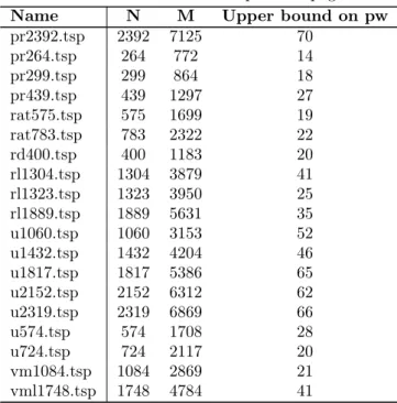
• in Table 8 the upper bounds we have obtained for the Delaunay triangulation of TSP instances we were not able able to solved in 10min.
(a) Increasing number of nodes (b) Increasing number of edges
Figure 4: Computation time for instances of the TreewidthLIB with less than 110 nodes. One dot per instance. The color indicates the density of the instance.
Table 5: Computational results for twl. instance. Name N M pw time(in sec.)
1a8o 64 536 25 0.05
1aac 104 1316 39 0.778
1aba 85 886 28 0.068
1ail 69 631 24 0.03
1awd 89 1080 35 0.239
Name N M pw time(in sec.) 1b67 68 559 16 0.02 1bbz 57 543 25 0.02 1bf4 63 658 26 0.028 1bkf 106 1264 35 0.489 1bkr 107 1340 41 1.813 1brf 49 412 22 0.015 1bx7 41 195 11 0.006 1c4q 67 756 31 0.06 1c5e 95 1148 34 0.218 1c75 69 683 29 0.077 1c9o 66 720 28 0.04 1cc8 70 813 32 0.07 1cka 57 605 27 0.019 1ctj 87 935 32 0.159 1czp 94 1195 36 0.331 1d3b 69 682 25 0.027 1d4t 102 1145 34 0.45 1dj7 73 743 26 0.038 1dp7 76 769 27 0.048 1e0b 60 518 24 0.029 1en2 69 463 16 0.013 1erv 101 1267 38 0.754 1ezg 66 541 23 0.025 1f9m 109 1349 43 5.756 1fjl 65 600 26 0.061 1fk5 85 823 31 0.283 1fr3 67 618 21 0.022 1fse 67 730 26 0.024 1g2b 62 649 28 0.03 1g2r 94 1109 35 0.34 1g6x 52 405 19 0.012 1gcq 68 742 30 0.061 1gut 67 621 22 0.028 1hg7 66 705 28 0.036 1i07 59 397 15 0.011 1i0v 100 1207 38 1.058 1i27 73 747 26 0.036 1i2t 61 644 27 0.022 1ig5 75 816 31 0.1 1igd 61 630 25 0.021 1igq 54 503 23 0.015 1iib 103 1384 38 0.394 1iqz 77 839 31 0.111 1j75 56 558 27 0.024 1jhg 101 841 24 36.55 1jo8 58 608 27 0.022
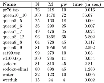
Name N M pw time(in sec.) 1k61 60 581 26 0.029 1kq1 60 607 27 0.026 1kth 52 426 20 0.012 1ku3 61 585 22 0.016 1kw4 67 672 27 0.033 1l9l 70 697 28 0.048 1ldd 74 835 31 0.068 1ljo 74 789 30 0.095 1lkk 103 1162 34 0.588 1mgq 74 798 28 0.042 1oai 58 524 22 0.016 1plc 98 1167 33 0.135 1ptf 87 1137 37 0.261 1pwt 61 657 29 0.034 1qtn 87 788 23 0.072 1r69 63 692 29 0.033 1rb9 48 412 22 0.014 1rro 107 1300 42 3.233 1sem 57 570 26 0.022 1ubq 73 211 12 3.571 BN_28 24 49 5 0.003 BN_29 24 49 5 0.003 alarm 37 65 4 0.004 barley 48 126 7 0.007 david 87 406 13 135.7 eil101.tsp 101 290 11 0.066 eil51.tsp 51 140 8 0.005 eil76.tsp 76 215 11 0.032 fungiuk 15 36 4 0.001 graph03 100 340 21 21.27 graph05 100 416 25 71.24 knights8_8 64 168 16 6.19 kroA100.tsp 100 285 10 0.029 kroB100.tsp 100 284 10 0.025 kroC100.tsp 100 286 10 0.031 kroE100.tsp 100 283 9 0.018 lin105.tsp 105 292 9 0.02 mainuk 48 84 6 0.01 mildew 35 80 5 0.003 myciel3 11 20 5 0.001 myciel4 23 71 10 0.003 myciel5 47 236 20 0.481 oesoca 39 67 4 0.005 oesoca+ 67 208 11 53.39 oesoca42 42 72 4 0.007 pr107.tsp 107 283 7 0.011
Name N M pw time(in sec.) pr76.tsp 76 218 10 0.016 queen10_10 100 1470 72 36.67 queen5_5 25 160 18 0.004 queen6_6 36 290 25 0.007 queen7_7 49 476 35 0.024 queen8_12 96 1368 65 5.802 queen8_8 64 728 45 0.117 queen9_9 81 1056 58 2.592 rat99.tsp 99 279 10 0.03 rd100.tsp 100 286 11 0.054 sodoku 81 810 45 2.81 sodoku-elim1 80 898 45 1.283 water 32 123 10 0.005 weeduk 15 24 4 0.002
Table 6: Upper bounds for twl. instance (10 min. per graph).
Name N M Upper bound on pw
1b0n 103 1011 32 1b0n-006 98 981 32 BN_0 100 300 23 BN_1 100 394 26 BN_10 85 304 23 BN_11 105 631 42 BN_12 90 481 30 BN_2 100 494 32 BN_3 100 451 32 BN_4 100 574 37 BN_7 95 535 35 BN_8 100 420 27 BN_9 105 382 27 celar02 100 311 10 celar06 100 350 11 graph01 100 358 23 huck 74 301 10 jean 77 254 10 myciel6 95 755 38 pathfinder 109 211 7
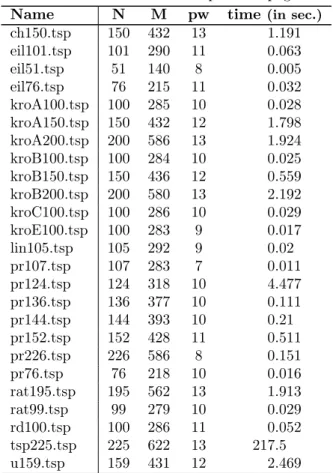
Table 7: Computational results for twl-tsp instance. Name N M pw time(in sec.)
bier127.tsp 127 368 15 3.234
ch130.tsp 130 377 12 0.484
Name N M pw time(in sec.) ch150.tsp 150 432 13 1.191 eil101.tsp 101 290 11 0.063 eil51.tsp 51 140 8 0.005 eil76.tsp 76 215 11 0.032 kroA100.tsp 100 285 10 0.028 kroA150.tsp 150 432 12 1.798 kroA200.tsp 200 586 13 1.924 kroB100.tsp 100 284 10 0.025 kroB150.tsp 150 436 12 0.559 kroB200.tsp 200 580 13 2.192 kroC100.tsp 100 286 10 0.029 kroE100.tsp 100 283 9 0.017 lin105.tsp 105 292 9 0.02 pr107.tsp 107 283 7 0.011 pr124.tsp 124 318 10 4.477 pr136.tsp 136 377 10 0.111 pr144.tsp 144 393 10 0.21 pr152.tsp 152 428 11 0.511 pr226.tsp 226 586 8 0.151 pr76.tsp 76 218 10 0.016 rat195.tsp 195 562 13 1.913 rat99.tsp 99 279 10 0.029 rd100.tsp 100 286 11 0.052 tsp225.tsp 225 622 13 217.5 u159.tsp 159 431 12 2.469
Table 8: Upper bounds for twl-tsp instance (10 min. per graph).
Name N M Upper bound on pw
a280.tsp 280 788 14 d1291.tsp 1291 3845 43 d1655.tsp 1655 4890 40 d198.tsp 198 571 13 d2103.tsp 2103 6290 67 d493.tsp 493 1467 29 d657.tsp 657 1958 27 fl1400.tsp 1400 4138 18 fl1577.tsp 1577 4637 33 fl417.tsp 417 1179 11 gil262.tsp 262 773 19 nrw1379.tsp 1379 4115 39 p654.tsp 654 1806 13 pcb1173.tsp 1173 3501 40 pcb442.tsp 442 1286 20 pr1002.tsp 1002 2972 33