HAL Id: lirmm-00818889
https://hal-lirmm.ccsd.cnrs.fr/lirmm-00818889
Submitted on 29 Apr 2013
HAL is a multi-disciplinary open access
archive for the deposit and dissemination of
sci-entific research documents, whether they are
pub-lished or not. The documents may come from
teaching and research institutions in France or
abroad, or from public or private research centers.
L’archive ouverte pluridisciplinaire HAL, est
destinée au dépôt et à la diffusion de documents
scientifiques de niveau recherche, publiés ou non,
émanant des établissements d’enseignement et de
recherche français ou étrangers, des laboratoires
publics ou privés.
An Efficient Algorithm for Gene/Species Trees
Parsimonious Reconciliation with Losses, Duplications
and Transfers
Jean-Philippe Doyon, Celine Scornavacca, Yu Gorbunov, Gergely Szöllösi,
Vincent Ranwez, Vincent Berry
To cite this version:
Jean-Philippe Doyon, Celine Scornavacca, Yu Gorbunov, Gergely Szöllösi, Vincent Ranwez, et al..
An Efficient Algorithm for Gene/Species Trees Parsimonious Reconciliation with Losses,
Duplica-tions and Transfers. RECOMB-CG: Comparative Genomics, Oct 2010, Ottawa, Canada. pp.93-108,
�10.1007/978-3-642-16181-0_9�. �lirmm-00818889�
An efficient algorithm for gene/species trees
parsimonious reconciliation with losses,
duplications and transfers
Jean-Philippe Doyon1, Celine Scornavacca2, K. Yu. Gorbunov3, Gergely J. Sz¨oll˝osi4, Vincent Ranwez5, and Vincent Berry1
1 LIRMM, CNRS - Univ. Montpellier 2, France. 2 Center for Bioinformatics (ZBIT), Tuebingen Univ., Germany.
3 Kharkevich IITP, Russian Academy of Sciences, Moscow. 4 LBBE, CNRS - Univ. Lyon 1, France.
5 ISEM, CNRS - Univ. Montpellier 2, France.
Abstract. Tree reconciliation methods aim at estimating the evolution-ary events that cause discrepancy between gene trees and species trees. We provide a discrete computational model that considers duplications, transfers and losses of genes. The model yields a fast and exact algorithm to infer time consistent and most parsimonious reconciliations. Then we study the conditions under which parsimony is able to accurately infer such events. Overall, it performs well even under realistic rates, transfers being in general less accurately recovered than duplications. An imple-mentation is freely available at http://www.atgc-montpellier.fr/MPR.
1
Introduction
Duplications, losses and transfers are evolutionary events that shape genomes of eukaryotes and prokaryotes. They result in discrepancies between gene and species trees. Tree reconciliation aims at estimating the course of these events in order to explain the observed incongruences of gene and species trees. A recon-ciliation defines an embedding of a gene tree G into a species tree S, and thus lo-cates duplications, transfers and losses. Reconciliation methods find applications in various areas such as functional annotation in genomics [3], coevolutionary studies in ecology [10], and studies on poputation areas in biogeography.
Probabilistic models have been proposed to reconcile trees [15, 13], but heavy computing times still limit their use to relatively small sets of taxa and small collections of genes. An alternative approach relies on the more tractable com-binatorial principle of parsimony [4]. Yet, with the advent of next generation sequencing technologies, that flood molecular biology with new genomes, even combinatorial methods might become too computationally expensive to han-dle phylogenomic databases, that regularly deal with several dozen thousands of gene families [11]. In this paper, we propose a combinatorial reconciliation method that has the potential to keep pace with new sequencing technologies.
More formally, we consider the Most Parsimonious Reconciliation (MPR) problem: given a species tree S, a gene tree G and respective costs for duplication,
transfer and loss events (respectively denoted D, T, and L events), compute a time-consistent reconciliation that has a minimum cost. Time consistency means that T events happen only horizontally, i.e. between coexisting species, and the cost of a reconciliation is the sum of the costs of the events implied by the embedding of G into S. For instance, when D, T, and L events have cost 5, 10, 1 respectively, the reconciliation of Fig. 1 (left) costs 23.
When only DLS events are considered (S refers to a speciation), the MPR problem can be solved in linear time w.r.t. the size of G for binary trees [17] and remains tractable when S is polytomous [16]. However, when T events are considered, the MPR problem is NP-complete, even for reconciling two binary trees [14]. This strong contrast in complexity is explained by the difficulty of managing the chronological constraints among nodes of S that are induced by T events. When not constraining T events, time inconsistent scenarios can ensue (see Fig. 1; right), as remarked in [14]. These authors solve a variant of the MPR problem with a fast O(|S|2· |G|) algorithm, but that does not handle the time consistency constraints and considers losses a posteriori. A promising approach is to alter the definition of MPR to accept a dated tree S as input [9, 1, 10, 5, 15]. Dates for nodes of S can be obtained by relaxed molecular clock techniques working from gene trees and molecular sequences. Relative dates are sufficient for reconciliation, hence they are little limited by the possible absence of fossil records for the studied species [8]. Given a dated tree S, time consistency can be ensured locally by only considering T events whose donor and receiver branches have intersecting time intervals [10]. However, two locally consistent T events can be globally inconsistent, which then needs to be fixed by altering afterwards the position of the proposed T [10], but this approach does not guarantee to solve MPR exactly. To ensure global consistency, branches of S can be subdivided into time slices transversal to all edges. Then, slices are explored one after the other, and only combinations of T events in a same time slice are considered. This recently led to two exact algorithms, one running in O((|S| · |G|)4) [7] and one claiming a complexity of O(|S|2· |G|) [5, 6].
We propose here a formal modelization that leads to a fast exact algorithm solving the time consistent MPR problem for a dated species tree in O(|S!| · |G|), where S! is a subdivision of S in at most O(|S|2) nodes. Then, we rely on an implementation of this fast algorithm to obtain a first insight for the question:
Is parsimony relevant to infer the true evolutionary scenario of a gene family?
z A B C D x x! x!! y y! a1 b1 c1 d1 u w t1 t2 z A B C D x x! x!! y y! a1 b1 c1 d1 u w t1 t2 t3 t4
Fig. 1: Two scenarios for a gene tree G (plain lines) along a species tree S (tubes), where the symbol ◦ represents loss. (Left) A time consistent scenario. (Right) A scenario that is not time consistent: the transfer from the donor at t3(resp. t4) to a receiver at t1 (resp. t2) implies that u predates (resp. follows) w.
2
Methods
2.1 Basic definitions and notations
Let T be a tree with nodes V (T ) and branches E(T ), and such that only its leaves are labeled. Let r(T ), L(T ), and L (T ) respectively denote its root node, the set of its leaf nodes, and the set of taxa labelling its leaves. We will adopt the convention that the root is at the top of the tree and the leaves at the bottom. An edge of T is denoted (u, v) ∈ E(T ), where u is the parent of v. For a node u of T , Tu denotes the subtree of T rooted at u, up its parent, (up, u) its parent
edge, and T(up,u)denotes the subtree of T rooted at edge (up, u). Given a subset
of leaves K ⊆ L(T ), the homeomorphic tree of T connecting K, denoted TK, is the smallest binary tree induced from T such that L(TK) = K. T is a dated
tree if it is associated with a date function θT : V (T ) → R such that for any two nodes x, x!∈ V (T ), if x! is a strict descendant of x then θ
T(x!) < θT(x). An internal node u of T has one or two children, where {u1} and {u1, u2} respectively denote its child set. It is important to point out that because T is an unordered tree, the children u1 and u2 of u are interchangeable. Given two nodes u, u!of T , u!is said to be a (resp. strict) descendant of u if u is on the path from u!to r(T ) (resp. and u %= u!). An internal node u of T is said to be artificial when it has one and only one child. Contracting an artificial node means that the node is removed from the tree and that its two adjacent edges are merged. A tree T! is said to be a subdivision of a tree T if the recursive contraction of all artificial nodes of T! yields T .
A species tree S is a rooted binary tree such that each element of L (S) represents an extant species labeling exactly one leaf of S (there is a bijection between L(S) and L (S)). A date function θS for S (as defined above) ensures that ∀x ∈ L(S), θS(x) = 0. A gene tree G is a rooted binary tree. From now on, we consider a species tree S and a gene tree G such that L (G) ⊆ L (S) and where L : L(G) → L(S) denotes the function that maps each leaf of G to the unique leaf of S with the same label (leaves of G are labeled with the species from which genes were sampled). To distinguish between G and S, the term edge refers to G and the term branch refers to S.
We introduce below the concept of a scenario describing the evolution of a gene that starts at node r(S) and evolves along S according to DTLS events. Such a scenario generates a completed gene tree denoted Go, whose leaf set is formed of contemporary genes (denoted LC(Go)) but also of lost genes (denoted LL(Go)), see Fig. 1 and 2. Note that L(Go) = LC(Go) ∪ LL(Go).
Definition 1. Given an observed gene tree G and a species tree S, with its time stamp function θS, a DTLS scenario for G along S is denoted (Go, M, θGo),
where Gois a completed gene tree, M : V (Go) → V (S) maps each node of Goto
a node of S, and θGo : V (Go) → [0, θS(r(S))] is a date function that associates
each node of Go to a time stamp of S. The scenario associates a DTLS event to
each node u ∈ V (Go) \ L
C(Go) as described below (where u1 and u2 are the two
1. If u is a leaf of LL(Go), then it corresponds to an L event.
2. If M (u1) = x1, and M (u2) = x2, then u is an S event happening at x in S!.
3. If M (u1) = x and M (u2) = x, then u is a D event along the branch (xp, x).
4. If M (u1) = x, M (u2) = y, and y is neither an ancestor nor a descendant of x, then u is a T event, where (xp, x) and (yp, y) respectively correspond to
the donor and the receiver branches.
A DTLS scenario is said to be consistent if and only if (1) the homeomorphic gene tree Go
LC(Go) is isomorphic to G and (2) for a T event (i.e. Def. 1 (4))
[θS(x), θS(xp)] ∩ [θS(y), θS(yp)] %= ∅.
The cost of such a scenario is denoted Cost(Go, M, θ
Go) = dδ + tτ + lλ,
where d, t, and l respectively denote the number of D, T, and L events, and δ,
τ , and λ are their respective costs.
Consider a species tree S with a time stamp function θS, an observed gene tree G, the leaf-association function L : L(G) → L(S), and costs δ, τ , resp. λ for D, T resp. L events. Given these inputs, the optimization problem considered in the present paper, called MPR, is to compute a consistent DTLS scenario (Go, M, θ
Go) for G along S that minimizes Cost(Go, M, θGo).
2.2 A tractable model of reconciliation
To obtain a tractable model, we discretize time by subdividing the species tree into time slices (similarly as done in [1, 13]), then define a limited number of cases for events to happen, that still allows us to infer a most parsimonious scenario.
Definition 2. (see Fig. 3) Given a species (binary) tree S and a time stamp function θS : V (S) → R, let S! be the subdivision of S constructed as follows:
for each node x ∈ V (S) \ L(S) and each branch (yp, y) ∈ E(S) s.t. θS(yp) > θS(x) > θS(y), an artificial node is inserted along the branch (yp, y) at time θS(x). This subdivision allows us to define a time stamp function θ!S! for S! only
from its topology: for any x ∈ V (S!), θ!
S!(x) is the number of edges separating x
r(G) a1 c1 b1 d1 u w r(Go) a1 c1 b1 d1 u w
Fig. 2: (Left) An observed gene tree G with four leaves a1, b1, c1, and d1, re-spectively belonging to the contemporary species A, B, C, and D (see Fig. 1). (Right) A completed gene tree Go, with L(Go) = L
C(Go) ∪ LL(Go), where LC(Go) = {a1, b1, c1, d1}, and LL(Go) is formed of the three nodes labelled ◦. G is the homeomorphic tree Go
from one of its descendant leaves (which leaf does not matter as they are all at the same distance from x).
The time stamp of a branch (xp, x) of S! is denoted θ!S!(xp, x) = θ!S!(x).
Moreover, for a time t, let Et(S!) = {(xp, x) ∈ E(S!) : θ!S!(xp, x) = t} denote the set of branches of S! located at time t.
Definition 3. Consider a gene tree G and a species tree S with a time stamp function θS, and let S! be the subdivision of S and θ!S! : V (S!) → N be the
corresponding time stamp function. A reconciliation between G and S is denoted
α and maps each edge (up, u) ∈ E(G) onto an ordered sequence of branches of S!, denoted α(up, u), where ℓ denotes its length and αi(up, u) its i-th element for 1 ≤ i ≤ ℓ. Each branch αi(up, u), denoted below (xp, x), respects one and only
one of the following constraints (see Fig. 4).
First, consider the case that (xp, x) is the last branch α!(up, u) of the sequence α(up, u). If u is a leaf of G, then x is the unique leaf of S! that has the same
label as u (that is x = L(u)) (Contemporary taxa mappings). Otherwise, one of the cases below is true.
– {α1(u, u1), α1(u, u2)} = {(x, x1), (x, x2)} (S event); – α1(u, u1) and α1(u, u2) are both equal to (xp, x) (D event); – {α1(u, u1), α1(u, u2)} = {(xp, x), (x!p, x!)}, where (x!p, x!) is any branch of
S! other than (x
p, x) and located at time θ!S!(xp, x) (T event).
If (xp, x) is not the last branch α!(up, u) of the sequence (i.e. i < ℓ), one of
the following cases is true.
– x is an artificial node of S! with a single child x1, and the next branch
αi+1(up, u) is (x, x1) (∅ event);
– x is not artificial and αi+1(up, u) ∈ {(x, x1), (x, x2)} (SL event); – αi+1(up, u) = (x!p, x!) is any branch of S! other than (xp, x) and located at
time θ!
S!(xp, x) (TL event).
A reconciliation α between the gene tree G of Fig. 2 (left) and the subdivision S!of Fig. 3b is depicted in Fig 1(left), where the path α(w, b
1) along S!associated
A B C D
x
y z
(a) A species tree S
A B C D 0 1 2 3 x y z x! x!! y! (b) The subdivision S! of S
Fig. 3: The species tree S and its subdivision S!. The artificial nodes of S! are represented by gray circles and denoted y!, x!, and x!!, where θ!
S!(x) = θ!S!(x!) =
θ!
to the edge (w, b1) is [(y, x!), (y!, x), (x, B)]. Observe that the extended gene tree Go (see Fig. 2; right) is a by-product of the reconciliation α.
Note that T events only happen between branches in a same time slice, hence only time-consistent scenarios are generated by this model. We now argue that the model allows to infer most parsimonious scenarios (see Def. 1). First, note that each loss is coupled with either a speciation (SL) or a transfer (TL). Indeed, any most parsimonious reconciliation embedding G into S! only needs to use a loss when it meets a speciation node of S!where G goes into only one descending tube, or when leaving a tube due to a transfer, with no part of G remaining in the donor tube. Considering a lone loss as a seventh event in Fig. 4 would lead us to examine reconciliations that are not most parsimonious, as this would only allow us to replace – in a Go tree generated by the current model – a single l ∈ LL(Go) by a subtree with no extant species (as the structure of G is common to both these completed gene trees). Such a subtree contains at least two losses and is hence less parsimonious than leaving leaf l in the Go proposed with the current model. Then, any combination of DTLS events resulting from a scenario (Def 1) can be reproduced by the model of Def. 3, safe for combinations that would obviously not lead to most parsimonious scenarios: a speciation of a gene where its two sons go extinct before reaching the leaves of S!; a gene duplication where at least one of its sons goes extinct; a transfer where the transfered gene lineage goes extinct.
Last, note that all cases considered in Def. 3 (see Fig. 4) allow us to progress either in the time slices of S! or along the edges of G. This is because a TL case can not be followed by a second one in a most parsimonious scenario (see Prop. 1 in appendix). Thus, the model offers all ingredients for a dynamic programming algorithm that finds a most parsimonious and time consistent scenario, while still running in time polynomial in |S!| and |G|. In other words, this model allows to solve the MPR problem exactly and in a tractable way.
Note that since the model places each loss immediately after another event (speciation or transfer), it is not able to generate a most parsimonious scenario σ = (Go, M, θo
G) where a lineage is lost after being alive for several slices in a same tube (without meeting a speciation node). However, it can generate a scenario σ! = (Go, ¯M , ¯θo
G) that can be seen as a canonical representative of σ: both scenarios share the same Goand have the same number and localization of D, T, and L events in S (σ and σ! only differ in the position of some L in the
subdivided species tree S!).
2.3 An efficient algorithm to solve MPR
In this section, we propose a polynomial time and space algorithm that uses the tractable reconciliation model of Def. 3 to solve the MPR problem (see Algorithm 1).
Consider an edge (up, u) ∈ E(G), a branch (xp, x) ∈ E(S!), and the time t = θ!
S!(xp, x). Let Cost(u, x) denote the minimal cost over all reconciliations between G(up,u) and the forest of subtrees of S! rooted with a branch located
PS u u2 u1 x1 x2 x xp (a) Speciation (S) u u2 u1 x xp (b) Duplication (D) u u2 u1 x xp x!p x! (c) Transfer (T) u x x1 xp (d) ∅ event u x1 x2 x xp
(e) Speciation + Loss (SL)
u x xp x ! p x! (f) Transfer+Loss (TL)
Fig. 4: The six DTLS events of Def. 3, where an edge (up, u) of Gois mapped onto a branch (xp, x) of the sequence α(up, u). The extended gene tree Gois embedded in the subdivision S! of a species tree S, where an edge of G corresponds to a plain line, a branch of S!corresponds to a dotted tube (white zone), and a node of S! corresponds to a gray zone.
to (up, u) (that is α1(up, u) = (xp, x); see Def. 3). Assuming that the gene tree G and the species tree S are rooted with an artificial branch, Cost(r(G), r(S!)) corresponds to the minimal cost over all reconciliations between G and S. The dynamic programming algorithm (see pseudo-code in Algorithm 1) fills the ma-trix Cost : V (G) × V (S!) → N through two embedded loops: one that visits all edges according to a bottom-up traversal of G and one that visits all time stamps of S! in backward time order (i.e. starting from 0). For the edge (u
p, u) and the time stamp t currently considered (respectively in lines 3 and 4), two consecutive loops over all branches (xp, x) ∈ Et(S!) compute the minimal cost of mapping (up, u) onto (xp, x) according to the six events S, D, T, ∅, SL, and TL (see Fig. 4). For a branch (xp, x) ∈ Et(S!), the first loop (lines 5 to 20) computes the minimal cost among the first five events. TL events can be considered sep-arately (lines 21 to 24) as they may never be immediately followed by a second TL in a most parsimonious scenario (as implied by Property 1 in Appendix). Cost(u, x) is the minimum of the values computed in these two loops.
The case of Fig. 4c is considered at lines 13 to 15 where the cost of a T event starting at (xp, x) is computed for edge (up, u). Assuming that (u, u1) (resp. (u, u2)) is the transfered gene lineage, a subroutine called BestReceiver computes the branch (yp, y) (resp. (zp, z)) that minimizes Cost(u1, y) (resp. Cost(u2, z)) over all branches of S! located at the same time t, other than (x
Algorithm 1Computes Cost(r(G), r(S!)) according to the DTL costs, respec-tively denoted δ, τ , and λ.
1: Construct the subdivision S!of S as described in Def. 2
2: The matrix Cost : V (G) × V (S!) → N is initialized as follows: if u ∈ L(G), x∈ L(S!), and L(u) = x, then Cost(u, x) ← 0. Else, Cost(u, x) ← ∞.
3: for all (up, u) ∈ E(G) according to a bottom-up traversal do
4: for allt∈ {0, 1, . . . , θ!
S!(r(S!))} in backward time order do
5: for allbranch (xp, x) ∈ Et(S!) do
6: if u∈ L(G), x ∈ L(S!), and L(u) = x then
7: Skip lines 8 to 20 and go to the next iteration of the loop at line 5{Base case}
8: Costg← ∞, for each g ∈ {S, D, T, ∅, SL}
9: if uhas two children then 10: if xhas two children then
11: CostS← min{Cost(u1, x1)+Cost(u2, x2), Cost(u1, x2)+Cost(u2, x1)}
12: CostD← Cost(u1, x) + Cost(u2, x) + δ
13: (yp, y) ← BestReceiver((u, u1), t, (xp, x))
14: (zp, z) ← BestReceiver((u, u2), t, (xp, x))
15: CostT← min{ Cost(u1, x) + Cost(u2, z), Cost(u1, y) + Cost(u2, x) } + τ
16: if xhas a single child then 17: Cost∅← Cost(u, x1)
18: if xhas two children then
19: CostSL← min{Cost(u, x1), Cost(u, x2)} + λ
20: Cost(u, x) ← min{Costg : g ∈ {S, D, T, ∅, SL}}
21: for allbranch (xp, x) ∈ Et(S!) do
22: (x!p, x!) ← BestReceiver((up, u), t, (xp, x))
23: CostTL← Cost(u, x!) + τ + λ
24: Cost(u, x) ← min{ Cost(u, x), CostTL}
25: return Cost(r(G), r(S!))
subroutine is used at line 22 for the TL case of Fig. 4f. A similar optimization to compute the optimal receiver for a transfer was found independently in [13]. Algorithm 1 computes the cost of a most parsimonious reconciliation. Back-tracking in the computations of values in the dynamic programming table yields a most parsimonious reconciliation (in the sense of Def. 3), which readily allows to obtain a most parsimonious scenario (see Def. 1), as we argued in Section. 2.2. This algorithm achieves fast running times, in part due to a factorization of the computations of the best receivers (see Appendix for details).
3
Experimental Results
To assess the performance of parsimony, we calculated the most parsimonious reconciliations for a large scale simulated data set that was obtained using a probabilistic model of duplication, transfer, and loss. In our simulations, we started with a single gene at the root of the species tree and generated gene trees according to a Poisson process characterized by rates of duplication, transfer and loss. We compiled two different data sets called ds1 and ds2, aiming both to simulate a relatively large phylogenetic time scale (a bacterial or archean phylum) with realistic loss rates as well as to explore a wide range of duplication and transfer rates. For further details on ds1 and ds2, see the Appendix.
For each data set, we used a single cost per event corresponding to the inverse of the average rate of this event during the simulation process (i.e., for ds1 δ = 1/0.18). According to those costs and for each pair of gene and species trees, we used Algorithm 1 to compute one of the most parsimonious reconciliations denoted αp.
Note that the real reconciliation αR may contain the record of events that cannot be recovered by a reconciliation for G, since no traces of them exist. For instance, subtrees whose leaves are all lost, D events followed straightaway by an Levent, or several TL events in a row. Thus, we post-processed the DTL events of αR, removing hidden parts of αR of the above kinds, but potentially leaving other unrecoverable parts.This leads to obtain a reconciliation α!
R.
We first study under which conditions the parsimony criterion can correctly estimate the DTL events that lead to an observed gene tree G. This can be simply achieved by comparing the costs of the real scenario and that of a most parsimonious one. As soon as the two costs strongly differ, the parsimony is no longer a reasonable approach. Recall that the cost of a reconciliation α can be computed as Cost(α) = dδ + tτ + lλ, where d, t and l are the number of D, resp. T, resp. L implied by α. The relative over cost of α!
Rin terms of parsimony score compared to that of a most parsimonious one is defined below:
OverCost(α!R, αP) =
Cost(α!
R) − Cost(αP)
Cost(αP)
.
Since several most parsimonious scenarios can exist, that Cost(α!
R) = Cost(αP) does not imply αP = α!R. Fig. 5 shows the extent of this over cost depending on the duplication and transfer rates and tree heights. We can see that the over cost is really small for all combinations of duplication and transfer rates we investigated, but does increase with the height of the gene trees. This can be related to hidden events that we failed to identify and remove from α!
R. We now proceed to investigate quantitatively whether parsimony is able to correctly infer the position of DTL events.
Recall that a reconciliation α of a gene tree G defines DTL events associated to internal nodes and edges of G. As the position of duplication and transfer events in Goallow to locate losses, we only focus below on D and T events. Let D(α) ⊆ V (G) \ L(G) denote the subset of internal nodes of G that correspond to a D event and T(α) ⊆ E(G) the subset of edges of G that correspond to a T event. It is important to point out that D(α) and T(α) alone do not resolve where
in S the event has taken place, hence are not sufficient to determine whether a DTLevent is common to two reconciliations. Let DS(α) denote the set of pairs (u, (xp, x)) ∈ D(α) × E(S) such that α places u on the branch (xp, x) of S. Let TS(α) denote the triplet set ((up, u), (xp, x), (yp, y)) ∈ T(α) × E(S)2 such that (up, u) is a T event from the donor (xp, x) to the receiver (yp, y) branches in S. Given a most parsimonious reconciliation αP, its accuracy to retrieve the D and T events of the real (simulated) reconciliation α!
R is evaluated by the ratios of false positive and false negative events defined as follows:
F PE(α!R, αP) = |ES(αP)−ES(α ! R)| |ES(αP)| F NE(α!R, αP) = |ES(α ! R)−ES(αP)| |ES(α!R)| ,
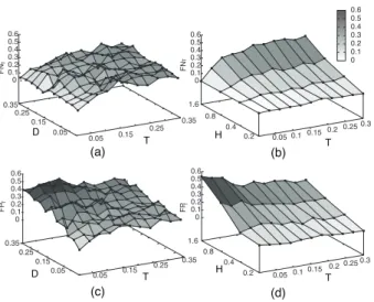
where E = D, T. Figures 6 and 7 show those ratios for various combinations of D, T rates and tree heights.
In Fig. 6, we can see that F PD is close to zero for all combinations of dupli-cation and transfer rates: almost all parsimonious duplidupli-cations are correct (i.e., present in α!
R). The high values of F ND can be explained by several reasons. First, α!
R can contain hidden events that cannot be detected by reconciliation approaches. Second, fixing δ = τ causes the misidentification of some D events replaced by T events in the inference. This would also explain the high ratio of false positive transfers with such rates (see Fig. 7). Finally, this can be due to the wrong most parsimonious reconciliation proposed among the several possible ones. This also explains the quite high level of false negatives for T events.
4
Conclusion
We presented a new model for reconciling gene and species trees. This model leads to a fast and exact algorithm to compute a time consistent and most par-simonious reconciliation while accounting for duplications, losses and transfers. Simulations showed that the parsimony criterion performs satisfactorily under realistic conditions at the phylum level. At the inter-phlyum level, transfers are
0 0.1 0.2 0.3 0.4 0.5 0.6 0.05 0.1 0.15 0.2 0.25 0.3 0.2 0.4 0.8 1.6 0 0.1 0.2 0.3 0.4 0.5 0.6 T H 0.05 0.15 0.25 0.35 0.05 0.15 0.25 0.35 0 0.1 0.2 0.3 0.4 0.5 0.6 over cost T D (a) (b) over cost
Fig. 5: Over cost of simulated scenarios compared to that of most parsimonious ones for combinations of heights, transfer and duplication rates, i.e. ds1(a) and ds2 (b). High values show cases where parsimony criterion is inadequate.
0.05 0.1 0.15 0.2 0.25 0.3 0.2 0.4 0.8 1.6 0 0.1 0.2 0.3 0.4 0.5 0.6 FN D T H 0 0.1 0.2 0.3 0.4 0.5 0.6 0.05 0.1 0.15 0.2 0.25 0.3 0.2 0.4 0.8 1.6 0 0.1 0.2 0.3 0.4 0.5 0.6 FP D T H 0.05 0.15 0.25 0.35 0.05 0.15 0.25 0.35 0 0.1 0.2 0.3 0.4 0.5 0.6 FP D T D 0.05 0.15 0.25 0.35 0.05 0.15 0.25 0.35 0 0.1 0.2 0.3 0.4 0.5 0.6 FN D T D (a) (b) (c) (d)
Fig. 6: Accuracy of parsimony to estimate reconciliations: ratios of false negative (a,b) and false positive (c,d) to estimate and localize D events, for combinations of heights, transfer and duplication rates, i.e. ds1(a,c) and ds2 (b,d).
(a) (b) (c) (d) 0.05 0.15 0.25 0.35 0.05 0.15 0.25 0.35 0 0.1 0.2 0.3 0.4 0.5 0.6 FN T T D 0.05 0.15 0.25 0.35 0.05 0.15 0.25 0.35 0 0.1 0.2 0.3 0.4 0.5 0.6 FP T T D 0.05 0.1 0.15 0.2 0.25 0.3 0.2 0.4 0.8 1.6 0 0.1 0.2 0.3 0.4 0.5 0.6 0 0.1 0.2 0.3 0.4 0.5 0.6 T H T FN T FP 0.05 0.1 0.15 0.2 0.25 0.3 0.2 0.4 0.8 1.6 0 0.1 0.2 0.3 0.4 0.5 0.6 T H
Fig. 7: Accuracy of parsimony to estimate reconciliations: ratios of false negative (a,b) and false positive (c,d) to estimate and localize T events, for combinations of heights, transfer and duplication rates, i.e. ds1(a,c) and ds2 (b,d).
more difficult to recover and the existence of several most-parsimonious reconcil-iations might be a decisive factor there. This needs further scrutiny. Moreover, running times are on average 1.09s (resp. 1.38s) for low (resp. high) rates of events for trees on 100 species. This clearly scales the reconciliation approach up to the phylogenomic stage, where several tens of thousand genes are considered. Many things remain to be done, among others to allow for multifurcating gene and species trees and to measure the accuracy of the reconciliation approach for orthology prediction (where the localization of events is not needed, increasing the accuracy of the method w.r.t. our results) compared to other methods.
References
1. C. Conow, D. Fielder, Y. Ovadia, and R. Libeskind-Hadas. Jane: a new tool for the cophylogeny reconstruction problem. Algorithms Mol Biol, 5:16, 2010.
2. M. Csuros and I. Miklos. Streamlining and Large Ancestral Genomes in Archaea Inferred with a Phylogenetic Birth-and-Death Model. Mol Biol Evol, 26(9):2087–2095, 2009. 3. Toni Gabaldon. Computational approaches for the prediction of protein function in the
mitochondrion. Am J Physiol Cell Physiol, 291(6):C1121–1128, 2006.
4. M. Goodman, J. Czelusniak, G. W. Moore, Romero A. Herrera, and G. Matsuda. Fitting the gene lineage into its species lineage, a parsimony strategy illustrated by cladograms constructed from globin sequences. Syst. Zool., 28:132–163, 1979.
5. K. Yu. Gorbunov and V. A. Lyubetsky. Reconstructing genes evolution along a species tree. Mol. Biol. (Mosk.), 43:946–958, 2009.
6. K. Yu. Gorbunov and V. A. Lyubetsky. An algorithm of reconciliation of gene and species trees and inferring gene duplications, losses and horizontal transfers. Information pro-cesses, 10(2):140–144, 2010. (In Russian).
7. R. Libeskind-Hadas and M. A. Charleston. On the computational complexity of the reticulate cophylogeny reconstruction problem. JCB, 16(1):105–117, 2009.
8. S.P. Loader, D. Pisani, J.A. Cotton, D.J. Gower, J.J. Day, and M. Wilkinson. Relative time scales reveal multiple origins of parallel disjunct distributions of african caecilian amphibians. Biol Lett., pp. 505–508, October 2007.
9. D. Merkle and M. Middendorf. Reconstruction of the cophylogenetic history of related phylogenetic trees with divergence timing information. Theory Biosci, 123(4):277–299, 2005.
10. D. Merkle, M. Middendorf, and N. Wieseke. A parameter-adaptive dynamic programming approach for inferring cophylogenies. BMC Bioinformatics, 11(Suppl 1):S60, 2010. 11. S. Penel, A. M. Arigon, J. F. Dufayard, A. S. Sertier, V. Daubin, L. Duret, M. Gouy,
and G. Perriere. Databases of homologous gene families for comparative genomics. BMC Bioinformatics, 10 Suppl 6:S3, 2009.
12. A. Rambaut. Phylogen: phylogenetic tree simulator package, 2002.
13. A. Tofigh. Using Trees to Capture Reticulate Evolution, Lateral Gene Transfers and Cancer Progression. PhD thesis, KTH Royal Institute of Technology, Sweden, 2009. 14. A. Tofigh, M. Hallett, and J. Lagergren. Simultaneous identification of duplications and
lateral gene transfers. IEEE/ACM TCBB, 99, 2010.
15. A. Tofigh, J. Sj¨ostrand, B. Sennblad, L. Arvestad, and J. Lagergren. Detecting LGTs
using a novel probabilistic model integrating duplications, lgts, losses, rate variation, and sequence evolution, Manuscript.
16. B. Vernot, M. Stolzer, A. Goldman, and D. Durand. Reconciliation with non-binary species trees. J. Comput. Biol., 15:981–1006, 2008.
17. L. Zhang. On a mirkin-muchnik-smith conjecture for comparing molecular phylogenies. Journal of Computational Biology, 4(2):177–187, 1997.
A
Some proofs
Property 1. Consider a parsimonious reconciliation α between G and S, an edge
(up, u) of G and a time t. The sequence α(up, u) contains at most two branches of S! located at time t. If there are two such branches denoted α
i(up, u) and αj(up, u), then they are adjacent in the sequence α(up, u) (i.e. |i − j| = 1). Proof The adjacency of the two branches follows immediately from Def. 3 (relying on the fact that both happen at time t).
Assume that α contains two TL events for (up, u) described as follows: there are three adjacent branches αi(up, u), αi+1(up, u) and αi+2(up, u) in Et(S!), which respectively corresponds (according to Def. 3) to the donor of the first TLevent, the receiver (resp. donor) of the first (resp. second) TL event, and the receiver of the second TL event.
As the cost of a single TL event between αi(up, u) and αi+2(up, u) is smaller than the cost for the previous two TL events, α is not a parsimonious
reconcili-ation. !
Proof of the complexity of the algorithm
Proof of the time complexity. We claim the algorithm runs in O(n!m) where n! is the size of the subdivides species tree S! and m is the size of G.
The loop over the edges of G (line 3) runs for Θ(m) iterations. The loop over the times t of S! (line 4) together with the two loops over branches E
t(S!) in sequence (line 5 and 21) run for Θ(n!) iterations. Thus, lines 6 to 20 and lines 22 to 24 are run Θ(n!m) time globally. For the nodes u ∈ V (G) and x ∈ V (S!) currently visited, we now have to prove that Cost(u, x) can be computed in constant time, which is obviously the case for the cost associated to the S, D, ∅, and SL events (see lines 11, 12, 16, and 18, respectively). We prove below how the cost associated to a T event (lines 13 to 15) can be computed in constant time, considering that both genes are conserved (we omit the case for a TL combination at lines 22 to 24, as it is solved using the same optimization idea). Consider a T event from a donor (xp, x) ∈ Et(S!), assuming w.l.o.g. that (u, u1) is conserved in the lineage (xp, x) while (u, u2) is transfered. The algo-rithm needs to compute the optimal receiver (i.e. that leading to a minimum cost) for (u, u2) in Et(S!) \ {(xp, x)}. As currently stated, i.e. in the most read-able form, Algorithm 1 allows to compute the best receiver in Θ(|Et(S!)|) time by a simple loop over the branch set Et(S!) (line 14; subroutine BestReceiver). However, slightly modifying the statement of the algorithm allows to compute the best receiver in constant time at line 14 (and similarly lines 13 and 22). To achieve this, immediately before the loop over the branch set Et(S!) (line 5), add another loop on Et(S!) to find the first and second optimal receivers for (u, u2) in Et(S!) and denote (x!p, x!) and (x!!p, x!!) these respective receivers. Second, when a donor (xp, x) ∈ Et(S!) is visited during the loop at line 5, the optimal receiver for (u, u2) in Et(S!) \ {(xp, x)} is the first optimal receiver if
(xp, x) %= (x!p, x!), and the second one otherwise. Hence line 13 now requires con-stant time, while adding the additional loop mentioned above doesn’t cost more than the already existing loop of line 5. As a result, the overall time complexity of the algorithm is in Θ(n!m). Note that [13] independently uses a similar idea to obtain a fast reconciliation algorithm.
Proof of the space complexity. The size of the whole matrix Cost(u, x) is in Θ(n!m), all other variables used in the algorithm are constant in size, and the
space complexity is then immediate. !
Sketch of the proof for the correctness of the algorithm
Given a tree T , define the height of a node u ∈ V (T ), denoted h(u), as the length of the unique path from u to r(T ), and the height of T , denoted h(T ), is the maximal height over all its nodes.
Consider the edge (up, u) and the time stamp t examined at an iteration of the main loops (respectively in lines 3 and 4) in the algorithm. For any branch (xp, x) ∈ Et(S!), we now explain how the two loops compute Cost(u, x) by considering all six events seperately. First, for the S and D events (lines 11 and 12 resp.), the consistency of the corresponding cost is ensured because for any child u! ∈ {u1, u2} and any branch (x!
p, x!) of S!, Cost(u!, x!) is previously computed during the bottom-up traversal of G. Second, for the ∅ and SL events (lines 17 and 19 resp.), the optimality is verified because for any branch (x!
p, x!) ∈ Et−1(S!), Cost(u, x!) is computed during the iteration for the time (t − 1) of S!. The cases for the T and TL events use the optimal receivers for (up, u) and its two descendant edges, all located at time t. The bottom-up traversal of G im-plies that Cost(u!, x!) is computed for all children u!∈ {u
1, u2} and all branches (x!
p, x!) ∈ Et(S!). Thus, for a donor (xp, x) ∈ Et(S!), BestReceiver ((u!
p, u!), t, (xp, x)) computes (in linear time in the size of Et(S!)) the best re-ceiver for the transfered edge (u!
p, u!). For the two descendant edges (u, u1) and (u, u2), the best receiver are respectively computed at lines line 13 and 14. For a Tevent (line 15) with (xp, x) as the donor, the consistency of the corresponding cost is ensured following the same reasons as for a D event together with the availability of these two best receivers.
Considering a TL event with (xp, x) as the donor, Property 1 implies that the minimal cost of mapping (up, u) onto an optimal receiver (x!p, x!) ∈ Et(S!) \ {(xp, x)} corresponds to any of the five events considered in the third loop (line 5). Thus, when BestReceiver computes such an optimal receiver (line 22), its optimality is ensured together with that for the cost of a TL event (line 23) and the final cost (line 24).
This conclude the sketch to prove the correctness of Algorithm 1. Moreover, it is important to point out that a scenario in which a node u ∈ V (G) has its two descendant edges (u, u1) and (u, u2) both transfered is implicitly considered by our combinatorial model of reconciliations. Indeed, given u ∈ V (G) and a branch (xp, x) ∈ Et(S!) that is the last one of the sequence α(up, u), assume that this association corresponds to a T event for u, where u1 is conserved by
the donor (xp, x) and u2 is given to a receiver (see T event in Def. 3). Given that the first branch α1(u, u1) equals (xp, x) in the sequence associated to u1, a reconciliation allows the next branch of this sequence (i.e. α2(u, u1)) to be any branch in Et(S!) \ {(xp, x)} (see TL event in Def. 3).
B
Simulated data sets
B.1 Simulated species trees
We generated a sets of 10 random ultrametric species trees with 100 species using a standard birth death process with PhyloGen [12] (the ratio of birth to death rate was 1.25). All species trees were normalized to a common height h, with time measured from the leaves of the species tree at t = 0 to its root at t = h. The time order of the internal nodes (speciation events), and hence S, was uniquely determined by the branch lengths of the tree.
B.2 Simulated DTL scenarios
Starting with a single gene at time t = h at the root of S, we generated evolu-tionary scenarios according to a Poisson process characterized by rates of dupli-cation, transfer and loss. At time t, each extant gene underwent duplication with rate rδ or loss at rate rλ. Transfers to each branch of the species tree at time t occurred at rate rτ, with the donor gene drawn uniformly from genes extant at time t except the branch considered.
Instances of the above Poisson process correspond to a completed gene tree Goand a simulated reconciliation, denoted α
R, that includes a complete record of the DTLS events that gave rise to it. The gene tree G, obtained from Go by removing the extinct subtrees of Go, is used as the input to the parsimony algorithm.
Cs˝ur¨os and Mikl´os recently provided estimates of the relative magnitude of duplication, transfer and loss rates in the domain of Archaea. For our purposes, there results can be summarized by the average ratio of 23% duplication, 1% gain, and 76% loss, and an approximate loss rate of 1.5 (assuming a tree with unit height). As many transfer scenarios do not leave behind a clear signal in the phylogenetic profile of a gene family, the gain rate can potentially underestimates the rate of transfer and overestimates the rate of duplication.
To explore a wide as possible set of parameters we chose two different ways of varying the rates of duplication, transfer, and loss.
In the first data set, denoted ds1, we chose a fixed loss rate of rλ = 0.7 (with tree height h = 1) and varied values of both rδ and rτin the interval [0.01, 0.35], choosing 11 values of each parameter, resulting in 11 × 11 sets of rates. This choice of parameters aims to simulate a relatively large phylogenetic time scale, corresponding to, e.g. a bacterial or archean phylum, with realistic loss rates, while making no assumption about the ratio of transfer and loss events, and only requiring rδ+ rτ ≤ rλ. We generated 5 gene trees per species tree and per parameter set (6,050 in total).
In the second data set, denoted by ds2, we chose to fix the ratio of rδ+ rτ to rλ as follows: rλ/(rδ+ rτ + rλ) = 0.7 (motivated by the results of Cs˝ur¨os and Mikl´os [2]). This choice of parameters aims at investigating the accuracy of parsimony on different phylogenetic scales, using 4 different tree heights h = 0.2, 0.4, 0.8 and 1.6. We varied the transfer rate rτ ∈ [0, 0.3] in 11 steps (with consequently rδ = 0.3 − rτ). We generated 20 gene trees, per species tree and per rate parameter set (8,800 in total).
C
Complementary experimental results
In some context, such as sequence orthology prediction, only the tagging of the nodes of G is important. Thus another way to account for errors is to compare the tagging inferred by a parsimony reconciliation with the tagging due to the real scenario. Fig. 8 shows error ratios when false positive and negative are judged on the fact that the internal nodes of the gene tree are assigned to the correct event they represent in the simulated scenario (i.e. one of DTLS). It can be noted that both error levels for transfers decrease remarkably when accounting for transfers in this way (compare with Fig. 7).
(a) (b) (c) (d) 0 0.1 0.2 0.3 0.4 0.5 0.6 0.05 0.15 0.25 0.35 0.05 0.15 0.25 0.35 0 0.1 0.2 0.3 0.4 0.5 0.6 FP T T D 0.05 0.15 0.25 0.35 0.05 0.15 0.25 0.35 0 0.1 0.2 0.3 0.4 0.5 0.6 FN T T D 0.05 0.1 0.15 0.2 0.25 0.3 0.2 0.4 0.8 1.6 0 0.1 0.2 0.3 0.4 0.5 0.6 FP T T H 0.05 0.1 0.15 0.2 0.25 0.3 0.2 0.4 0.8 1.6 0 0.1 0.2 0.3 0.4 0.5 0.6 FN T T H
Fig. 8: Ratios of false negative (a-b) and false positive (c-d) for T events, for various combinations of heights, transfer and duplication rates, i.e. ds1 (a-c) and ds2(b-d) when considering a transfer to be common to αR! and αP as soon
as the same branch of G is transferred, i.e., without looking at place where the receiver is in S.