Common gardens in teosintes reveal the establishment of a syndrome of adaptation to altitude

HAL Id: hal-02345676

https://hal.archives-ouvertes.fr/hal-02345676

Preprint submitted on 7 Nov 2019

HAL is a multi-disciplinary open access

archive for the deposit and dissemination of sci-entific research documents, whether they are pub-lished or not. The documents may come from teaching and research institutions in France or abroad, or from public or private research centers.

L’archive ouverte pluridisciplinaire HAL, est destinée au dépôt et à la diffusion de documents scientifiques de niveau recherche, publiés ou non, émanant des établissements d’enseignement et de recherche français ou étrangers, des laboratoires publics ou privés.

Distributed under a Creative Commons Attribution - NonCommercial - NoDerivatives| 4.0 International License

Margaux-Alison Fustier, Natalia Elena, Martinez-Ainsworth Jonas, Andres

Aguirre-Liguori, Juliette Meaux, M-A Fustier, N Martínez-Ainsworth, J

Aguirre-Liguori, Anthony Venon, Hélène Corti, et al.

To cite this version:

Margaux-Alison Fustier, Natalia Elena, Martinez-Ainsworth Jonas, Andres Aguirre-Liguori, Juliette Meaux, et al.. Common gardens in teosintes reveal the establishment of a syndrome of adaptation to altitude. 2019. �hal-02345676�

Title:

Short Title

M-A. Fustier1, ☯, N.E. Martínez-Ainsworth1, ☯, J.A. Aguirre-Liguori2, A. Venon1, H. Corti1, A. Rousselet1, F. Dumas1, H. Dittberner3, M.G. Camarena4, D. Grimanelli5,O. Ovaskainen6,7, M. Falque1, L. Moreau1, J. de Meaux3, S. Montes4, L.E. Eguiarte2, Y. Vigouroux5, D. Manicacci1,*, M.I. Tenaillon1,*

1

: Génétique Quantitative et Evolution – Le Moulon, Institut National de la Recherche Agronomique, Université Paris-Sud, Centre National de la Recherche Scientifique, AgroParisTech, Université Paris-Saclay, France

2

: Departamento de Ecología Evolutiva, Instituto de Ecología, Universidad Nacional Autónoma de México, Ciudad de México, Mexico

3

: Institute of Botany, University of Cologne Biocenter, 47b Cologne, Germany

4

: Campo Experimental Bajío, Instituto Nacional de Investigaciones Forestales, Agrícolas y Pecuarias, Celaya, Mexico

5

: Université de Montpellier, Institut de Recherche pour le développement, UMR Diversité, Adaptation et Développement des plantes, Montpellier, France

6

: Organismal and Evolutionary Biology Research Programme, PO Box, 65, FI-00014 University of Helsinki, Finland

7

: Centre for Biodiversity Dynamics, Department of Biology, Norwegian University of Science and Technology, N-7491 Trondheim, Norway

☯_{: The authors equally contributed to this work}

* co-corresponding authors

Abstract

1 2

In plants, local adaptation across species range is frequent. Yet, much has to 3

be discovered on its environmental drivers, the underlying functional traits and their 4

molecular determinants. Genome scans are popular to uncover outlier loci potentially 5

involved in the genetic architecture of local adaptation, however links between 6

outliers and phenotypic variation are rarely addressed. Here we focused on adaptation 7

of teosinte populations along two elevation gradients in Mexico that display 8

continuous environmental changes at a short geographical scale. We used two 9

common gardens, and phenotyped 18 traits in 1664 plants from 11 populations of 10

annual teosintes. In parallel, we genotyped these plants for 38 microsatellite markers 11

as well as for 171 outlier single nucleotide polymorphisms (SNPs) that displayed 12

excess of allele differentiation between pairs of lowland and highland populations 13

and/or correlation with environmental variables. Our results revealed that phenotypic 14

differentiation at 10 out of the 18 traits was driven by local selection. Trait covariation 15

along the elevation gradient indicated that adaptation to altitude results from the 16

assembly of multiple co-adapted traits into a complex syndrome: as elevation 17

increases, plants flower earlier, produce less tillers, display lower stomata density and 18

carry larger, longer and heavier grains. The proportion of outlier SNPs associating 19

with phenotypic variation, however, largely depended on whether we considered a 20

neutral structure with 5 genetic groups (73.7%) or 11 populations (13.5%), indicating 21

that population stratification greatly affected our results. Finally, chromosomal 22

inversions were enriched for both SNPs whose allele frequencies shifted along 23

elevation as well as phenotypically-associated SNPs. Altogether, our results are 24

consistent with the establishment of an altitudinal syndrome promoted by local 25

selective forces in teosinte populations in spite of detectable gene flow. Because 26

elevation mimics climate change through space, SNPs that we found underlying 27

phenotypic variation at adaptive traits may be relevant for future maize breeding. 28

29

Keywords:

F

30

syndrome; pleiotropy; chromosomal inversions. 31

32

Author summary

33

Across their native range species encounter a diversity of habitats promoting local 34

adaptation of geographically distributed populations. While local adaptation is 35

widespread, much has yet to be discovered about the conditions of its emergence, the 36

targeted traits, their molecular determinants and the underlying ecological drivers. 37

Here we employed a reverse ecology approach, combining phenotypes and genotypes, 38

to mine the determinants of local adaptation of teosinte populations distributed along 39

two steep altitudinal gradients in Mexico. Evaluation of 11 populations in two 40

common gardens located at mid-elevation pointed to adaptation via an altitudinal 41

multivariate syndrome, in spite of gene flow. We scanned genomes to identify loci 42

with allele frequencies shifts along elevation, a subset of which associated to trait 43

variation. Because elevation mimics climate change through space, these 44

polymorphisms may be relevant for future maize breeding. 45

Introduction

46 47

Local adaptation is key for the preservation of ecologically useful genetic 48

variation [1]. The conditions for its emergence and maintenance have been the focus 49

of a long-standing debate nourished by ample theoretical work [2-9]. On the one 50

hand, spatially-varying selection promotes the evolution of local adaptation, provided 51

that there is genetic diversity underlying the variance of fitness-related traits [10]. On 52

the other hand, opposing forces such as neutral genetic drift, temporal fluctuations of 53

natural selection, recurrent introduction of maladaptive alleles via migration and 54

homogenizing gene flow may hamper local adaptation (reviewed in [11]) . Meta-55

analyzes indicate that local adaptation is pervasive in plants, with evidence of native-56

site fitness advantage in reciprocal transplants detected in 45% to 71% of populations 57

[12, 13]. 58

While local adaptation is widespread, much has yet to be discovered about the 59

traits affected by spatially-varying selection, their molecular determinants and the 60

underlying ecological drivers [14]. Local adaptation is predicted to increase with 61

phenotypic, genotypic and environmental divergence among populations [6, 15, 16]. 62

Comparisons of the quantitative genetic divergence of a trait (QST) with the neutral 63

genetic differentiation (FST) can provide hints on whether trait divergence is driven by 64

spatially-divergent selection [17-20]. Striking examples of divergent selection include 65

developmental rate in the common toad [21], drought and frost tolerance in alpine 66

populations of the European silver fir [22], and traits related to plant phenology, size 67

and floral display among populations of Helianthus species [23, 24]. These studies 68

have reported covariation of physiological, morphological and/or life-history traits 69

across environmental gradients which collectively define adaptive syndromes. Such 70

syndromes may result from several non-exclusive mechanisms: plastic responses, 71

pleiotropy, non-adaptive genetic correlations among traits (constraints), and joint 72

selection of traits encoded by different sets of genes resulting in adaptive correlations. 73

In some cases, the latter mechanism may involve selection and rapid spread of 74

chromosomal inversions that happen to capture multiple locally favored alleles [25] as 75

exemplified in Mimulus guttatus [26]. While distinction between these mechanisms is 76

key to decipher the evolvability of traits, empirical data on the genetic bases of 77

correlated traits are currently lacking [27]. 78

The genes mediating local adaptation are usually revealed by genomic regions 79

harboring population-specific signatures of selection. These signatures include alleles 80

displaying greater-than-expected differentiation among populations [28] and can be 81

identified through FST-scans [29-35]. However, FST-scans and its derivative methods 82

[28] suffer from a number of limitations, among them a high number of false positives 83

(reviewed in [36, 37]) and the lack of power to detect true positives [38]. Despite 84

these caveats, FST-outlier approaches have helped in the discovery of emblematic 85

adaptive alleles such as those segregating at the EPAS1 locus in Tibetan human 86

populations adapted to high altitude [39]. An alternative to detect locally adaptive loci 87

is to test for genotype-environment correlations [35, 40-45]. Correlation-based 88

methods can be more powerful than differentiation-based methods [46], but spatial 89

autocorrelation of population structure and environmental variables can lead to 90

spurious signatures of selection [47]. 91

Ultimately, to identify the outlier loci that have truly contributed to improve 92

local fitness, a link between outliers and phenotypic variation needs to be established. 93

The most common approach is to undertake association mapping. However, recent 94

literature in humans has questioned our ability to control for sample stratification in 95

such approach [48]. Detecting polymorphisms responsible for trait variation is 96

particularly challenging when trait variation and demographic history follow parallel 97

environmental (geographic) clines. Plants however benefit from the possibility of 98

conducting replicated phenotypic measurements in common gardens, where 99

environmental variation is controlled. Hence association mapping has been 100

successfully employed in the model plant species Arabidopsis thaliana, where 101

broadly distributed ecotypes evaluated in replicated common gardens have shown that 102

fitness-associated alleles display geographic and climatic patterns indicative of 103

selection [49]. Furthermore, the relative fitness of A. thaliana ecotypes in a given 104

environment could be predicted from climate-associated SNPs [50]. While climatic 105

selection over broad latitudinal scales produces genomic and phenotypic patterns of 106

local adaptation in the selfer plant A. thaliana, whether similar patterns exist at shorter 107

spatial scale in outcrossing species remains to be elucidated. 108

We focused here on a well-established outcrossing plant system, the teosintes, 109

to investigate the relationship of molecular, environmental, and phenotypic variation 110

in populations sampled across two elevation gradients in Mexico. The gradients 111

covered a relatively short yet climatically diverse, spatial scale. They encompassed 112

populations of two teosinte subspecies that are the closest wild relatives of maize, Zea 113

mays ssp. parviglumis (hereafter parviglumis) and Z. mays ssp. mexicana (hereafter 114

mexicana). The two subspecies display large effective population sizes [51], and span 115

a diversity of climatic conditions, from warm and mesic conditions below 1800 m for 116

parviglumis, to drier and cooler conditions up to 3000 m for mexicana [52]. Previous 117

studies have discovered potential determinants of local adaptation in these systems. 118

At a genome-wide scale, decrease in genome size correlates with increasing altitude, 119

which likely results from the action of natural selection on life cycle duration [53, 54]. 120

More modest structural changes include megabase-scale inversions that harbor 121

clusters of SNPs whose frequencies are associated with environmental variation [55, 122

56]. Also, differentiation- and correlation-based genome scans in teosinte populations 123

succeeded in finding outlier SNPs potentially involved in local adaptation [57, 58]. 124

But a link with phenotypic variation has yet to be established. 125

In this paper, we genotyped a subset of these outlier SNPs on a broad sample 126

of 28 teosinte populations, for which a set of neutral SNPs was also available; as well 127

as on an association panel encompassing 11 populations. We set up common gardens 128

in two locations to evaluate the association panel for 18 phenotypic traits over two 129

consecutive years. Individuals from this association panel were also genotyped at 38 130

microsatellite markers to enable associating genotypic to phenotypic variation while 131

controlling for sample structure and kinship among individuals. We addressed three 132

main questions: What is the extent of phenotypic variation within and among 133

populations? Can we define a set of locally-selected traits that constitute a syndrome 134

of adaptation to altitude? What are the genetic bases of such syndrome? We further 135

discuss the challenges of detecting phenotypically-associated SNPs when trait and 136

genetic differentiation parallel environmental clines. 137

138

Results

139 140

Trait-by-trait analysis of phenotypic variation within and among populations.

141

In order to investigate phenotypic variation, we set up two common garden 142

experiments located in Mexico to evaluate individuals from 11 teosinte populations 143

(Fig 1). The two experimental fields were chosen because they were located at 144

intermediate altitudes (S1 Fig). Although natural teosinte populations are not typically 145

encountered around these locations [52], we verified that environmental conditions 146

were compatible with both subspecies (S2 Fig). The 11 populations were sampled 147

among 37 populations (S1 Table) distributed along two altitudinal gradients that range 148

from 504 to 2176 m in altitude over ~460 kms for gradient a, and from 342 to 2581m 149

in altitude over ~350 kms for gradient b (S1 Fig). Lowland populations of the 150

subspecies parviglumis (n=8) and highland populations of the subspecies mexicana 151

(n=3) were climatically contrasted as can be appreciated in the Principal Component 152

Analysis (PCA) computed on 19 environmental variables (S2 Fig). The corresponding 153

set of individuals grown from seeds sampled from the 11 populations formed the 154

association panel. 155

156

Figure 1. Geographical location of sampled populations and experimental fields.

157

The entire set of 37 Mexican teosinte populations is shown with parviglumis (circles) 158

and mexicana (triangles) populations sampled along gradient a (white) and gradient b 159

(black). The 11 populations indicated with a purple outline constituted the association 160

panel. This panel was evaluated in a four-block design over two years in two 161

experimental fields located at mid-elevation, SENGUA and CEBAJ. Two major cities 162

(Mexico City and Guadalajara) are also indicated. Topographic surfaces have been 163

obtained from International Centre for Tropical Agriculture (Jarvis A., H.I. Reuter, A. 164

Nelson, E. Guevara, 2008, Hole-filled seamless SRTM data V4, International Centre 165

for Tropical Agriculture (CIAT), available from http://srtm.csi.cgiar.org). 166

167

We gathered phenotypic data during two consecutive years (2013 and 2014). 168

We targeted 18 phenotypic traits that included six traits related to plant architecture, 169

three traits related to leaves, three traits related to reproduction, five traits related to 170

grains, and one trait related to stomata (S2 Table). Each of the four experimental 171

assays (year-field combinations) encompassed four blocks. In each block, we 172

evaluated one offspring (half-sibs) of ~15 mother plants from each of the 11 teosinte 173

populations using a semi-randomized design. After filtering for missing data, the 174

association panel included 1664 teosinte individuals. We found significant effects of 175

Field, Year and/or their interaction for most traits, and a highly significant Population 176

effect for all of them (model M1, S3 Table). 177

We investigated the influence of altitude on each trait independently. All traits, 178

except for the number of nodes with ears (NoE), exhibited a significant effect of 179

altitude (S3 Table, M3 model). Note that after accounting for elevation, the 180

population effect remained significant for all traits, suggesting that factors other than 181

altitude contributed to shape phenotypic variation among populations. Traits related to 182

flowering time and tillering displayed a continuous decrease with elevation, and traits 183

related to grain size increased with elevation (Fig 2 & S3 Fig). Stomata density also 184

diminished with altitude (Fig 2). In contrast, plant height, height of the highest ear, 185

number of nodes with ear in the main tiller displayed maximum values at intermediate 186

altitudes (highland parviglumis and lowland mexicana) (S3 Fig). 187

We estimated narrow-sense heritabilites (additive genotypic effect) per 188

population for all traits using a mixed animal model. Average per-trait heritability 189

ranged from 0.150 for tassel branching to 0.664 for female flowering time, albeit with 190

large standard errors (S2 Table). We obtained higher heritability for grain related 191

traits when mother plant measurements were included in the model with 0.631 (sd = 192

0.246), 0.511 (sd = 0.043) and 0.274 (sd = 0.160) for grain length, weight and width, 193

respectively, suggesting that heritability was under-estimated for other traits where 194

mother plant values were not available. 195

Figure 2: Population-level box-plots of adjusted means for four traits. Traits are

197

female flowering time (A), male flowering time (B), grain length (C) and stomata 198

density (D). Populations are ranked by altitude. Parviglumis populations are shown in 199

green and mexicana in red, lighter colors are used for gradient ‘a’ and darker colors 200

for gradient ‘b’. In the case of male and female flowering time, we report data for 9 201

out of 11 populations because most individuals from the two lowland populations 202

(P1a and P1b) did not flower in our common gardens. Covariation with elevation was 203

significant for the four traits. Corrections for experimental setting are detailed in the 204

material and methods section (Model M’1). 205

206

Multivariate analysis of phenotypic variation and correlation between traits.

207

Principal component analysis including all phenotypic measurements 208

highlighted that 21.26% of the phenotypic variation scaled along PC1 (Fig 3A), a PC 209

axis that is strongly collinear with altitude (Fig 3B). Although populations partly 210

overlapped along PC1, we observed a consistent tendency for population phenotypic 211

differentiation along altitude irrespective of the gradient (Fig 3C). Traits that 212

correlated the most to PC1 were related to grain characteristics, tillering, flowering 213

and to a lesser extent to stomata density (Fig 3B). PC2 correlated with traits 214

exhibiting a trend toward increase-with-elevation within parviglumis, but decrease-215

with-elevation within mexicana (Fig 3D). Those traits were mainly related to 216

vegetative growth (Fig 3B). Together, both axes explained 37% of the phenotypic 217

variation. 218

219

Figure 3: Principal Component Analysis on phenotypic values corrected for the

220

experimental setting. Individuals factor map (A) and corresponding correlation

circle (B) on the first two principal components with altitude (Alt) added as a 222

supplementary variable (in blue). Individual phenotypic values on PC1 (C) and PC2 223

(D) are plotted against population ranked by altitude and color-coded following A. 224

For populations from the two subspecies, parviglumis (circles) and mexicana 225

(triangles), color intensity indicates ascending elevation in green for parviglumis and 226

red for mexicana. Corrections for experimental setting are detailed in the material and 227

methods (Model M2). 228

229

We assessed more formally pairwise-correlations between traits after 230

correcting for experimental design and population structure (K=5). We found 82 231

(54%) significant correlations among 153 tested pairs of traits. The following pairs of 232

traits had the strongest positive correlations: male and female flowering time, plant 233

height and height of the highest ear, height of the highest and lowest ear, grain length 234

with grain weight and width (S4 Fig). The correlation between flowering time (female 235

or male) with grain weight and length were among the strongest negative correlations 236

(S4 Fig). 237

238

Neutral structuring of the association panel.

239

We characterized the genetic structure of the association panel using SSRs. 240

The highest likelihood from Bayesian classification was obtained at K=2 and K=5 241

clusters (S5 Fig). At K=2, the clustering separated the lowland of gradient a from the 242

rest of the populations. From K=3 to K=5, a clear separation between the eight 243

parviglumis and the three mexicana populations emerged. Increasing K values finally 244

split the association panel into the 11 populations it encompassed (S6 Fig). The K=5 245

structure associated to both altitude (lowland parviglumis versus highland mexicana) 246

and gradients a and b (Fig 4A & B). TreeMix analysis for a subset of 10 of these 247

populations confirmed those results with an early split separating the lowlands from 248

gradient a (cf. K=2, S6 Fig) followed by the separation of the three mexicana from the 249

remaining populations (Fig 4C). TreeMix further supported three migration edges, a 250

model that explained 98.75% of the variance and represented a significant 251

improvement over a model without admixture (95.7%, Figure S7). This admixture 252

model was consistent with gene flow between distant lowland parviglumis 253

populations from gradient a and b, as well as between parviglumis and mexicana 254

populations (Fig 4C). Likewise, structure analysis also suggested admixture among 255

some of the lowland populations, and to a lesser extent between the two subspecies 256

(Fig 4B). 257

258

Figure 4: Genetic clustering, historical splits and admixture among populations

259

of the association panel. Genetic clustering visualization based on 38 SSRs is shown

260

for K=5 (A). Colors represent the K clusters. Individuals (vertical lines) are 261

partitioned into colored segments whose length represents the membership 262

proportions to the K clusters. Populations (named after the subspecies M: mexicana, 263

P: parviglumis and gradient ‘a’ or ‘b’) are ranked by altitude indicated in meters 264

above sea level. The corresponding geographic distribution of populations along with 265

their average membership probabilities are plotted (B). Historical splits and 266

admixtures between populations were inferred from SNP data for a subset of 10 267

populations of the association panel (C). Admixtures are colored according to their 268

weight. 269

270 271

Identification of traits evolving under spatially-varying selection.

272

We estimated the posterior mean (and 95% credibility interval) of genetic 273

differentiation (FST) among the 11 populations of the association panel using 274

DRIFTSEL. Considering 1125 plants for which we had both individual phenotypes and 275

individual genotypes for 38 SSRs (S4 Table), we estimated the mean FST to 0.22 276

(0.21-0.23). Note that we found a similar estimate on a subset of 10 of these 277

populations with 1000 neutral SNPs (FST (CI)=0.26 (0.25-0.27)). To identify traits 278

whose variation among populations was driven primarily by local selection, we 279

employed the Bayesian method implemented in DRIFTSEL,that infers additive genetic

280

values of traits from a model of population divergence under drift [59]. Selection was 281

inferred when observed phenotypic differentiation exceeded neutral expectations for 282

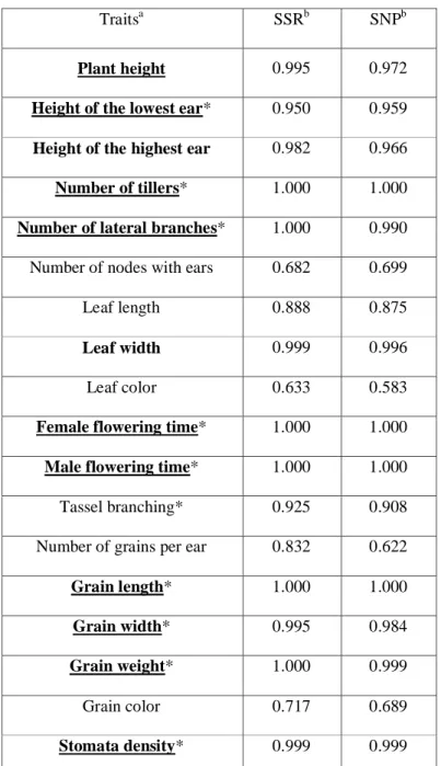
phenotypic differentiation under random genetic drift. Single-trait analyses revealed 283

evidence for spatially-varying selection at 12 traits, with high consistency between 284

SSRs and neutral SNPs (Table 1). Another method that contrasted genetic and 285

phenotypic differentiation (QST- FST) uncovered a large overlap with nine out of the 286

12 traits significantly deviating from the neutral model (Table 1) and one of the 287

remaining ones displaying borderline significance (Plant height=PL, S8 Fig). 288

Together, these two methods indicated that phenotypic divergence among populations 289

was driven by local selective forces. 290

Table 1. Signals of selection (posterior probability S) for each trait considering SSR markers (11 populations) or SNPs (10 populations).

Traitsa SSRb SNPb

Plant height 0.995 0.972

Height of the lowest ear* 0.950 0.959

Height of the highest ear 0.982 0.966

Number of tillers* 1.000 1.000

Number of lateral branches* 1.000 0.990 Number of nodes with ears 0.682 0.699

Leaf length 0.888 0.875

Leaf width 0.999 0.996

Leaf color 0.633 0.583

Female flowering time* 1.000 1.000

Male flowering time* 1.000 1.000

Tassel branching* 0.925 0.908 Number of grains per ear 0.832 0.622

Grain length* 1.000 1.000 Grain width* 0.995 0.984 Grain weight* 1.000 0.999 Grain color 0.717 0.689 Stomata density* 0.999 0.999 a

: Traits displaying signal of selection (spatially-varying traits, S > 0.95) are indicated in bold, and marked by an asterisk when significant in QST-FSTComp analysis. We considered the

b

: Values reported correspond to S from DRIFTSEL.S is the posterior probability that

divergence among populations was not driven by drift only. Following [60], we used here a conservative credibility value of S > 0.95 to declare divergent selection.

Altogether, evidence of spatially varying selection at 10 traits (Table 1) as

291

well as continuous variation of a subset of traits across populations in both elevation 292

gradients (Fig 2, S3 Fig) was consistent with a syndrome where populations produced 293

less tillers, flowered earlier, displayed lower stomata density and carried larger, 294

longer and heavier grains with increasing elevation. 295

296

Outlier detection and correlation with environmental variables.

297

We successfully genotyped 218 (~81%) out of 270 outlier SNPs on a broad set 298

of 28 populations, of which 141 were previously detected in candidate regions for 299

local adaptation [58].Candidate regions were originally identified from re-sequencing 300

data of only six teosinte populations (S1 Table) following an approach that included 301

high differentiation between highlands and lowlands, environmental correlation, and 302

in some cases their intersection with genomic regions involved in quantitative trait 303

variation in maize. The remaining outlier SNPs (77) were discovered in the present 304

study by performing FST-scans on the same re-sequencing data (S5 Table). We 305

selected outlier SNPs that were both highly differentiated between highland and 306

lowland populations within gradient (high/low in gradient a or b or both), and 307

between highland and lowland populations within subspecies in gradient b (high/low 308

within parviglumis, mexicana or both). FST-scans pinpointed three genomic regions of 309

particularly high differentiation (S9 Fig) that corresponded to previously described 310

inversions [55, 56]: one inversion on chromosome 1 (Inv1n), one on chromosome 4 311

(Inv4m) and one on the far end of chromosome 9 (Inv9e). 312

A substantial proportion of outlier SNPs was chosen based on their significant 313

correlation among six populations between variation of allele frequency and their 314

coordinate on the first environmental principal component [58]. We extended 315

environmental analyses to 171 outlier SNPs (MAF>5%) on a broader sample of 28 316

populations (S2 Fig) and used the two first components (PCenv1 and PCenv2) to 317

summarize environmental information. The first component, that explained 56% of 318

the variation, correlated with altitude but displayed no correlation to either latitude or 319

longitude. PCenv1 was defined both by temperature- and precipitation- related 320

variables (S2 B Fig) including Minimum Temperature of Coldest Month (T6), Mean 321

Temperature of Driest and Coldest Quarter (T9 and T11) and Precipitation of Driest 322

Month and Quarter (P14 and P17). The second PC explained 20.5% of the variation 323

and was mainly defined (S2 B Fig) by Isothermality (T3), Temperature Seasonality 324

(T4) and Temperature Annual Range (T7). 325

We first employed multiple regression to test for each SNP, whether the 326

pairwise FST matrix across 28 populations correlated to the environmental (distance 327

along PCenv1) and/or the geographical distance. As expected, we found a 328

significantly greater proportion of environmentally-correlated SNPs among outliers 329

compared with neutral SNPs (χ² =264.07, P-value=2.2 10-16), a pattern not seen with 330

geographically-correlated SNPs. That outlier SNPs displayed a greater isolation-by-331

environment than isolation-by-distance, indicated that patterns of allele frequency 332

differentiation among populations were primarily driven by adaptive processes. We 333

further tested correlations between allele frequencies and environmental variation. 334

Roughly 60.8% (104) of the 171 outlier SNPs associated with at least one of the two 335

first PCenvs, with 87 and 33 associated with PCenv1 and PCenv2, respectively, and 336

little overlap (S5 Table). As expected, the principal component driven by altitude 337

(PCenv1) correlated to allele frequency for a greater fraction of SNPs than the second 338

orthogonal component. Interestingly, we found enrichment of environmentally-339

associated SNPs within inversions both for PCenv1 (χ² = 14.63, P-value=1.30 10-4) 340

and PCenv2 (χ² = 33.77, P-value=6.22 10-9). 341

342

Associating genotypic variation to phenotypic variation.

343

We tested the association between phenotypes and 171 of the outlier SNPs 344

(MAF>5%) using the association panel. For each SNP-trait combination, the sample 345

size ranged from 264 to 1068, with a median of 1004 individuals (S6 Table). We used 346

SSRs to correct for both structure (at K=5) and kinship among individual genotypes. 347

This model (M5) resulted in a uniform distribution of P-values when testing the 348

association between genotypic variation at SSRs and phenotypic trait variation (S10 349

Fig). Under this model, we found that 126 outlier SNPs (73.7%) associated to at least 350

one trait (Fig 5 and S11 Fig) at an FDR of 10%. The number of associated SNPs per 351

trait varied from 0 for leaf and grain coloration, to 55 SNPs for grain length, with an 352

average of 22.6 SNPs per trait (S5 Table). Ninety-three (73.8%) out of the 126 353

associated SNPs were common to at least two traits, and the remaining 33 SNPs were 354

associated to a single trait (S5 Table). The ten traits displaying evidence of spatially 355

varying selection in the QST-FST analyses displayed more associated SNPs per trait 356

(30.5 on average), than the non-spatially varying traits (12.75 on average). 357

A growing body of literature stresses that incomplete control of population 358

stratification may lead to spurious associations [61]. Hence, highly differentiated 359

traits along environmental gradients are expected to co-vary with any variant whose 360

allele frequency is differentiated along the same gradients, without underlying causal 361

link. We therefore expected false positives in our setting where both phenotypic traits 362

and outlier SNPs varied with altitude. We indeed found a slightly significant 363

correlation (r=0.5, P-value=0.03) between the strength of the population effect for 364

each trait – a measure of trait differentiation (S3 Table) – and its number of associated 365

SNPs (S5 Table). 366

To verify that additional layers of structuring among populations did not cause 367

an excess of associations, we repeated the association analyzes considering a 368

structuring with 11 populations (instead of K=5) as covariate (M5’), a proxy of the 369

structuring revealed at K=11 (S6 Fig). With this level of structuring, we retrieved 370

much less associated SNPs (S5 Table). Among the 126 SNPs associating with at least 371

one trait at K=5, only 22 were recovered considering 11 populations. An additional 372

SNP was detected with structuring at 11 populations that was absent at K=5. Eight 373

traits displayed no association, and the remaining traits varied from a single 374

associated SNP (Leaf length – LeL and the number of tillers – Til) to 8 associated 375

SNPs for grain weight (S5 Table). For instance, traits such as female or male 376

flowering time that displayed 45 and 43 associated SNPs at K=5, now displayed only 377

4 and 3 associated SNPs, respectively (Fig 5). Note that one trait (Leaf color) 378

associated with 4 SNPs considering 11 populations while displaying no association at 379

K=5. Significant genetic associations were therefore highly contingent on the 380

population structure. Noteworthy, traits under spatially varying selection still 381

associated with more SNPs (2.00 on average) than those with no spatially varying 382

selection (1.25 SNPs on average). 383

384 385

Figure 5: Manhattan plots of associations between 171 outlier SNPs and 6

386

phenotypic traits. X-axis indicates the positions of outlier SNPs on chromosomes 1

387

to 10, black and gray colors alternating per chromosome. Plotted on the Y-axis are the 388

negative Log10-transformed P values obtained for the K=5 model. Significant

389

associations (10% FDR) are indicated considering either a structure matrix at K=5 390

(pink dots), 11 populations (blue dots) or both K=5 and 11 populations (purple dots) 391

models. 392

393

Altogether the 23 SNPs recovered considering a neutral genetic structure with 394

11 populations corresponded to 30 associations, 7 of the SNPs being associated to 395

more than one trait (S5 Table). For all these 30 associations except in two cases (FFT 396

with SNP_7, and MFT with SNP_28), the SNP effect did not vary among populations 397

(non-significant SNP-by-population interaction in model M5’ when we included the 398

SNP interactions with year*field and population). For a subset of two SNPs, we 399

illustrated the regression between the trait value and the shift of allele frequencies 400

with altitude (Fig 6 A&B). We estimated corresponding additive and dominance 401

effects (S7 Table). In some cases, the intra-population effect corroborated the inter-402

population variation with relatively large additive effects of the same sign (Fig 6 403

C&D). Note that in both examples shown in Fig 6, one or the other allele was 404

dominant. In other cases, the results were more difficult to interpret with negligible 405

additive effect but extremely strong dominance (S7 Table, SNP_210 for instance). 406

407 408 409

Figure 6: Regression of phenotypic average value on SNP allele frequency across

410

populations, and within-population average phenotypic value for each SNP

411

genotype. Per-population phenotypic average values of traits are regressed on alleles

412

frequencies at SNP_149 (A) and SNP_179 (B) with corresponding within-population 413

average phenotypic value per genotype (C & D). In A and B, the 11 populations of 414

the association panel are shown with parviglumis (green circles) and mexicana (red 415

triangles) populations sampled along gradient a and gradient b. Phenotypic average 416

values were corrected for the experimental design (calculated as the residues of model 417

M2). Pval refers to the P-value of the linear regression represented in blue. In C and 418

D, genotypic effects from model M5’ are expressed as the average phenotypic value 419

of heterozygotes (1) and homozygotes for the reference (0) and the alternative allele 420

(2). FDR values are obtained from the association analysis on 171 SNPs with 421

correction for genetic structure using 11 population. 422

423

Independence of SNPs associated to phenotypes.

424

We computed the pairwise linkage disequilibrium (LD) as measured by r2 425

between the 171 outlier SNPs using the R package LDcorSV [62]. Because we were 426

specifically interested by LD pattern between phenotypically-associated SNPs, as for 427

the association analyses we accounted for structure and kinship computed from SSRs 428

while estimating LD [63]. The 171 outlier SNPs were distributed along the 10 429

chromosomes of maize, and exhibited low level of linkage disequilibrium (LD), 430

except for SNPs located on chromosomes eight, nine, and a cluster of SNPs located 431

on chromosome 4 (S12 Fig). 432

Among the 171, the subset of 23 phenotypically-associated SNPs (detected 433

when considering the 11-population structure) displayed an excess of elevated LD 434

values – out of 47 pairs of SNPs phenotypically-associated to a same trait, 16 pairs 435

were contained in the 5% higher values of the LD distribution of all outlier SNP pairs. 436

Twelve out of the 16 pairs related to grain weight, the remaining four to leaf 437

coloration, and one pair of SNPs was associated to both traits. Noteworthy was that 438

inversions on chromosomes 1, 4, and 9, taken together, were enriched for 439

phenotypically-associated SNPs (χ² = 8.95, P-value=0.0028). We recovered a 440

borderline significant enrichment with the correction K=5 (χ² = 3.82, P-value=0.051). 441

Finally, we asked whether multiple SNPs contributed independently to the 442

phenotypic variation of a single trait. We tested a multiple SNP model where SNPs 443

were added incrementally when significantly associated (FDR < 0.10). We found 2, 3 444

and 2 SNPs for female, male flowering time and height of the highest ear, 445

respectively (S5 Table). Except for the latter trait, the SNPs were located on different 446 chromosomes. 447 448

Discussion

Plants are excellent systems to study local adaptation. First, owing to their 451

sessile nature, local adaptation of plant populations is pervasive [13]. Second, 452

environmental effects can be efficiently controlled in common garden experiments, 453

facilitating the identification of the physiological, morphological and phenological 454

traits influenced by spatially-variable selection [64]. Identification of the determinants 455

of complex trait variation and their covariation in natural populations is however 456

challenging [65]. While population genomics has brought a flurry of tools to detect 457

footprints of local adaptation, their reliability remains questioned [61]. In addition, 458

local adaptation and demographic history frequently follow the same geographic route, 459

making the disentangling of trait, molecular, and environmental variation, particularly 460

arduous. Here we investigated those links on a well-established outcrossing system, 461

the closest wild relatives of maize, along altitudinal gradients that display 462

considerable environmental shifts over short geographical scales. 463

464

The syndrome of altitudinal adaptation results from selection at multiple

co-465

adapted traits.

466

Common garden studies along elevation gradients have been conducted in 467

European and North American plants species [66]. Together with other studies, they 468

have revealed that adaptive responses to altitude are multifarious [67]. They include 469

physiological responses such as high photosynthetic rates [68], tolerance to frost [69], 470

biosynthesis of UV-induced phenolic components [70]; morphological responses with 471

reduced stature [71, 72], modification of leaf surface [73], increase in leaf non-472

glandular trichomes [74], modification of stomata density; and phenological 473

responses with variation in flowering time [75], and reduced growth period [76]. 474

Our multivariate analysis of teosinte phenotypic variation revealed a marked 475

differentiation between teosinte subspecies along an axis of variation (21.26% of the 476

total variation) that also discriminated populations by altitude (Fig 2A & B). The 477

combined effects of assortative mating and environmental elevation variation may 478

generate, in certain conditions, trait differentiation along gradients without underlying 479

divergent selection [77]. While we did not measure flowering time differences among 480

populations in situ, we did find evidence for long distance gene flow between 481

gradients and subspecies (Fig 4 A & C). In addition, several lines of arguments 482

suggest that the observed clinal patterns result from selection at independent traits and 483

is not solely driven by differences in flowering time among populations. First, two 484

distinct methods accounting for shared population history concur with signals of 485

spatially-varying selection at ten out of the 18 traits (Table 1). Nine of them exhibited 486

a clinal trend of increase/decrease of population phenotypic values with elevation (S3 487

Fig) within at least one of the two subspecies. This number is actually conservative, 488

because these approaches disregard the impact of selective constraints which in fact 489

tend to decrease inter-population differences in phenotypes. Second, while male and 490

female flowering times were positively correlated, they displayed only subtle 491

correlations (|r|<0.16) with other spatially-varying traits except for grain weight and 492

length (|r| <0.33). Third, we observed convergence at multiple phenotypes between 493

the lowland populations from the two gradients that occurred despite their 494

geographical and genetical distance (Fig 4) again arguing that local adaptation drives 495

the underlying patterns. 496

Spatially-varying traits that displayed altitudinal trends, collectively defined a 497

teosinte altitudinal syndrome of adaptation characterized by early-flowering, 498

production of few tillers albeit numerous lateral branches, production of heavy, long 499

and large grains, and decrease in stomata density. We also observed increased leaf 500

pigmentation with elevation, although with a less significant signal (S3 Table), 501

consistent with the pronounced difference in sheath color reported between 502

parviglumis and mexicana [78, 79]. Because seeds were collected from wild 503

populations, a potential limitation of our experimental setting is the confusion 504

between genetic and environmental maternal effects. Environmental maternal effects 505

could bias upward our heritability estimates. However, our results corroborate 506

previous findings of reduced number of tillers and increased grain weight in mexicana 507

compared with parviglumis [80]. Thus although maternal effects could not be fully 508

discarded, we believe they were likely to be weak. 509

The trend towards depleted stomata density at high altitudes (S3 Fig) could 510

arguably represent a physiological adaptation as stomata influence components of 511

plant fitness through their control of transpiration and photosynthetic rate [81]. Indeed, 512

in natural accessions of A. thaliana, stomatal traits showed signatures of local 513

adaptation and were associated with both climatic conditions and water-use efficiency 514

[82]. Furthermore, previous work has shown that in arid and hot highland 515

environments, densely-packed stomata may promote increased leaf cooling in 516

response to desiccation [83] and may also counteract limited photosynthetic rate with 517

decreasing pCO2 [84]. Accordingly, increased stomata density at high elevation sites

518

has been reported in alpine species such as the European beech [85] as well as in 519

populations of Mimulus guttatus subjected to higher precipitations in the Sierra 520

Nevada [86]. In our case, higher elevations display both arid environment and cooler 521

temperatures during the growing season, features perhaps more comparable to other 522

tropical mountains for which a diversity of patterns in stomatal density variation with 523

altitude has been reported [87]. Further work will be needed to decipher the 524

mechanisms driving the pattern of declining stomata density with altitude in teosintes. 525

Altogether, the altitudinal syndrome was consistent with natural selection for rapid 526

life-cycle shift, with early-flowering in the shorter growing season of the highlands 527

and production of larger propagules than in the lowlands. This altitudinal syndrome 528

evolved in spite of detectable gene flow. 529

Although we did not formally measure biomass production, the lower number 530

of tillers and higher amount and size of grains in the highlands when compared with 531

the lowlands may reflect trade-offs between allocation to grain production and 532

vegetative growth [88]. Because grains fell at maturity and a single teosinte individual 533

produces hundreds of ears, we were unable to provide a proxy for total grain 534

production. The existence of fitness-related trade-offs therefore still needs to be 535

formally addressed. 536

Beyond trade-offs, our results more generally question the extent of 537

correlations between traits. In maize, for instance, we know that female and male 538

flowering time are positively correlated and that their genetic control is in part 539

determined by a common set of genes [89]. They themselves further increase with 540

yield-related traits [90]. Response to selection for late-flowering also led to a 541

correlated increase in leaf number in cultivated maize [91], and common genetic loci 542

have been shown to determine these traits as well [92]. Here we found strong positive 543

correlations between traits: male and female flowering time, grain length and width, 544

plant height and height of the lowest or highest ear. Strong negative correlations were 545

observed instead between grain weight and both male and female flowering time. 546

Trait correlations were therefore partly consistent with previous observations in maize, 547

suggesting that they were inherited from wild ancestors. 548

549

Footprints of past adaptation are relevant to detect variants involved in present

550

phenotypic variation.

551

The overall level of differentiation in our outcrossing system (FST ≈22%) fell 552

within the range of previous estimates (23% [93]and 33% [55] for samples 553

encompassing both teosinte subspecies). It is relatively low compared to other 554

systems such as the selfer Arabidopsis thaliana, where association panels typically 555

display maximum values of FST around 60% within 10kb-windows genome-wide [94]. 556

Nevertheless, correction for sample structure is key for statistical associations 557

between genotypes and phenotypes along environmental gradients. This is because 558

outliers that display lowland/highland differentiation co-vary with environmental 559

factors, which themselves may affect traits [95]. Consistently, we found that 73.7% 560

SNPs associated with phenotypic variation at K=5, but only 13.5% of them did so 561

when considering a genetic structure with 11 populations. Except for one, the latter 562

set of SNPs represented a subset of the former. Because teosinte subspecies 563

differentiation was fully accounted for at K=5 (as shown by the clear distinction 564

between mexicana populations and the rest of the samples, Fig 4A), the inflation of 565

significant associations at K=5 is not due to subspecies differentiation, but rather to 566

residual stratification among populations within genetic groups. Likewise, recent 567

studies in humans, where global differentiation is comparatively low [96] have shown 568

that incomplete control for population structure within European samples strongly 569

impacts association results [61, 97]. Controlling for such structure may be even more 570

critical in domesticated plants, where genetic structure is inferred a posteriori from 571

genetic data (rather than a priori from population information) and pedigrees are 572

often not well described. Below, we show that considering more than one correction 573

using minor peaks delivered by the Evanno statistic (S5 Fig) can be informative. 574

Considering a structure with 5 genetic groups, the number of SNPs associated 575

per trait varied from 1 to 55, with no association for leaf and grain coloration (S5 576

Table). False positives likely represent a greater proportion of associations at K=5 as 577

illustrated by a slight excess of small P-values when compared with a correction with 578

11 populations for most traits (S10 Fig). Nevertheless, our analysis recovered credible 579

candidate adaptive loci that were no longer associated when a finer-grained 580

population structure was included in the model. For instance at K=5, we detected 581

Sugary1 (Su1), a gene encoding a starch debranching enzyme that was selected during 582

maize domestication and subsequent breeding [98, 99]. We found that Su1 was 583

associated with variation at six traits (male and female flowering time, tassel 584

branching, height of the highest ear, grain weight and stomata density) pointing to 585

high pleiotropy. A previous study reported association of this gene to oil content in 586

teosintes [100]. In maize, this gene has a demonstrated role in kernel phenotypic 587

differences between maize genetic groups [101]. Su1 is therefore most probably a 588

true-positive. That this gene was no longer recovered with the 11-population structure 589

correction indicated that divergent selection acted among populations. Indeed, allelic 590

frequency was highly contrasted among populations, with most populations fixed for 591

one or the other allele, and a single population with intermediate allelic frequency. 592

With the 11-population correction, very low power is thus left to detect the effect of 593

Su1 on phenotypes. 594

Although the confounding population structure likely influenced the genetic 595

associations, experimental evidence indicates that an appreciable proportion of the 596

variants recovered with both K=5 and 11 populations are true-positives (S5 Table). 597

One SNP associated with female and male flowering time, as well as with plant height 598

and grain length (at K=5 only for the two latter traits) maps within the phytochrome 599

B2 (SNP_210; phyB2) gene. Phytochromes are involved in perceiving light signals 600

and are essential for growth and development in plants. The maize gene phyB2 601

regulates the photoperiod-dependent floral transition, with mutants producing early 602

flowering phenotypes and reduced plant height [102]. Genes from the 603

phosphatidylethanolamine-binding proteins (PEBPs) family – Zea mays 604

CENTRORADIALIS (ZCN) family in maize – are also well-known to act as promotor 605

and repressor of the floral transition in plants [103]. ZCN8 is the main floral activator 606

of maize [104], and both ZCN8 and ZCN5 strongly associate with flowering time 607

variation [101, 105]. Consistently, we found associations of male and female 608

flowering time with PEBP18 (SNP_15). It is interesting to note that SNPs at two 609

flowering time genes, phyB2 and PEBP18, influenced independently as well as in 610

combination both female and male flowering time variation (S5 Table). 611

The proportion of genic SNPs associated to phenotypic variation was not 612

significantly higher than that of non-genic SNPs (i.e, SNPs >1kb from a gene) (χ²(df=1)

613

= 0.043, P-value = 0.84 at K=5 and χ²(df=1) =1.623, P-value =0.020 with 11

614

populations) stressing the importance of considering both types of variants [106]. For 615

instance, we discovered a non-genic SNP (SNP_149) that displayed a strong 616

association with leaf width variation as well as a pattern of allele frequency shift with 617

altitude among populations (Fig 6B). 618

619

Physically-linked and independent SNPs both contribute to the establishment of

620

adaptive genetic correlations.

621

We found limited LD among our outlier SNPs (S10 Fig) corroborating 622

previous reports (LD decay within <100bp, [58, 93]). However, the subset of 623

phenotypically-associated SNPs displayed greater LD, a pattern likely exacerbated by 624

three Mb-scale inversions located on chromosomes 1 (Inv1n), 4 (Inv4m) and 9 (Inv9e) 625

that, taken together, were enriched for SNPs associated with environmental variables 626

related to altitude and/or SNPs associated with phenotypic variation. Previous work 627

[55, 56] has shown that Inv1n and Inv4m segregate within both parviglumis and 628

mexicana, while two inversions on chromosome 9, Inv9d and Inv9e, are present only 629

in some of the highest mexicana populations; such that all four inversions also follow 630

an altitudinal pattern. Our findings confirmed that three of these inversions possessed 631

an excess of SNPs with high FST between subspecies and between low- and high-632

mexicana populations for Inv9e [57]. Noteworthy Inv9d contains a large ear leaf 633

width quantitative trait locus in maize [106]. Corroborating these results, we found 634

consistent association between the only SNP located within this inversion and leaf 635

width variation in teosinte populations (S5 Table). Overall, our results further 636

strengthen the role of chromosomal inversions in teosinte altitudinal adaptation. 637

Because inversions suppress recombination between inverted and non-inverted 638

genotypes, their spread has likely contributed to the emergence and maintenance of 639

locally adaptive allelic combinations in the face of gene flow, as reported in a 640

growing number of other models (reviewed in [107]) including insects [108], fish 641

[109], birds [110] and plants [26, 111]. But we also found three cases of multi-SNP 642

determinism of traits (male and female flowering time and height of the highest ear, 643

Table S5) supporting selection of genetically independent loci. Consistently with 644

Weber et al. [100], we found that individual SNPs account for small proportions of 645

the phenotypic variance (S7 Table). Altogether, these observations are consistent with 646

joint selection of complex traits determined by several alleles of small effects, some 647

of which being maintained in linkage through selection of chromosomal 648 rearrangements. 649 650 Conclusion. 651 652

Elevation gradients provide an exceptional opportunity for investigating 653

variation of functional traits in response to continuous environmental factors at short 654

geographical scales. Here we documented patterns indicating that local adaptation, 655

likely facilitated by the existence of chromosomal inversions, allows teosintes to cope 656

with specific environmental conditions in spite of gene flow. We detected an 657

altitudinal syndrome in teosintes composed of sets of independent traits evolving 658

under spatially-varying selection. Because traits co-varied with environmental 659

differences along gradients, however, statistical associations between genotypes and 660

phenotypes largely depended on control of population stratification. Yet, several of 661

the variants we uncovered seem to underlie adaptive trait variation in teosintes. 662

Adaptive teosinte trait variation is likely relevant for maize evolution and breeding. 663

Whether the underlying SNPs detected in teosintes bear similar effects in maize or 664

whether their effects differ in domesticated backgrounds will have to be further 665

investigated. 666

Material and Methods

667 668

Description of teosinte populations and sampling.

669

We used 37 teosinte populations of mexicana (16) and parviglumis (21) 670

subspecies from two previous collections [57, 58, 112] to design our sampling. These 671

populations (S1 Table) are distributed along two altitudinal gradients (Fig 1). We 672

plotted their altitudinal profiles using R ‘raster’ package [113] (S1 Fig). We further 673

obtained 19 environmental variable layers from 674

http://idrisi.uaemex.mx/distribucion/superficies-climaticas-para-mexico. These high-675

resolution layers comprised monthly values from 1910 to 2009 estimated via 676

interpolation methods [107]. We extracted values of the 19 climatic variables for each 677

population (S1 Table). Note that high throughput sequencing (HTS) data were 678

obtained in a previous study for six populations out of the 37 (M6a, P1a, M7b, P2b, 679

M1b and P8b; Fig 1, S1 Table) to detect candidate genomic regions for local 680

adaptation [58]. The four highest and lowest of these populations were included in the 681

association panel described below. 682

We defined an association panel of 11 populations on which to perform a 683

genotype-phenotype association study (S1 Table). Our choice was guided by grain 684

availability as well as the coverage of the whole climatic and altitudinal ranges. 685

Hence, we computed Principal Component Analyses (PCA) for each gradient from 686

environmental variables using the FactoMineR package in R [114] and added altitude 687

to the PCA graphs as a supplementary variable. Our association panel comprised five 688

populations from a first gradient (a) – two mexicana and three parviglumis, and six 689

populations from a second gradient (b) – one mexicana and five parviglumis (Fig 1). 690

Finally, we extracted available SNP genotypes generated with the 691

MaizeSNP50 Genotyping BeadChip for 28 populations out of our 37 populations [57] 692

(S1 Table). From this available SNP dataset, we randomly sampled 1000 SNPs found 693

to display no selection footprint [57], hereafter neutral SNPs. Data for neutral SNPs 694

(Data S1) are available at: 10.6084/m9.figshare.9901472. We used this panel of 28 695

populations to investigate correlation with environmental variation. Note that 10 out 696

of the 28 populations were common to our association panel, and genotypes were 697

available for 24 to 34 individuals per population, albeit different from the ones of our 698

association mapping panel. 699

Common garden experiments

700

We used two common gardens for phenotypic evaluation of the association 701

panel (11 populations). Common gardens were located at INIFAP (Instituto Nacional 702

de Investigaciones Forestales, Agricolas y Pecuaria) experimental field stations in the 703

state of Guanajuato in Mexico, one in Celaya municipality at the Campo 704

Experimental Bajío (CEBAJ) (20°31’20’’ N, 100°48’44’’W) at 1750 meters of 705

elevation, and one in San Luis de la Paz municipality at the Sitio Experimental Norte 706

de Guanajuato (SENGUA) (21°17’55’’N, 100°30’59’’W) at 2017 meters of elevation. 707

These locations were selected because they present intermediate altitudes (S1 Fig). 708

The two common gardens were replicated in 2013 and 2014. 709

The original sampling contained 15 to 22 mother plants per population. Eight 710

to 12 grains per mother plant were sown each year in individual pots. After one 711

month, seedlings were transplanted in the field. Each of the four fields (2 locations, 2 712

years) was separated into four blocks encompassing 10 rows and 20 columns. We 713

evaluated one offspring of ~15 mother plants from each of the 11 teosinte populations 714

in each block, using a semi-randomized design, i.e. each row containing one or two 715

individuals from each population, and individuals being randomized within row, 716

leading to a total of 2,640 individual teosinte plants evaluated. 717

718

SSR genotyping and genetic structuring analyses on the association panel

719

In order to quantify the population structure and individual kinship in our 720

association panel, we genotyped 46 SSRs (S4 Table). Primers sequences are available 721

from the maize database project [115] and genotyping protocol were previously 722

published [116]. Genotyping was done at the GENTYANE platform (UMR INRA 723

1095, Clermont-Ferrand, France). Allele calling was performed on electropherograms 724

with the GeneMapper® Software Applied Biosystems®. Allele binning was carried 725

out using Autobin software [117], and further checked manually. 726

We employed STRUCTURE Bayesian classification software to compute a 727

genetic structure matrix on individual genotypes. Individuals with over 40% missing 728

data were excluded from analysis. For each number of clusters (K from 2 to 13), we 729

performed 10 independent runs of 500,000 iterations after a burn-in period of 50,000 730

iterations, and combined these 10 replicates using the LargeKGreedy algorithm from 731

the CLUMPP program [118]. We plotted the resulting clusters using DISTRUCT 732

software. We then used the Evanno method [119] to choose the optimal K value. We 733

followed the same methodology to compute a structure matrix from the outlier SNPs. 734

We inferred a kinship matrix K from the same SSRs using SPAGeDI [120]. 735

Kinship coefficients were calculated for each pair of individuals as correlation 736

between allelic states [121]. Since teosintes are outcrossers and expected to exhibit an 737

elevated level of heterozygosity, we estimated intra-individual kinship to fill in the 738

diagonal. We calculated ten kinship matrices, each excluding the SSRs from one out 739

of the 10 chromosomes. Microsatellite data (Data S2) are available 740

at: 10.6084/m9.figshare.9901472 741

In order to gain insights into population history of divergence and admixture, 742

we used 1000 neutral SNPs (i.e. SNPs genotyped by Aguirre-Liguori and 743

collaborators [57] and that displayed patterns consistent with neutrality among 49 744

teosinte populations) genotyped on 10 out of the 11 populations of the association 745

panel to run a TreeMix analysis (TreeMix version 1.13 [122]. TreeMix models 746

genetic drift to infer populations splits from an outgroup as well as migration edges 747

along a bifurcating tree. We oriented the SNPs using the previously published 748

MaizeSNP50 Genotyping BeadChip data from the outgroup species Tripsacum 749

dactyloides [55]. We tested from 0 to 10 migration edges. We fitted both a simple 750

exponential and a non-linear least square model (threshold of 1%) to select the 751

optimal number of migration edges as implemented in the OptM R package [123]. We 752

further verified that the proportion of variance did not substantially increase beyond 753

the optimal selected value. 754

755

Phenotypic trait measurements

756

We evaluated a total of 18 phenotypic traits on the association panel (S2 757

Table). We measured six traits related to plant architecture (PL: Plant Height, HLE: 758

Height of the Lowest Ear, HHE: Height of the Highest Ear, Til: number of Tillers, 759

LBr: number of Lateral Branches, NoE: number of Nodes with Ears), three traits 760

related to leave morphologies (LeL: Leaf Length, LeW: Leaf Width, LeC: Leaf 761

Color), three traits related to reproduction (MFT: Male Flowering Time, FFT: Female 762

Flowering Time, TBr : Tassel Branching), five traits related to grains (Gr: number of 763

Grains per ear, GrL: Grain Length, GrWi: Grain Width, GrWe: Grain Weight, GrC: 764

Grain Color), and one trait related to Stomata (StD: Stomata Density). These traits 765

were chosen because we suspected they could contribute to differences among 766

teosinte populations based on a previous report of morphological characterization on 767

112 teosinte collections grown in five localities [124]. 768

We measured the traits related to plant architecture and leaves after silk 769

emergence. Grain traits were measured at maturity. Leaf and grain coloration were 770

evaluated on a qualitative scale. For stomata density, we sampled three leaves per 771

plant and conserved them in humid paper in plastic bags. Analyses were undertaken at 772

the Institute for Evolution and Biodiversity (University of Münster) as followed: 5mm 773

blade discs were cut out from the mid length of one of the leaves and microscopic 774

images were taken after excitation with a 488nm laser. Nine locations (0.15mm2) per 775

disc were captured with 10 images per location along the z-axis (vertically along the 776

tissue). We automatically filtered images based on quality and estimated leaf stomata 777

density using custom image analysis algorithms implemented in Matlab. For each 778

sample, we calculated the median stomata density over the (up to) nine locations. To 779

verify detection accuracy, manual counts were undertaken for 54 random samples. 780

Automatic and manual counts were highly correlated (R²=0.82), indicating reliable 781

detection (see S1 Annex StomataDetection, Dittberner and de Meaux, for a detailed 782

description). The filtered data set of phenotypic measurements (Data S3) is available 783

at: 10.6084/m9.figshare.9901472. 784

785

Statistical analyses of phenotypic variation

786

In order to test for genetic effects on teosinte phenotypic variation, we 787

decomposed phenotypic values of each trait considering a fixed population effect plus 788

a random mother-plant effect (model M1): 789