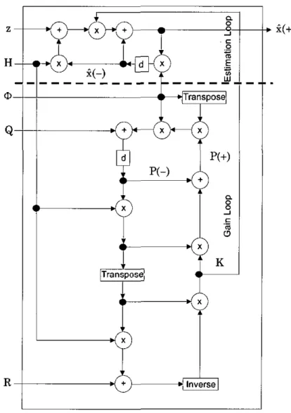
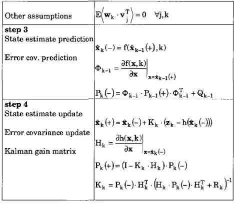
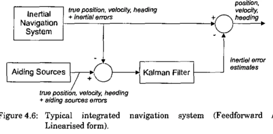
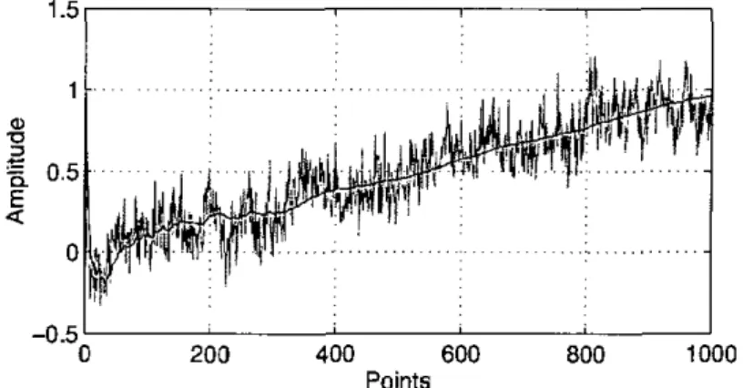
Data processing of a navigation microsystem
Texte intégral
Figure
Documents relatifs
Compared with the native French population, immigrants’ health status has deteriorated over the last thirty years and disparities seem to be more important among first
This problem can be solved by Blockchain based solutions where Individual can develop the sovereign controller of their own identity credentials.. Our objective is to develop
We can prove a similar Carleman estimate where the right-hand side is estimated in an H −1 -weighted space (Imanuvilov and.. In particular, in [12,26,30], determination problems
With this work, we demonstrate SALUS Patient History Tool which presents patient summaries to the clinical researcher by retrieving the values of the patient data fields from
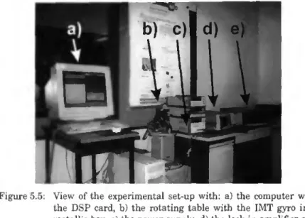
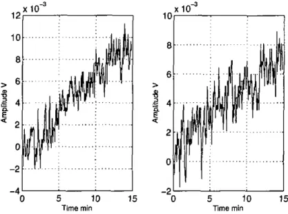
In this paper, the design of a three axis navigation microsystem was presented in four parts : the accelerometer, the angular rate sensor, simulation, and data processing. The
Ce but est atteint selon la presente invention grace a un detecteur de pression caracterise par le fait que la jante de la roue est realisee en un materiau amagnetique, le capteur
Le nouveau produit comporte de la sphaigne blanchie en combinaison avec de la pulpe de bois mecanique flnement dlvisee ayant one valeur CSF (Canadian Standart Freeness est
The process that led the University of Foggia to define the guidelines behind the design of the online courses available on the EduOpen platform is illustrated below, including
