Atmospheric Temperature Profile Retrievals Using
54
and
118-GHz Spectral Observations from the Proteus Aircraft
by
Andrew Sanchez
B.S.E., Arizona State University (1999)
Submitted to the Department of Electrical Engineering and Computer Science in partial
fulfillment of the requirements for the degree of
Master of Science
at the
MASSACHUSETTS INSTITUTE OF TECHNOLOGY
February 2002
© Massachusetts Institute of Technology 2002. All rights reserved.
A uthor... ... ...
Department of Electrical Engineering and Computer Science
February 10, 2003
Certified by...
.
David H. Staelin
Professor of Electrical Engineering
.-Vhesjs
SupervisorAccepted by...
Chairman, Departmental Committee
OF TECHNOLOGY
Arthur C. Smith
on Graduate Students
Atmospheric Temperature Profile Retrievals Using
54
and
118-GHz Spectral Observations from the Proteus Aircraft
by
Andrew Sanchez
Submitted to the Department of Electrical Engineering and Computer Science On February, 03, 2002 in partial fulfillment of the
requirements for the degree of
Master of Science in Electrical Engineering and Computer Science
Abstract
Temperature profile retrievals based on passive microwave spectral observations from an aircraft were made with a Linear Least Squares Estimator (LLSE). The National Polar-orbiting Observational Environmental Satellite System (NPOESS) Aircraft Satellite Testbed-Microwave (NAST-M) is an imaging passive spectrometer observing oxygen absorption bands at 50-57 GHz and 118.75 ± 0.8 - 118.75 ± 3.5 GHz.
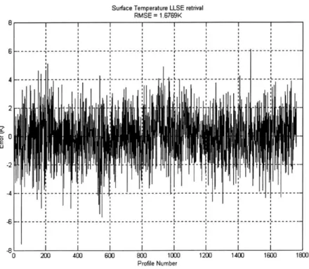
NAST-M can accurately measure brightness temperatures aboard Scaled Composite's Proteus Aircraft from an altitude of 16 km. Simulating the brightness temperatures NAST-M would observe required the use of the TIGR profile set of 1761 radiosondes from around the world. Using the entire set of simulated data, the RMS retrieval error averaged <2K for pressure levels from the surface to the aircraft.
Data collected for retrievals were measured during CLOUDIOP, WVIOP, and AFWEX deployments over the Southern Great Plains. The flights occurred during March 2000, October 2000, and December 2000 respectively. Six flights have been studied for naturally occurring phenomenon. Using radiosondes collected from the Atmospheric Radiation Measurement (ARM) Program, a gain and baseline calibration correction was implemented to improve the accuracy of temperature profile retrievals for a particular day. Sensitivity of the NAST-M data was approximately ± 0.5K and ± 0.8K for 54 and 118-GHz spectrometers respectively, with the exception of channel 1 for both systems. Additive RMS noise due to calibration drift, interference, or unknown causes was calculated to be -0.1K and -0.5K respectively.
Thesis Supervisor: David H. Staelin Title: Professor of Electrical Engineering
Acknowledgements
I would like to start out by giving much thanks to my wife Roni D. She has stood
by my side through life's hardships ever since we met in 1995. I want to thank her for
taking good care of our family and me while living at MIT. I want to thank my son
Gabriel for always making me smile through his learning experiences. I want to thank
my twins Adrianna and Alexander for making me realize that we can survive through
anything. I want to thank my mom for always helping out when I was in financial
turmoil. Helping us transplant across the country was a big help. Also I will never forget
how you always push me to keep going when I decide to procrastinate at times. Thanks
mom! I also want to thank my wife's parents, Ron and Brenda Johnson, for advice in
life. You make me see that situations are really better then they appear. I want to thank
my little bro, Frank, for helping me move out of the apartment this summer. Same goes
for you too Jose and also for pointing out that I am such a pack rat. I want to thank my
Dad, my Uncle Sang Sop, Larry, and my Halmoni for always being there. Thanks.
I want to thank Prof. David H. Staelin for his guidance, support, and patience
throughout the course of this research. He has been a very important resource for
completing this thesis. Thank you. I appreciate the opportunity of upgrading NAST-M.
I want to give thanks to Phil Rosenkranz for answering my questions regarding
atmospheric modeling. I want to thank R. Vincent Leslie, Fred W. Chen, and Bill
Blackwell for helping me with my questions on NAST-M and MATLAB. I want to
thank Chuck Cho for my Linux support. I would like to thank Amy Mueller for chatting
with me once in a while and helping me with MATLAB. I would like to thank Dave
Foss and Maxine Samuels of RLE for helping me with software and for ordering
numerous circuit components for me. Finally, I give thanks to Marilyn Pierce for her
suggestions and support. She has helped me in so many ways and has made my stay at
MIT an experience I will never forget.
This research has been funded by the National Consortium for Graduate Degrees
for Minorities in Engineering and Science, Inc., the Department of Electrical Engineering
and Computer Science, MIT, and the Research Laboratory of Electronics, MIT.
Contents
Chapter 1...
15
1 Introduction ...
15
1.1 M otivation ...
15
1.2 Thesis Outline ...
15
Chapter 2...
18
2 Fundam entals of Rem ote Sensing ... 18
2.1 Physics...
18
2.1.1 Radiative Transfer Equation... 19
2.2 M athem atics ... 21
2.2.1 Bayes' Least-Squares Estim ation... 22
2.2.2 Linear Least-Squares Estim ator ... 22
2.2.3 Linear Regression... 24
Chapter 3...27
3 D ata ... 27
3.1 N A ST-M Instrum ent Overview ... 27
3.1.1 Calibration... 29
3.1.2 Correction for therm al gradients in the hot load ... 30
3.1.3 A ntenna beam spillover correction ... 31
3.1.4 Instrum ent Sensitivity ... 31
3.1.5 Brightness Tem perature Post Processing ... 32
3.2 TIG R profile set ... 32
3.2.1 Simulating Brightness Temperature Components ... 33
3.3 A tm ospheric Radiation M easurem ent Program ... 33
3.3.1 Partial atm osphere vs. Entire Atm osphere ... 34
3.3.2 Simulation of Brightness Temperatures from ARM... 35
3.4 CLOUDIOP, WVIOP, and AFWEX Deployments ... 36
3.5 Bias rem oval... 36
3.5.1 Calculated G ain and Baseline ... 41
Chapter 4... 45
4 Retrieval A lgorithm ... 45
4.1 Overview of the A lgorithm ... 45
4. 1.1 LLSE Retrieval Algorithm ... 45
4.1.2 Finding an LLSE ... 46
4.1.3 Results ... 47
Chapter 5... 53
5 NAST-M CLOUDIOP, WVIOP, and AFWEX Retrievals ... 53
5.1 CLOU D IOP Retrievals ... 53
5.1.1 CLOU D IOP Retrieval Results ... 54
5.2 W V IOP Retrievals...
59
5.2.1 W V IOP Retrieval Results ... 60
5.3 AFW EX Retrievals ... 65
5.3.1 A FW EX Retrieval Results ...
66
6 Conclusions and Future Work...73
6.1 Future W ork ...
74
Appendix A: Select MATLAB Code ...
76
A. 1 NAST-M Calibration Routine with Spillover Correction...76
A.2 Routine for Interpolating NAST-M Scan Times to GPS Time...78
A.3 Quicklook Chart Generation Script...81
Appendix B : LLSE Preparation and Development ...
87
B.1 TIGR Data Set Reader...
87
B.2 Calculation of Brightness Temperature Components...
89
B.3 ARM Brightness Temperature Components Simulation...91
B.4 NAST-M Brightness Temperature Simulation...94
B.5 LLSE Development ...
96
B.6 Temperature Retrieval Code...
99
A ppendix C : M ore Im ages ...
108
C. 1 Additional Imagery from CLOUDIOP...
108
C.2 Additional Imagery from WVIOP...
126
C.3 Additional Imagery from AFWEX...
142
List of Figures
Figure 2-1 Geometric Layout for a Planar Stratified Atmosphere...
20
Figure 3-1 Different Configurations of the Proteus. ...
29
Figure 3-2 Southern Great Plains and Radiosonde Sites...
34
Figure 3-3 Partial Atmosphere vs. Full Atmosphere...
35
Figure 3-4 Example of Gain and Baseline Correction... 37
Figure 3-5 Example of Brightness Temperature Correction... 38
Figure 3-6 Measured 54-GHz data over all spots. ... 39
Figure 3-7 Simulated 54-GHz data over all spots... 40
Figure 3-8 Measured 118-GHz data over all spots. ... 40
Figure 3-9 Simulated 118-GHz data over all spots... 41
Figure 3-10 Brightness Temperature Difference over all spots...41
Figure 4-1 Super Set of Simulated TIGR Brightness Temperatures... 46
Figure 4-2 RMS Retrieval Error of the TIGR Ensemble. ... 48
Figure 4-3 RMS Retrieval Error of the ARM Ensemble. ... 48
Figure 4-4 Surface Temperature Retrieval Error on TIGR ... 49
Figure 4-5 Surface Temperature Retrieval Error on ARM. ... 49
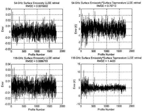
Figure 4-6 Surface Emissivity and Product of Surface Emissivity with Surface Temperature Retrieval Error on TIGR. ... 50
Figure 4-7 Surface Emissivity and Product of Surface Emissivity with Surface Temperature Retrieval Error on ARM . ... 50
Figure 4-8 RMS Error of Closed Loop Test on TIGR ... 51
Figure 4-9 RMS Error of Closed Loop Test on ARM. ... 51
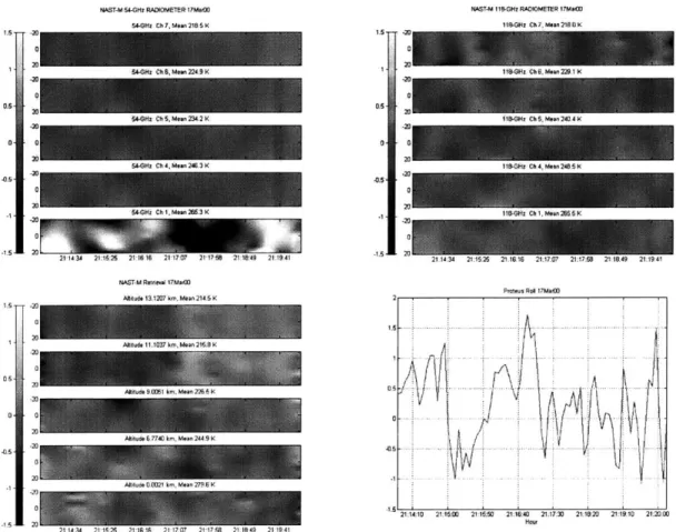
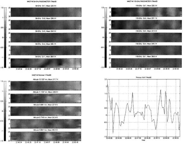
Figure 5-1 17M arOO Flight Path... 54
Figure 5-2 17MarOO Temperature Retrieval Comparison for index 1300. ... 54
Figure 5-3 17MarOO Temperature Imagery Comparison for index 1300...55
Figure 5-4 17MarOO Temperature Retrieval Comparison for Index 2370...55
Figure 5-5 17MarOO Temperature Imagery for index 2370. ... 56
Figure 5-6 l9M arOO Flight Path... 57
Figure 5-7 l9MarOO Temperature Retrieval Comparison for index 1620. ... 57
Figure 5-8 l9MarOO Temperature Imagery for index 1620. ... 58
Figure 5-9 l9MarOO Temperature Comparison for index 2915... 58
Figure 5-10 l9MarOO Temperature Imagery for index 2915...59
Figure 5-11 040ctOO Flight Path...
60
Figure 5-12 04OctOO Temperature Retrieval Comparison for index 1600. ... 60
Figure 5-13 04OctOO Temperature Imagery for index 1600...61
Figure 5-14 04OctOO Temperature Retrieval Comparison for index 2795. ... 61
Figure 5-15 040ctOO Temperature Imagery for index 2795...62
Figure 5-16 06OctOO Flight Path...
63
Figure 5-17 06OctOO Temperature Retrieval Comparison for index 1110. ... 63
Figure 5-18 060ctOO Temperature Imagery for index 1110...64
Figure 5-19 060ctOO Temperature Retrieval Comparison for index 1608. ... 64
Figure 5-20 060ctOO Temperature Imagery for index 1608...65
03DecOO Temperature Retrieval Comparison for index 841. ...
66
03Dec00Temperature Imagery for index 841. ...
67
03Dec00Temperature Retrieval Comparison for index 1009. ...
67
03Dec00Temperature Imagery for index 1009. ...
68
06D ecOO Flight Path...
69
06DecOO Temperature Retrieval Comparison for index 1561. ...
69
06DecOO Temperature Imagery for index 1561. ...
70
06DecOO Temperature Retrieval Comparison for index 1777. ...
70
06DecOO Temperature Imagery for index 1777. ...
71
Figure
Figure
Figure
Figure
Figure
Figure
Figure
Figure
Figure
Figure
Figure
Figure
Figure
Figure
Figure
Figure
Figure
Figure
Figure
Figure
Figure
Figure
Figure
Figure
Figure
Figure
Figure
Figure
Figure
Figure
Figure
Figure
Figure
Figure
Figure
Figure
Figure
Figure
Figure
Figure
Figure
Figure
Figure
Figure
Figure
5-22
5-23
5-24
5-25
5-26
5-27
5-28
5-29
5-30
C-1 I
C-2 1
C-3 1
C-4 1
C-5 I
C-6 1
C-7 1
C-8 1
C-9 1
C-10
C-1
C-12
C-13
C-14
C-15
C-16
C-17
C-18
C-19
C-20
C-21
C-22
C-23
C-24
C-25
C-26
C-27
C-28
C-29
C-30
C-31
C-32
C-33
C-34
C-35
C-36
Retrieval Comparison for index 1400...
Imagery for index 1400. ...
Retrieval Comparison for index 1900...
Imagery for index 1900. ...
Retrieval Comparison for index 2020...
Imagery for index 2020. ...
Retrieval Comparison for index 2195...
Imagery for index 2195. ...
Retrieval Comparison for index 1110...
108
109
109
109
110
110
111
111
112
Figure C-37 04OctOO Temperature Retrieval Comparison for index 1060. ... 126
7MarOO Temperature
7MarOO Temperature
7MarOO Temperature
7MarOO Temperature
7MarOO Temperature
7MarOO Temperature
7MarOO Temperature
7MarOO Temperature
9MarOO Temperature
Temperature
Temperature
Temperature
Temperature
Temperature
Temperature
Temperature
Temperature
Temperature
Temperature
Temperature
Temperature
Temperature
Temperature
Temperature
Temperature
Temperature
Temperature
Temperature
Temperature
Temperature
Temperature
Temperature
Temperature
Temperature
Temperature
Temperature
l9MarOO
l9MarOO
l9MarOO
l9MarOO
19MarOO
l9MarOO
19MarOO
19MarOO
l9MarOO
19MarOO
l9MarOO
19MarOO
19MarOO
19MarOO
19MarOO
19MarOO
l9MarOO
l9MarOO
19MarOO
19MarOO
19MarOO
19MarOO
19MarOO
19MarOO
19MarOO
l9MarOO
19MarOO
Imagery for index 1110. ...
112
Retrieval Comparison for index 1260... 113
Imagery for index 1260. ...
113
Retrieval Comparison for index 1400... 114
Imagery for index 1400. ...
114
Retrieval Comparison for index 1460... 115
Imagery for index 1460. ...
115
Retrieval Comparison for index 1550... 116
Imagery for index 1550 ...
116
Retrieval Comparison for index 1735... 117
Imagery for index 1735. ...
117
Retrieval Comparison for index 2100... 118
Imagery for index 2100. ...
118
Retrieval Comparison for index 2435... 119
Imagery for index 2435. ...
119
Retrieval Comparison for index 2550... 120
Imagery for index 2550. ...
120
Retrieval Comparison for index 2690... 121
Imagery for index 2690. ...
121
Retrieval Comparison for index 2750... 122
Imagery for index 2750. ...
122
Retrieval Comparison for index 2835... 123
Imagery for index 2835. ...
123
Retrieval Comparison for index 3037... 124
Imagery for index 3037. ...
124
Retrieval Comparison for index 3320... 125
Figure
Figure
Figure
Figure
Figure
Figure
Figure
Figure
Figure
Figure
Figure
Figure
Figure
Figure
Figure
Figure
Figure
Figure
Figure
Figure
Figure
Figure
Figure
Figure
Figure
Figure
Figure
Figure
Figure
Figure
Figure
Figure
Figure
Figure
Figure
Figure
Figure
Figure
Figure
Figure
Figure
Figure
Figure
Figure
Figure
Figure
C-73
C-74
C-75
C-76
C-77
C-78
C-79
C-80
C-81
C-82
C-83
C-38 04OctOO
C-39 04OctOO
C-40 04OctOO
C-41 04OctOO
C-42 04OctOO
C-43 04OctOO
C-44 04OctOO
C-45 04OctOO
C-46 04OctOO
C-47 04OctOO
C-48 04OctOO
C-49 040ctOO
C-50 04OctOO
C-51 04OctOO
C-52 04OctOO
C-53 040ctOO
C-54 04OctOO
C-55 04OctOO
C-56 04OctOO
C-57 06OctOO
C-58 06OctOO
C-59 06OctOO
C-60 06OctOO
C-61 06OctOO
C-62 06OctOO
C-63 06OctOO
C-64 06OctOO
C-65 06OctOO
C-66 06OctOO
C-67 06OctOO
C-68 06OctOO
C-69 060ctOO
C-70 06OctOO
C-71 06DecOO
C-72 06DecOO
Temperature
Temperature
Temperature
Temperature
Temperature
Temperature
Temperature
Temperature
Temperature
Temperature
Temperature
Temperature
Temperature
Temperature
Temperature
Temperature
Temperature
Temperature
Temperature
Temperature
Temperature
Temperature
Temperature
Temperature
Temperature
Temperature
Temperature
Temperature
Temperature
Temperature
Temperature
Temperature
Temperature
Temperature Retrieval Comparison for index 1105... 143
Temperature Imagery for index 1105...
143
06DecOO Temperature Retrieval Comparison for index 1225... 144
06DecOO Temperature Imagery for index 1225...
144
06DecOO Temperature Retrieval Comparison for index 1333... 145
06DecOO Temperature Imagery for index 1333...
145
06DecOO Temperature Retrieval Comparison for index 1453... 146
06DecOO Temperature Imagery for index 1453...
146
06DecOO Temperature Retrieval Comparison for index 1669... 147
06DecOO Temperature Imagery for index 1669...
147
06DecOO Temperature Retrieval Comparison for index 1885... 148
06DecOO Temperature Imagery for index 1885...
148
06DecOO Temperature Retrieval Comparison for index 1981... 149
Imagery for index 1060. ...
126
Retrieval Comparison for index 1753. ... 127
Imagery for index 1753. ...
127
Retrieval Comparison for index 1910. ... 128
Imagery for index 1910. ...
128
Retrieval Comparison for index 2065. ... 129
Imagery for index 2065. ...
129
Retrieval Comparison for index 2220. ... 130
Imagery for index 2220. ...
130
Retrieval Comparison for index 2653. ... 131
Imagery for index 2653. ... 131
Retrieval Comparison for index 2930. ... 132
Imagery for index 2930. ... 132
Retrieval Comparison for index 3275. ... 133
Imagery for index 3275. ... 133
Retrieval Comparison for index 3878. ... 134
Imagery for index 3878. ... 134
Retrieval Comparison for index 4210. ... 135
Imagery for index 4210. ... 135
Retrieval Comparison for index 750. ... 136
Imagery for index 750. ... 136
Retrieval Comparison for index 870. ... 137
Imagery for index 870. ... 137
Retrieval Comparison for index 940. ... 138
Imagery for index 940. ... 138
Retrieval Comparison for index 1180. ... 139
Imagery for index 1180. ... 139
Retrieval Comparison for index 1250. ... 140
Imagery for index 1250. ... 140
Retrieval Comparison for index 1370. ... 141
Imagery for index 1370. ... 141
Retrieval Comparison for index 1440. ... 142
C-84 06DecOO
C-85 06DecOO
C-86 06DecOO
C-87 06DecOO
C-88 06DecOO
C-89 06DecOO
C-90 06DecOO
Temperature
Temperature
Temperature
Temperature
Temperature
Temperature
Temperature
Imagery for index 1981...
Retrieval Comparison for index 2089...
Imagery for index 2089...
Retrieval Comparison for index 2197...
Imagery for index 2197...
Retrieval Comparison for index 2305... Imagery for index 2305...
Figure
Figure
Figure
Figure
Figure
Figure
Figure
149
150
150
151
151
152
152
List of Tables
Table 3.1 Spectral Description of the NAST-M 54-GHz System...
28
Table 3.2 Spectral Description of the NAST-M 118-GHz System...
29
Table 3.3 Sensitivities for the NAST-M Instrument... 31
Table 3.4 Distribution of TIGR Profiles Throughout the Climates. ... 33
Table 3.5 Gain and Baseline Correction for 17 Mar 00... 42
Table 3.6 Gain and Baseline Correction for 19 Mar 00... 42
Table 3.7 Gain and Baseline Correction for 04 Oct 00... 42
Table 3.8 Gain and Baseline Correction for 06 Oct 00... 42
Table 3.9 Gain and Baseline Correction for 03 Dec 00. ... 43
Table 3.10 Gain and Baseline Correction for 06 Dec 00. ... 43
Table 4.1 Range of Surface Parameters. ... 46
Table 5.1 CLOUDIOP 2000 NAST-M Flight Summary. ... 53
Table 5.2WVIOP 2000 NAST-M Flight Summary. ... 59
Chapter 1
1 Introduction
1.1 Motivation
Our Earth's atmosphere has been studied for over the past fifty years with passive microwave instruments [1] [2] [3] [4]. Applications for remote sensing may include studying the oceans, the inner layers of the Earth's surface, to the atmosphere. Knowing more about the atmosphere may help to make better forecasts of weather patterns.
Using a space platform such as a satellite, to study the atmosphere is possible on a global scale. The next best platform is the use of high altitude testbeds to profile the atmosphere. The National Polar-orbiting Observational Environmental Satellite System (NPOESS) Aircraft Satellite
Testbed-Microwave is a co-registered passive spectrometer with oxygen absorption bands at
50-57 GHz and 118.75 ± 0.8 - 118.75 ± 3.5 GHz. The aircraft testbed for NAST-M was the Proteus
of Scaled Composites. The aircraft typically flies at an altitude of 16 km. Using the data collected from deployments CLOUDIOP, WVIOP, and AFWEX, temperature profile retrievals will be performed using a linear estimator. The assumption of clear air will be used for the atmosphere.
1.2 Thesis Outline
Chapter 2 summarizes the issues of modeling the atmosphere for microwave sounding. The fundamentals of remote sensing are discussed along with the derivation of the radiative transfer equation. The pertinent mathematics required for modeling such a system and the linear least squares estimator are also discussed.
Chapter 3 summarizes the instrumentation and calibration for the NAST-M system. The collection method of radiosonde data from the Atmospheric Radiation Measurement (ARM)
Program is discussed. NAST-M data will be compared to the ARM data for corrections in calibrated brightness temperatures from deployments CLOUDIOP, WVIOP, and AFWEX.
Chapter 4 describes how the radiative transfer equation is inverted to retrieve temperature
profiles. The development of such an algorithm requires the use of a priori knowledge which can be simulated from the TIROS Operational Vertical Sounder (TOV) Initial Guess Retrieval (TIGR) profile set. The algorithm can then be applied to measured data.
Chapter 5 summarizes and displays the retrieved temperature profiles from the CLOUDIOP,
WVIOP, and AFWEX deployments. All retrievals are over the Southern Great Plains area over land in Oklahoma and Kansan, USA.
Chapter 6 summarizes the results and concludes the performance of the retrieval algorithm. Future work opportunities and suggestions are also included.
Chapter 2
2 Fundamentals of Remote Sensing
2.1 Physics
Within the microwave region of the electromagnetic spectrum (3 GHz - 300 THz), the thermal
radiation emitted from sources such as the Earth's surface and atmosphere is directly proportional
to the temperature [5]. For example, information about the atmosphere such as temperature and
water vapor content can be extracted via passive remote sensing, or the science of measuring radiation from a distant location [6]. Finding a method of obtaining the temperature and water vapor content will rely heavily on estimation.
When modeling the Earth's atmosphere, one equation has been historically used, the Radiative Transfer Equation (RTE). The purpose of the equation is to relate the radiation emitted to the temperature and water vapor content of that atmosphere as a function of altitude. This distribution in altitude is often called a profile. By modifying the RTE in a discrete fashion, a forward model can be created to compute the radiances that an instrument looking downward into the atmosphere would measure [7] [8].
One such instrument is called the total power radiometer. The antenna of the total power radiometer is designed in such a way that only frequencies of interest will be allowed to pass through to the sensor. Each band of frequencies will be assigned a channel. A different weighting function characterizes each channel. The weighting function characterizes for each channel the part of the atmosphere to which the radiance measurements respond. Based on the radiances an instrument would observe, an inverse routine or retrieval algorithm can estimate the temperature and water vapor content that produced these radiances. One drawback is that many different atmospheric profiles can produce the same radiances. So the inverse routine may be singular [9].
2.1.1 Radiative Transfer Equation
The physics of thermal radiation can be described in the radiative transfer equation (RTE). The RTE is derived from the optical properties of the atmosphere [10] [11]. The transmittance of the atmosphere for a particular frequency is determined by the absorption of radiation by the
atmosphere. Two assumptions made in the derivation are:
1. 2.
Temperature and water vapor content are constant for a given pressure level The atmosphere and surface act like a blackbody.
The RTE can be modified to calculate the radiances that an instrument looking down into the atmosphere would measure based on a specific antenna pattern and the location of observation. The transfer of radiation in an incrementally small piece of atmosphere between the surface and the instruments antenna is:
dI = dIemission+ dIextinction (2.1)
Lambert's law states:
dIexinction = -af -If -ds (2.2)
It should be noted that we are neglecting the scattering coefficient. af is called the absorption coefficient. Kirchhoff's law states:
dIemission =
af Bf
-ds (2.3)Figure 2-1 illustrates the geometry that is being modeled. The distance along ds can be approximated to sec 6 -dz .
z
z2
z
Figure 2-1 Geometric Layout for a Planar Stratified Atmosphere
The optical depth is:
z(z)=
a, (z)dz
Substituting 2.2 and 2.3 into 2.1:
dI~
= af (B -I
ds
Multiplying both sides by e'(z) and integrating from z' to z":
If
(z")
=If
(z')- e[r(z'-r(z)]sec + sec6- B (z) e-[r(zr(z')sec . af(z)
-dzModifying equation 2.6 into brightness temperatures with z'= 0 and r(z")= 0:
(2.4)
(2.5)
(2.6)
0
Tb=Tsurf .e -(o)seco + T(z)
-e-(z) -a, (z)-sec0 -dz
(2.This form of the RTE only accounts for the thermal radiances from the surface and the
atmosphere. Two additional sources need to be added. They are the downwelling and cosmic background radiation that reflects off the surface and to the instrument. The revise RTE is [12]:
T =Tbu + [Tbsurf + (1-esurf,,dE (2.
where:
Tb, -
(z)- e(z)
-af
(z)sec
0 -
dz
Tbsurf =surf T f
Tb,d =
Tcosmic
e(O) sec0 +sec 0 fT(z) -af
(z)
-e-7. -
0 dz
E = e-'(O)sec
2.2
Mathematics
When modeling the clear air radiation observed over land by a downward looking instrument in the microwave region, most of the model can be considered linear. A linear least squares estimator (LLSE) can be implemented to perform temperature retrievals. There are other
estimators such as a multilayer feedfoward neural network (MFNN) can also be implemented for retrievals. However the training of an MFNN can be a computational burden. For strictly temperature retrievals, the LLSE is the easiest and simplest solution.
7) 8) (2.9) (2.10) (2.11) (2.12)
2.2.1 Bayes' Least-Squares Estimation
Developing a Bayes' least-squares estimator would require the knowledge of a priori information about the random variable being estimated. The probability density function (PDF) of the desired random variable may also be known and can be used in the estimator.
2.2.2 Linear Least-Squares Estimator
The optimal estimator for estimating Y based on X with the MMSE criterion is:
$MMSE =
E[Y|Xl =
x,,K , XL L f Y Px= y|IX Xdy (2.13)X is a vector of given realization of random variables. Characterizing the complete statistical relationship between Y and X can be difficult. To make the estimator simpler (suboptimal), we will constrain it to an affine function of measured random variables:
y(X)=
a+$#
TX
(2.14)The Minimum mean-square error (MMSE) criterion states:
Y(X)
=arg min E(Y
-a(X ))2a(.) (2.15)
Minimizing the MMSE criterion will lead to finding a solution for the suboptimal estimator. One
technique for minimizing this criterion is to let a(X) = a +#IJTX and taking partial derivative
with respect to a and
#l.
Set the derivatives to zero and solve simultaneously.(2.16)
a-E (Y - a-_Qg
X =-2E[Y- a -fX=0
E (Y -a-
'gT X )=-2E[(Y -a-TX )X]=o (2.17) Solving yieldsE[YX]-E[Y]E[X](
$=-
( 2.18) E[X 2]-
E[X]
2a
=E[Y]-/#E[X]
(2.19)Define the covariance matrix of Y and X , covariance matrix of X:
Kyx
=E[(Y-E[Y]XX-E[X])]=E[YX]-E[Y]E[X]
(2.20)
KXX = E( X - E[X
])(
X - E
[X ])]
=
E [X 2]- E
[X ]2
(2.21)After solving the set for the coefficients, the suboptimal estimator is the linear least-squares estimator.
Y(X)=
E[Y]+ Kx -K{x -
E(X ])
(2.22)
Where KXX is the covariance matrix of X and KYX is the cross covariance matrix between Y
and X . When the estimator is implemented using software, the sample covariance S2 will be
calculated to estimate the true covariance. Also the sample mean MX will estimate the true
mean.
IN -M xx )2
S2 ( (i M) (2.23)
N
ix.
MX = -'
'1
N
(2.24)The sample cross covariance is given by:
s2 i-M,Xxi-MX)
YX
N
(2.25)2.2.3 Linear Regression
A linear relationship is defined by a slope and intercept. Data is often paired up as points such as
(xi, y,). The statistical method of determining the slope and intercept parameters from a finite
set of points is called linear regression. If the random variable X is independent, then it is called the regressor while the random variable Y, which is dependent on X , is called the response. X
is assumed to be without error while Y is modeled as:
yi =b+g.x, +ei
(2.26)e is considered the error from experimental data. If each point is independent and contain equal
variance, then a linear system can be formed:
y = A.f (2.27) where X2 A= X MM _ N Y2 YN
The linear system has the form:
A" = b (2.28)
With linear regression, the system is over determined and therefore can be solved in the same manner as the LLSE. By choosing the MMSE criterion, the linear regression solution is very similar to the LLSE. In this case,
S= (A A A b (2.29)
Therefore the solutions to the linear regression is
$=
(2.30)a =
M,- '8M x
( 2.31)Make note that the linear regression is the inferred form of the LLSE based on a finite set of points. More information of the mathematics can be found in [13] [14].
Chapter 3
3 Data
In preparation for developing a method to perform temperature retrievals, the necessary data to model an atmosphere will be required. Ultimately, the retrievals will be performed using M data. M is a passive microwave temperature sounder [15] [16] [17]. Currently, NAST-M is mounted underneath the fuselage of the Proteus aircraft. Before retrievals can be performed on data from the field, a set of simulated atmospheres will be needed to represent an ensemble of atmospheres to expect. The TIROS Operational Vertical Sounder (TOVS) Initial Guess Retrieval (TIGR) set will provide temperature, water vapor, and ozone profiles for many different climates and seasons. The TIGR set is compiled of 1761 profiles from the mid 70's to the late 80's. To provide truth to temperature profiles retrieved from NAST-M data, a set of radiosonde data from the Atmospheric Radiation Measurement (ARM) program will be collected for the areas flown
over during the missions of CLOUDIOP, WVIOP, and AFWEX.
3.1 NAST-M Instrument Overview
NAST-M stands for NPOESS (National Polar-orbiting Observational Environmental Satellite
System) Aircraft Satellite Testbed Microwave. Two total power radiometers near 54-GHz and
I 18-GHz in the oxygen absorption band are used to measure radiation in the atmosphere. The
54-GHz is a single sideband (SSB) super heterodyne receiver with a local oscillator (LO)
frequency of 46 GHz with eight channels ranging from 50.2 GHz to 56.2 GHz. The 1 I8-GHz is a
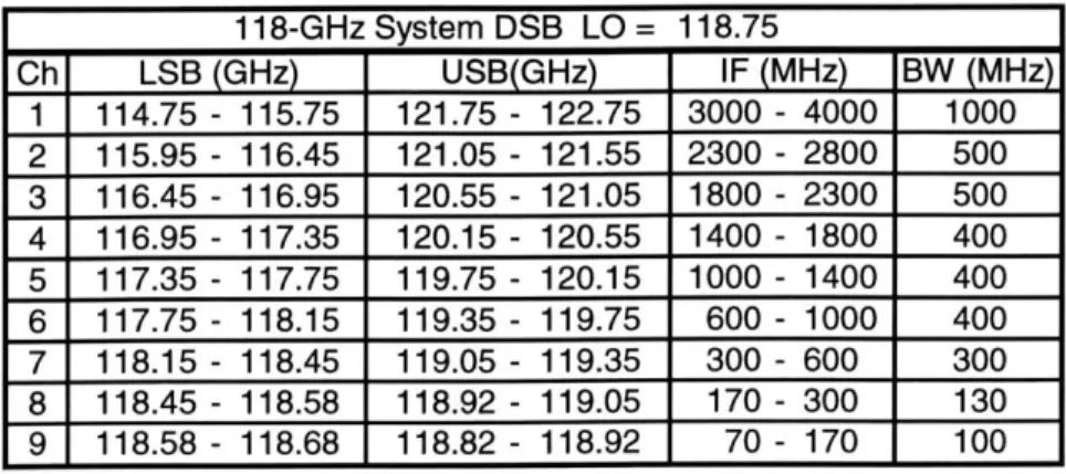
double sideband (DSB) super heterodyne receiver that has nine channels of which the first six are useable. A list of the channels and frequencies can be found in Table 3.1 and Table 3.2. For each
system, a weighting function is applied to each channel for the purpose of seeing a sounding from
NAST-M. From an altitude of 20 km, the nadir spatial resolution is 2.6 km. NAST-M has an
antenna reflector that scans ± 64.80 from nadir and makes 19 measurements with spacing of
The output from each receiver is a voltage value between ±10 volts. The voltage value is then
converted via A/D conversion to a value between ± 216 . After the conversion, it is saved to disk
as a "count". There are 25 spots total for which a count is saved. Two measurements are made
looking at the sky pipe (zenith), two are made looking at a hot load, one measurement is made for each of the 19 nadir spots, and two are made for the ambient load.
During the missions of CLOUDIOP, WVIOP, and AFWEX, NAST-M was mounted in a
superpod underneath the Proteus' fuselage. The Proteus is a custom built aircraft from Scaled Composite LLC. Two Williams International FJ44-2E turbofan engines were selected for propulsion. Its unique shape allows for many different configurations (Figure 3-1) for mounting instruments for various testbeds. The Proteus has a payload of up to 2000 pounds and can cruise at altitudes above 18 km for a maximum of 14 hours. Two crucial pieces of data supplied by the Proteus are the static air pressure and the aircraft roll. The static pressure will be used to provide NAST-M's relative height above the earth's surface. The aircraft roll will be used to determine the flatness of a scan. Previously, the aircraft roll was used take the rolls out of calibrated data so that the brightness temperatures measured would seem as though the aircraft was flying perfectly flat. But because of the location, NAST-M's sky pipe would be blocked off by the fuselage of the Proteus. An attempt to mount NAST-M with a 10 degree tilt to point away from the fuselage was unsuccessful. The fuselage was still in the way. By introducing a 10 degree tilt, a spot shift of the nadir views from previous missions CAMEX and WINTEX was inevitable. Without the zenith view, the calibration routine for the previous missions would have to be modified so that only the hot load and the ambient load counts will be used in calibrating brightness temperatures.
Table 3.1 Spectral Description of the NAST-M 54-GHz System.
54-GHz System SSB LO = 46 Ch RF (GHz) IF MHz BW (MHz 1 50.21 - 50.39 4210 - 4390 180 2 51.56 - 51.96 5560 - 5960 400 3 52.6 - 53 6600 - 7000 400 4 53.63 - 53.87 7630 - 7870 240 5 54.2 - 54.6 8200 - 8600 400 6 54.74 - 55.14 8740 - 9140 400 7 55.335 - 55.665 9335 - 9665 330 8 55.885 - 56.155 9885 - 10155 270
Table 3.2 Spectral Description of the NAST-M 118-GHz System. 118-GHz System DSB LO = 118.75 Ch LSB (GHz) USB(GHz) IF (MHz) BW (MHz) 1 114.75 - 115.75 121.75 - 122.75 3000 - 4000 1000 2 115.95 - 116.45 121.05 - 121.55 2300 - 2800 500 3 116.45 - 116.95 120.55 - 121.05 1800 - 2300 500 4 116.95 - 117.35 120.15 - 120.55 1400 - 1800 400 5 117.35 - 117.75 119.75 - 120.15 1000 - 1400 400 6 117.75 - 118.15 119.35 - 119.75 600 - 1000 400 7 118.15 - 118.45 119.05 - 119.35 300 - 600 300 8 118.45- 118.58 118.92- 119.05 170- 300 130 9 118.58- 118.68 118.82- 118.92 70- 170 100
Figure 3-1 Different Configurations of the Proteus.
3.1.1 Calibration
During calibration, the raw data recorded by NAST-M (counts), is linearly transformed into brightness temperature in a least squares sense. Using the Proteus as an aircraft testbed resulted in losing the zenith view calibration load. Only the hot and ambient loads remain for calibration. The scan pattern is still the same starting with two measurements of the zenith view, two
measurements of the hot load, one measurement for each of the 19 nadir views, and two
measurements of the ambient load. Each scan (all 25 spots) usually takes around 5.5 seconds to complete. During calibration, we simply ignore the zenith view counts. The calculated
brightness temperature can be modeled with the following formula:
Tb = g -C +b (3.1)
The gain g and baseline b can be derived by solving a set of linear equations using the
calibration points (CH, TH ) and (CA, TA ). The subscripts H and A represent the counts and
measured temperature in Kelvin of the hot and ambient load respectively. During flight, the temperatures of both loads are measured by the Resistive Thermal Device (RTD) unit [19] within
NAST-M. The solution for g and b is:
TA -TH
b=TA - CA -CHTA-TH CA (3.3)
b=,_A H
This calculation is made for each spot. The estimated gain and baseline are then used to convert the counts for each spot into brightness temperature. This process repeats all over for the next scan.
3.1.2 Correction for thermal gradients in the hot load
Since the hot load is heated to maintain an average temperature of 334K at all altitudes (roughly up to 16 km), the hot load may not be uniformly 334K throughout the blackbody. The hot load has 7 RTD's measuring its temperature. To compensate for such a gradient, hot load weights for each of the RTD's have been calculated to find the best average temperature for the hot load.
3.1.3 Antenna beam spillover correction
Side lobes of an antenna pattern can play a significant role in the measurement of radiances. For example, when the antenna is pointed at the hot load, radiation contributions from the sky view and the nadir view will add to radiance measurement. This additional corruption will offset the actual brightness temperature of the hot load. The hot load will appear to be warmer. The same will happen for the ambient load. The corrupted temperature of the ambient load and hot load can be modeled as a linear combination of the spillover through the sky pipe, the nadir view, and the "true" load temperature as:
T
=ZTZ +7 TN N +l-Z )qfA (34)T, =7Z TZ +7N N +( Z W H (3.5)
The four q values for each radiometer channel have been accurately measured in the lab. TZ and
TN can be estimated from NAST-M data. With these values, the true load temperatures can be
estimated along with the corruption corrected nadir brightness temperatures. More information can be found in appendix C of [19].
3.1.4 Instrument Sensitivity
Inherent to all systems is the presence of noise. The theoretical noise can be calculated from
A TRms ATRMS can be calculated directly by knowing the receiver temperature, target
temperature, bandwidth, integration time, and calibration error approximation. A different approach involves calibrating the counts and finding the standard deviation based on the calibrated brightness temperature on the calibration loads (Table 3.3). Actual measurements of the amount of standard deviation have been done in [18] and [19].
54-GHz System 11 8-GHz System Ch. 1 0.1879 Ch. 5 0.1248 Ch. 1 0.1922 Ch. 5 0.3002 Ch. 2 0.1274 Ch. 6 0.1528 Ch. 2 0.2436 Ch. 6 0.3814 Ch. 3 0.1084 Ch. 7 -0.1754 Ch. 3 0.2066 Ch. 7 0.6080 Ch. 4 0.1474 Ch. 8 0.2321 Ch. 4 0.2679 Oh. 8 0.8930 Ch. 9 1.1545
In training an estimator for temperature retrievals, the measurements can be used to simulate noise NAST-M would measure and added to simulated brightness temperatures.
3.1.5 Brightness Temperature Post Processing
In preparation of measured NAST-M data, two steps are made. Using Proteus navigational data, the aircraft roll is attempted to be removed. Anytime the aircraft roll more than 2 degrees, the brightness temperature value before and after the roll are interpolated to estimated the brightness temperature for that scan as if there were no roll.
The second step is to lessen the effects of noise. Smoothing of the data is performed with a triangular filter. This is accomplished by taking a boxcar and filtering the data for each spot, and for each channel. This result is then time reversed and filtered by the same boxcar. The final output is then time reversed to end up with filtered zero phased-shift brightness temperatures [20]. The boxcar filter is 4 samples long. The height of each sample is one over the length of the
filter, in this case .
3.2 TIGR profile set
The TIGR profile consists of a collection of 1761 temperature profiles [21]. Table 3.4 shows the distribution across climates. Each profile has been read into MATLAB using a script [appendix]. One profile contains 40 temperature measurements at 40 different pressure levels. Water vapor content has been calculated using [9]. Using these two measurements along with surface parameters, one can simulate brightness temperatures. Since NAST-M was flown at a mean pressure of 112 mbar during CLOUDIOP, WVIOP, and AFWEX, only the first 22 pressure levels will be attempted for retrieval. Each profile contains a surface temperature but it is only the surface air temperature. Since the retrievals will be done over land, a Gaussian random variable of zero mean and standard deviation of 3K will be added.
Number of Climate Type Radiosondes Tropical Atmosphere 322
Mid Latitude-1 Atmosphere 388
Mid Latitude-2 Atmosphere 354 Polar-i Atmosphere 104
Polar-2 Atmosphere 593
Table 3.4 Distribution of TIGR Profiles Throughout the Climates.
3.2.1 Simulating Brightness Temperature Components
Since training of an estimator will be performed using the TIGR set, a pre-computed set of
upwelling TbU,, downwelling Tb4d , and one way transmittance E have been calculated and
saved for future use. A MATLAB script to calculate these components can be found in the appendix. Anytime a set of brightness temperatures are needed for training or testing the performance of the estimator, a random set of surface emissivities, surface temperatures, and pressure levels of the instruments location above the earth can be generated to create a new
realization of simulated brightness temperatures T.sim
3.3 Atmospheric Radiation Measurement Program
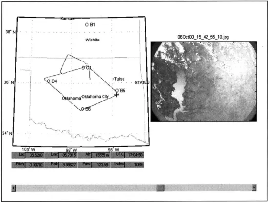
During each mission, a set of radiosondes and surface air temperature measurements have been collected for the days NAST-M was flown. This small ensemble of radiosondes can be obtained from the Atmospheric Radiation Measurement Program (ARM). The ARM program is setup to measure the many uncertainties of global climate change. The area in particular is the Southern Great Plains which is mainly located in Oklahoma and Kansas, USA. Figure 3-2 is an example of a typical NAST-M trajectory of the Southem Great Plains. The set of ARM data will serve as a means of truth so that retrieved data can be compared. ARM will also serve as a method of calibration for NAST-M data.
OBi 38'N WichIta -60ct00_15_42_55_10jpg 34Tu sa 3WN - TX Nahoma-Oklahoma City* 34 N 100 WW 96 W
Figure 3-2 Southern Great Plains and Radiosonde Sites.
3.3.1 Partial atmosphere vs. Entire Atmosphere
The collection of radiosondes to be used to characterize the atmosphere NAST-M flew over,
typically floated up to around the 2 2"d pressure level of the TIGR set. In the TIGR profile set,
there are 40 pressure levels that characterize an atmosphere. When computing T , , Tbd , and E,
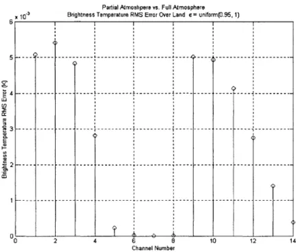
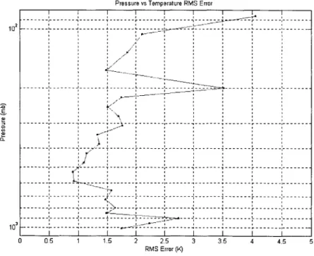
ideally one would like to use the entire Earth's atmosphere. The TIGR set captures most of the atmosphere to be modeled. To characterize the atmosphere using an ARM radiosonde for a particular day and to compare it to the TIGR set would require using only the first 22 pressure levels. The 22 pressure levels in the TIGR set and the collection of radiosondes are satisfactory because NAST-M was flown around the same pressure level. The RMS errors resulting from using a partial atmosphere and a full atmosphere is shown in Figure 3-3.
Partial Atmoshpere vs. Full Atmosphere
x 1- Brightness Temperature RMS Error Over Land e= uniform(.95, 1)
6 C) 3 w
0
2 4 6 6 10 12 14 Channel NumberFigure 3-3 Partial Atmosphere vs. Full Atmosphere.
3.3.2 Simulation of Brightness Temperatures from ARM
When collecting usable ARM radiosondes, certain conditions must be met.
1. Based on the trajectory NAST-M was flown, a radiosonde launch site must be within in
50 km.
2. The radiosonde must have 22 pressure levels that match up with the TIGR pressure levels.
3. The duration of the radiosonde flight must have some overlap with the duration of
NAST-M's flight.
It has been found that most of the ARM radiosondes collected begin floating from the surface to around the 22nd pressure level of the TIGR profile set. This works out great because the mean
pressure NAST-M was flown was also around the 2 2"d pressure level of the TIGR set. With this
small ensemble of radiosondes, brightness temperature components can be calculated. Using a partial atmosphere as opposed to a full atmosphere introduces very little error in calculating the
from the radiosondes in the same manner as the TIGR set, simulated brightness temperatures can be randomly generated by introducing a random set of surface parameters
3.4 CLOUDIOP, WVIOP, and AFWEX Deployments
Missions CLOUDIOP, WVIOP, and AFWEX occurred over the southern Great Plains area (OK and KS). In attempts to retrieve temperature for these missions, the assumption of no liquid content in the atmosphere will be used. Historically for this region, land surface emissivities have
ranged from 0.95 to 1. Also the surface emissivity of the 54-GHz is usually lower than the
118-GHz. To help model the surface emissivity of the 54-GHz, an emissivity value uniformly
distributed between 0.95 and 1 will be generated. A zero-mean Gaussian with standard deviation
0.01 will be added to add a little randomness. The 118-GHz surface emissivity is found by using
the following formula:
1 2
E118 =-+-E54 (3.6)
3 3
A zero-mean Gaussian with standard deviation of 0.01 is added to the emissivity of the 118-GHz.
This is important because during the training of an estimator, we don't want it to train to noise.
Of course the randomly generated emissivities will have to be clipped to 1 if they exceed this
value. The surface temperatures are generated by taking the first entry of each TIGR profile and adding a zero mean Gaussian random variable with a standard deviation of 3 K.
3.5
Bias removal
Throughout the flight of NAST-M, data will be measured at various pressure levels. When
NAST-M is at the nominal pressure level, the brightness temperatures that have been calibrated
from the raw counts will be similar to the simulated brightness temperatures from the ARM radiosondes. Brightness temperatures simulated from ARM radiosondes will be simulated from the same pressure level as NAST-M. This step will reveal that NAST-M brightness temperatures
are slightly different than ARM brightness temperatures. Since ARM data is considered to be "truth", a small gain and baseline adjust will have to be made. For a particular day, an average of
different nadir view brightness temperatures near the launch site of the ARM radiosonde will be chosen to represent the same atmosphere the ARM radiosonde floated through. ARM brightness temperatures will be simulated from the same pressure level as NAST-M for each view. The difference will then be calculated:
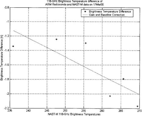
ATb,AN
b,ARM -Tb,NASTM (3.7)Having these differences, a scatter plot can be made. For each measured brightness temperature, the associated difference will be plotted i.e. the difference in brightness temperature is a function the measured NAST-M brightness temperature. The differences for each measured brightness temperature will be different and therefore a single line can't be calculated deterministically to
pass through all the points. The best solution is to find a gain g and baseline b of a linear
regression that fits the data the best. Figure 3-4 is an example of finding the best fit.
118-GHz Brightness Temperature difference of ARM Radiosonde and NAST-M data on 17MarO0
-0.8
+ Brightness Temperature Difference
- Gain and Baseline Correction
-1--- i--- T---
---c-1.28--- --- --- --- 1
235 240 245 250 255 260 265 270
NAST-M 1 18-GHz Brightness Temperatures
Figure 3-4 Example of Gain and Baseline Correction.
temporal differences between the flight portion and weather related anomalies of a radiosonde. The corrected NAST-M brightness temperature is as follows:
NA STM b,NASTM + ,AN
where:
AAN b
11B-GHz Brightness Temperature Correction of
NAST-M data on 17Mar0O
*)7f 265 260 ;-255 S250 S245 240 235 230 1.5 2 2.5 3 3.5 Channel Number 4 4.5 5 5.5 5.8) .9)
Figure 3-5 Example of Brightness Temperature Correction.
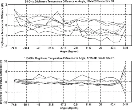
The gain and baseline calculations were found from the nadir view brightness temperatures. It can be shown that these calculations can be used for all angles. To show this, NAST-M
brightness temperatures have been simulated for all spots. Then a comparison between measured and simulated data was plotted. Figure 3-6 shows 54-GHz measured data from March 17, 00. Figure 3-7 is the plot of simulated data. The comparison is shown in Figure 3-10.
I I I II I
- ----~~~~- -- ---- - -- - -- -- --- - - -
--- - -
7--- ARM Brightness Temperature
NAST-M Brightness Temperature
Measured NAST-M 54-GHz Brighthness Temperature vs Angle
17MarO Sonde Site 81
270 -- ---;---;--- ----- --- 7---- --- --- ;---- -- ---Ch 1 Ch 2 260 -- ---- --- --- --- ---Ch 3 250 - - - - --- --- ---+--- - - - - - - --- L ---Ch 4 240 --- --- --- -- - --- ---E 240 230 ---- -- - - -I-- - - - -
~-
-74.0 -60.4 -46 -31 6 -17.2 -2.8 11.6 26 40.4 54 8 Angle (degree)Figure 3-6 Measured
54-GHz
data over all spots.Simulated NAST-M 54-GHz Brighthness Temperature vs Angle l7MlaOO Sonde Site 81
Ch3 250 - - - -Ch7 Ch 7 210 - - -- - --- --- - - ---- --- -- - - - -200 -74.8 -60.4 -46 -31.6 -17.2 -2.8 11.6 26 40.4 54.8 Angle (degree)
Figure 3-7 Simulated 54-GHz data over all spots.
Measured NAST-M 118-GHz Brighthness Temperature vs Angle
17MaOO Sonde Site B1
270--- --- ---2 6 0 - - - -- - - - - - --- - - - C h- -250 --- --- --- C2 -Ch3 S240 - - - - - - -
~
- -C-- -- - - - - - - - --- - h-A4 -E Ch5 230 -- - - --- I--- --- --- ---+- - - --- ---Ch6 220 --- --- ---210 -- --- - - - - - -200' 1 1 -74.8 -60.4 -46 -31.6 -17.2 -2.8 11.6 26 40.4 54.8 Angle (degree)Figure 3-8 Measured 118-GHz data over all spots.
Simulated NAST-M 118-GHz Brighthness Temperature vs Angle
17Mar0O Sonde Site 81
270 --- --- --- --- ---Ch 260 -- - r --- - --- --- - --- -- - - - - -- - --I ---Ch 2 250 -- - -*)-h 250 --- --- - - --- --- ---Ch 230 --- --- --- -- --- - -- --- - ---Ch 20 --- --- --- --- ---74.8 -60.4 -46 -31.6 -17.2 -2.8 11.6 26 40.4 54.8 Angle (degree)
Figure 3-9 Simulated 118-GHz data over all spots. 2 o E -1 g1 10 I-10-5
~
1054-GHz Brightness Temperature Difference vs Angle, 17Mar00 Sonde Site 81
I I I I I I I I
-74.8 -60.4 -46 -31.6 -17.2 -28 11.6 26 40.4 54.0
Angle (degrees)
118-GHz Brightness Temperature Difference vs Angle, 17Maro Sonde Site B1
- r - r - - - -
--74.8 -60.4 -46 -31.6 -17.2 -2.8 11.6 26
Angle (degrees)
40.4 54.8
Figure 3-10 Brightness Temperature Difference over all spots.
The flatness of each curve indicates that the offset of measured data from simulated data are similar across each spot. The small slope is the result of a roll from nadir of NAST-M while data was measured. Having shown that the offset is constant over all angles, gain and baseline
calculations can be found using the nadir view data.
3.5.1 Calculated Gain and Baseline
Gain and baseline calculations have been found for CLOUDIOP,
WVIOP,
and AFWEX. DuringCLOUDIOP, flight dates of Mar 17 00 and Mar 19 00 were chosen gain and baseline
calculations. During AFWEX, flight dates of Oct 04 00 and Oct 06 00 were chosen. For the AFWEX deployment, Dec 03 00 and Dec 06 00 were chosen. The results are as follows:
17-Mar-00 Radiosonde Site Location g54 b54 g118 b118 B1 -0.0056 1.4686 -0.0115 2.0393 B4 -0.0202 4.9562 -0.0260 5.0151 B5 -0.0282 6.9535 -0.0264 5.6557 B6 -0.0450 11.1659 -0.0223 5.1965 C1 -0.0121 3.1224 -0.0380 8.8195 Average: -0.0222 5.5333 -0.0248 5.3452
Table 3.5 Gain and Baseline Correction for 17 Mar 00.
19-Mar-00 Radiosonde Site Location g54 b54 g118 b118 B4 -0.1174 28.0051 -0.1130 26.7234 B5 -0.0535 12.8096 -0.0150 3.4008 B6 -0.0442 10.3140 -0.0223 3.3895 C1 -0.0260 6.4525 -0.0037 -0.1242 Average: -0.0603 14.3953 -0.0385 8.3474
Table 3.6 Gain and Baseline Correction for 19 Mar 00.
4-Oct-00
Radoso
1e
-0.1582
135.3658 1 -. 05
23.15151
Table 3.7 Gain and Baseline Correction for 04 Oct 00.
6-Oct-00 Radiosonde Site Location g54 b54 g118 b118 B4 -0.1402 32.0854 -0.0876 19.5942 B5 -0.0729 16.0016 -0.0526 10.4782 B6 -0.1141 25.6545 -0.072 15.155 C1 -0.1518 34.3656 -0.1445 33.453 Average: -0.1198 27.0268 -0.0892 19.6701
3-Dec-00
Radiosonde
II
Site Location
I
g54
I
b54
gl
g18b
18
Cl -0.0522 112.2324 10.0177 1-5.1402
Table 3.9 Gain and Baseline Correction for 03 Dec 00.
6-Dec-00
Site Location g54 Bs118 b54 bC 18
Radosn 1 -0.0639 115.9054 1-0.0247 16.4837