Publisher’s version / Version de l'éditeur:
Vous avez des questions? Nous pouvons vous aider. Pour communiquer directement avec un auteur, consultez la première page de la revue dans laquelle son article a été publié afin de trouver ses coordonnées. Si vous n’arrivez pas à les repérer, communiquez avec nous à [email protected].
Questions? Contact the NRC Publications Archive team at
[email protected]. If you wish to email the authors directly, please see the first page of the publication for their contact information.
https://publications-cnrc.canada.ca/fra/droits
L’accès à ce site Web et l’utilisation de son contenu sont assujettis aux conditions présentées dans le site LISEZ CES CONDITIONS ATTENTIVEMENT AVANT D’UTILISER CE SITE WEB.
15th International Symposium on Unmanned Untethered Submersible Technology
[Proceedings], 2007
READ THESE TERMS AND CONDITIONS CAREFULLY BEFORE USING THIS WEBSITE.
https://nrc-publications.canada.ca/eng/copyright
NRC Publications Archive Record / Notice des Archives des publications du CNRC : https://nrc-publications.canada.ca/eng/view/object/?id=02549b23-7c39-47a2-a766-3143f58f4e27 https://publications-cnrc.canada.ca/fra/voir/objet/?id=02549b23-7c39-47a2-a766-3143f58f4e27
NRC Publications Archive
Archives des publications du CNRC
This publication could be one of several versions: author’s original, accepted manuscript or the publisher’s version. / La version de cette publication peut être l’une des suivantes : la version prépublication de l’auteur, la version acceptée du manuscrit ou la version de l’éditeur.
Access and use of this website and the material on it are subject to the Terms and Conditions set forth at
Simulation of an underwater glider
SIMULATION OF AN UNDERWATER GLIDER
G. Stante
†, M. Nahon
†and C. Williams
‡ †Department of Mechanical Engineering, McGill University, Montreal, Canada
‡Institute for Ocean Technology, National Research Council, St. John’s, Canada
[email protected], [email protected], [email protected]
Abstract
Underwater gliders are being proposed as an alternative to the resource intensive and costly shipboard methods of oceanographic data collection. One such underwater vehicle currently in operation is the SLOCUM Glider. The purpose of the present work is to devise a dynamic simulation for the SLOCUM Glider that allows the vehicle’s motion to be predicted in response to control inputs. Such a simulation could be used to test operational scenarios and to aid in vehicle design. The simulation developed here relies on a component buildup method in which the hydrodynamics of the vehicle components (hull, wings, vertical fin) are estimated and summed. The simulation was validated against available experimental data. The agreement was reasonable, though it was determined that more precise information on the real vehicle was needed before further evaluations could be made. It was found that very small displacements of the vehicle C.G. had a substantial impact on the ensuing motion, and that the vehicle exhibited very stable behavior. Lateral oscillations observed in the real vehicle motion were attributed to an unmodeled interaction between the vehicle and its control system.
1.
Introduction
As an alternative to the resource intensive and costly shipboard methods of oceanographic data collection commonly practiced, unmanned underwater gliders are being proposed (Ref. [10]). In addition to being a cost-effective substitute, this type of vehicle could potentially be deployed for weeks, months or perhaps even years at a time collecting ocean data using onboard sensors and relaying the gathered information regularly via satellite or other communication link upon resurfacing. Deployed in large enough numbers, these vehicles would provide oceanographers and climatologists with a much larger and more accurate data set on ocean temperature, salinity and currents along with other ocean parameters of interest thereby enabling them to better understand and more accurately predict weather and climate phenomena. As such the development of underwater gliders is of great interest. Moreover, there is a need for dynamic simulations of these vehicles in order to aid in their general design, control and mission planning.
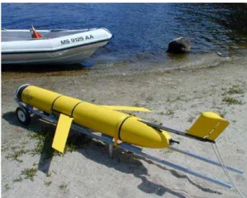
One such underwater vehicle which is currently in operation is the SLOCUM Glider, shown in Figure 1. The purpose of the present work is to devise a dynamic simulation for the SLOCUM Glider based on existing vehicle simulations developed and used at McGill
University. This report gives a description of the SLOCUM Glider Dynamic Simulation and contrasts its
performance with available mission data. Further, a mapping of the glider’s steady state characteristics and its performance in certain test cases based on simulation results are described along with suggestions for future improvements to the simulation.
Figure 1: SLOCUM glider on the beach
2 Vehicle Description
The SLOCUM Underwater Glider has a dry weight of 52 kg, has an overall length of 2.151 m and a hull diameter of 0.213 m. It features thin, swept and tapered flat plate wings and a similarly characterized fin mounted on a boom extending from the back of the main hull as seen in
Figure 1.
In addition to rudder control, this vehicle has the ability control its buoyancy within ± 250 g of neutral buoyancy using a buoyancy engine. Further, internal actuators enable the main battery pack to be shifted within ± 1 inch of its neutral location effectively shifting the glider’s center of gravity (C.G.). These control actions can be performed according to pre-programmed, sensor-based or external commands.
The glider’s operational scenario can be described as follows: the glider starts at the ocean surface where it obtains a GPS fix. The vehicle adjusts is rudder such that it follows a desired heading, renders itself negatively buoyant using its buoyancy engine to take in sea water ballast and moves its main battery pack (and hence its C.G.) forward such that the nose pitches downwards. The parameters are set such that these actions cause the vehicle to glide downwards at a prescribed sink rate, pitch and glidepath angle to a preset depth or sensor based altitude above the ocean floor. Once the desired depth is reached, the vehicle’s battery pack location (C.G. location) and buoyancy are adjusted such that the glider no longer increases its depth. After a prescribed linger time for data collection at depth, the vehicle renders itself positively buoyant by expelling sea water ballast and moving its battery pack location (C.G. location) aft. Once again, these parameters are set in a manner to cause the glider to glide upwards at a prescribed surfacing rate, pitch and glidepath angle. Upon reaching the surface, the vehicle obtains a new GPS fix and telemeters its data through an IRIDIUM satellite connection. Once the data transmission is completed, the glider compares its current location with its next preselected waypoint, adjusts its rudder position and dives anew. Currently, the autonomous endurance of the SLOCUM Glider is on the order of 4 weeks however it is envisioned that this time frame will increase to 2 years as subsequent versions of the vehicle or entirely new designs evolve [10] [11].
2.1
CAD Model
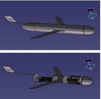
A 3D CAD model of the SLOCUM Glider was constructed using CATIA V5R17 in order to estimate the inertial characteristics of the vehicle, to map the location of its C.G. for different operating configurations, as well as to aid in the determination of its geometric data such as volume, surface area, etc. Figure 2 shows the external and internal arrangement of the CAD model.
Though every effort was made to include all of the glider’s components as well as to accurately estimate their mass and position, once completed, the digital mockup was approximately 5.6 kg underweight and its neutral C.G. position was ~43 mm fore and ~3 mm below the glider’s actual position. As such, a point mass of 5.6 kg was added in order to bring the CAD model inline with the glider’s characteristics.
The CAD model incorporates the movement of the main battery pack by ± 1 inch from its neutral position. However it must be noted that, the CAD model does not incorporate the movement of the actuator which moves the battery pack, the movement of the piston within the buoyancy engine which pumps in or expel sea water ballast or the sea water ballast itself. As such, the location of the glider’s C.G., its modeled mass and its inertia tensor for different operating configurations are
estimated by considering the movement of the main battery pack only.
Figure 2: CAD Model of the SLOCUM Glider
2.2
Parameters of Interest
The CAD model was used in order to estimate the inertia tensor of the vehicle at discrete positions of the main battery pack. It was found however that the inertia tensor varies very little over the range of motion of the battery pack. Hence the vehicle’s inertia tensor is taken to be constant within the simulation using the values for the neutral battery position configuration. Further, it is determined that the movement of main battery pack corresponds to a range of longitudinal C.G. locations of 0.0727 m to 0.0817 m as measured forward from the center of the glider’s main hull. The correlation between the battery pack position and the longitudinal location of the C.G. is shown in Figure 3.
Figure 3: Correlation Between Battery Position and CG Location
3
Vehicle Model
The dynamic model for the SLOCUM Glider is based on prior works in the modeling of AUVs and airships [1][2]. These works outline a component buildup approach to the dynamic modeling of vehicles which derive their lift via buoyancy, though they differ in the manner in which the equations of motion are formulated.
3.1
Equations of Motion
In order to develop the equations of motion for the
SLOCUM Glider, 2 reference frames are established. The
first is a body-fixed frame whose origin is set at the center of the vehicle’s main hull and oriented in the customary aeronautical manner, i.e. with the +x-axis pointing forward through the nose, the +y-axis outward through the starboard wing and the +z-axis pointing downwards. The second frame is the Newtonian (inertial) frame whose axes are oriented such that the +ZI
axis points downwards towards the ocean floor, i.e. in the direction of increasing depth. Using these frames, the vehicle’s position in space is described by the position vector from the origin of the inertial frame to the origin of the body frame, and its orientation is given by the 3 Euler Angles, i.e. roll (φ), pitch (θ) and yaw (ψ).
For the sake of convenience, the equations of motion are derived in the body-fixed frame using the Newton-Euler approach. They can be expressed in matrix-vector form as [2]:
I G Bu A H
=
+
+
+
+
Mq
&&
τ
τ
τ
τ
τ
(1) Where M is the mass matrix, q& contains the translational and angular velocities of the vehicle expressed in the body-fixed frame and the
τ
i’s are vectors comprised ofthe forces and moments due to a given phenomenon, including inertial (I), gravity (G), buoyancy (Bu), added mass (A) and hydrodynamic (H).
Once the equations of motion are formed, eq. (1) can be solved for
q
&&
as:(
)
1 I G Bu A H −=
+
+
+
+
q
&&
M
τ
τ
τ
τ
τ
(2) However, we are interested in the kinematic quantities of the glider expressed in the Newtonian frame. These parameters can be obtained from:
x
&
=
Tq&
(3)&&
x
=
Tq
&&
+
Tq
&
&
wherex
is a vector made up of the components of the position vector from the origin of the inertial frame to the origin of the body frame, and the three Euler Angles. The transformation matrixT
is obtained by considering thekinematic relationship between the time rate of change of the Euler Angles and the angular rates, as well as the rotation matrix which transforms a vector from the body-fixed frame to the Newtonian frame [1].
Once
&&
x
andx&
are obtained, they can be integrated numerically using any number of standard methods to yieldx&
and x at subsequent time steps over a given time interval.3.2
Inertial, Gravitational and Buoyancy
Forces and Moments
The inertial force and moment vector term
τ
I appearingin equations (1) and (2) incorporates centrifugal and Coriolis effects as well as those which arise due to the fact that the Newton-Euler Equations used in deriving equations (1) and (2) were written about the origin of the body-fixed frame and not the C.G. for the vehicle as is customarily done. Li [2] summarized the terms relating to the aforementioned effects.
The gravitational force acting on the glider can be expressed as a force in the inertial ZI direction that is
applied at the vehicle C.G. There is therefore a corresponding moment exerted due to the moment arm from the origin of the body-fixed frame to the C.G. The SLOCUM Glider’s geometry is designed such that it is essentially neutrally buoyant. Any imperfection in the vehicle’s neutral buoyancy and trim is corrected with the use of lead shot ballast. However the glider pumps in or expels sea water ballast (± 0.250 kg maximum) in order to change the vehicle’s buoyancy thus causing it to descend or ascend within the water column. The force and mass due to buoyancy effects can thus be written as
BU = (m + dBU)g where dBU is the mass of sea water
taken in or expelled. The buoyancy force is considered to act at the glider’s center of buoyancy (C.B.) and creates a corresponding moment due to the moment arm from the origin of the body-fixed frame to the C.B..
3.3
Hydrodynamic Force and Moment
The term
τ
H appearing in equations (1) and (2)represents the sum of all the hydrodynamic forces and moments acting on each of the glider’s surfaces, i.e. sw pw f B H x x x x sw sw pw pw f f B B
+
+
+
⎡
⎤
= ⎢
⎥
+
+
+
⎢
⎥
⎣
⎦
F
F
F
F
τ
r F
r F
r F
r F
(4) where the subscript sw refers to the starboard wing, pw to the port wing, f to the fin and B to the main body/hull of the glider. TheF
i’s are taken to be acting at theconstituent elements. Hence, the
r
i’s refer to theposition vectors of the aforementioned centers of pressure from the origin of the body-fixed frame, expressed in the body-fixed frame. Note that the forces acting on the vehicle’s fin boom are assumed negligible. In order to determine the hydrodynamic forces and moments acting on a body, one must consider the velocity of the body relative to the fluid. The local water velocity can be subtracted from the vehicle velocity in order to define velocities relative to the fluid.
3.3.1
Hydrodynamics Forces on the Wing
The wings of the SLOCUM Glider are swept, tapered and made up of flat plate aerofoils 2 mm thick, as seen in Figures 1 and 2. In order to account for the fact that the glider’s wings are swept and to more accurately capture their behavior at varying angles of attack and sideslip, we define 2 local wing body-fixed frames. Both of these frames are defined such that their origin is coincident with the origin of the body-fixed frame and that they are oriented along each of the wing’s sweep line. Thus the local frame for the starboard wing is obtained by rotating the body-fixed frame by the wing’s sweep angle Λw (44°)
about the z-axis. Similarly, the local port wing frame is obtained by rotating the body-fixed frame by -Λw about
the z-axis.
We can then determine the velocity of the center of pressure of each wing (relative to the fluid), express these in the local wing frames and use them to calculate the appropriate angles of attack and sideslip followed by the hydrodynamic lift and drag forces. The resultant forces must then be transformed back to the body-fixed frame and the moments which they cause accounted for. Further details on this process can be found in Ref. [12]. As mentioned at the beginning of Section 3.5.1, the wings of the SLOCUM Glider are swept and tapered flat plates. Unfortunately, no aerodynamic/hydrodynamic data for the glider’s wings or those of a similar configuration is currently available. As such, the hydrodynamic characteristics of the glider’s wings are taken to be those of finite rectangular flat plates. Ref. [3] presents such data for various plate aspect ratios at angles of attack ranging from 0 to 90° in 10° increments. However Ref. [3] does not provide the required data at aspect ratios above 3.0. Hence the data needed to be extrapolated based on various visible trends in the numbers in order to address the wing aspect ratio of 7.76. Using the data given in Ref. [3] and that generated via extrapolation, the wing lift and drag coefficients at a given angle of attack are determined by means of cubic splines.
Appearing in eq. (4) are the position vectors from the origin of the body-fixed frame to the center of pressure
of each wing, i.e.
r
swandr
pw. Due to the wing sweep and taper, the center of pressure of the wing no longer lies at the midpoint of the line through the center of pressures (aerodynamic centers) of the constituent aerofoil sections but is moved further back and inwards. Ref. [4] presents a method to determine the center of pressure of a swept, linearly tapered wing assuming that the slope of the 2D lift curve is constant and that the spanwise load distribution is elliptic.It is assumed that the SLOCUM Glider’s wings meet the above criteria for the majority of its operating conditions..
3.3.2
Hydrodynamics Forces on the Fin
The fin of the SLOCUM Glider is also a swept and tapered flat plate 2.8 mm as shown in Figures 1 and 2. As such, we proceed in an analogous manner to that presented for the wings in order to determine the hydrodynamic forces acting on the fin. As was the case with the glider’s wings, we define a local body-fixed frame for the fin such that it is oriented along the fin’s sweep line and its origin is coincident with the origin of the body-fixed frame. Hence the fin frame is obtained by rotating the body-fixed frame by the fin’s sweep angle Λf
(30°) about the y-axis. Further, as was done for the wing, the velocity of the fin’s center of pressure (relative to the fluid) must be determined, expressed in the local fin frame, and used to calculate the angles of attack and sideslip as well as the hydrodynamic lift and drag forces. The resultant force must then be transformed back to the body-fixed frame and the moment which it causes taken into account. The incremental increase (decrease) in the fin lift and drag coefficients due to rudder deflection are estimated using the method outlined by Li [2]. Further details may be found in [12].
As previously mentioned, along with the wings, the
SLOCUM Glider’s fin is a swept and tapered flat plate.
Hence the hydrodynamic characteristics of the glider’s fin are approximated in the same manner as for the wing. Here however, the data given in Ref. [3] already encompassed the fin’s aspect ratio of 0.927 thus no extrapolation was necessary. The hydrodynamic data is interpolated using cubic splines in order to determine the fin lift and drag coefficients at a given angle of attack (i.e. the fin’s sideslip angle).
As previously discussed, the fin of the SLOCUM Glider is also a swept and tapered flat plate. Hence the method used to determine the glider’s fin C.P. is essentially identical to that used to determine the centers of pressure of the wings. Only superficial changes required to modify the approach in order to tailor it to the fin [12].
3.3.3
Hydrodynamics Forces on the Hull
The hydrodynamic forces acting on the hull are determined in an analogous manner to those described for the glider’s wings and fin. Here however, we need
not define a new coordinate frame and the velocity of the hull’s center of pressure expressed in the body-fixed frame can be used directly to determine the hull’s angle of attack and sideslip as well as the lift and drag forces acting on the hull.
The hydrodynamic lift and drag coefficients of the
SLOCUM Glider’s hull/main body are calculated as
summarized in Ref. [1]. The location of the center of pressure of the hull is dependent on the glider’s velocity and the hull’s angle of attack. As such it is not fixed. The method used to determine the hull’s C.P. used here is based upon the work of Evans (Ref. [7]).
3.4
Added Mass Effects
Added mass effects arise due to pressure-induced fluid-structure interactions. The force and moment that these effects induce is accounted for by the method suggested in Ref. [2]. The Added Mass Matrix, MA, is a 6 x 6
matrix encompassing the added mass effects of the hull/body, the wings and the fin. It is assumed here that added mass contribution of the fin boom is negligible. Thus MA consists of contributions due to the hull, wings
and fins.
The added mass of the hull can be estimated as suggested in Ref. [2] by approximating the hull/main body of the
SLOCUM Glider as an ellipsoid. For an ellipsoid, it can
be shown that the off-diagonal terms in its added mass matrix are zero provided that the body-fixed frame has its origin at the center of volume (C.V.) of the ellipsoid and it is oriented such that the x-axis lies on the major axis of the ellipsoid, the y-axis on its minor axis and the z-axis pointing downwards. Since the glider’s body-fixed frame is so oriented and, assuming that C.V. of the hull approximating ellipsoid is only marginally offset longitudinally from the origin of the frame, the off-diagonal terms in the added mass matrix of the hull, MAB,
can be essentially taken as zero. The diagonal terms of
MAB can be expressed as described in Refs. [8] and [9].
Since most underwater vehicles have short and stubby fins, only the added mass of the hull is typically considered. However, the wing span of the SLOCUM
Glider is comparable to the length of its main hull thus
ignoring the added mass effect of the wings is inadvisable. Given that the wings are thin, the added mass effects in the x and y directions are negligible. By the same token, the added mass moment in yaw is also negligible. Moreover, given the position of the wings, the moment arm in pitch is very nearly zero hence the added mass effects in the pitch direction are also negligible. In order to facilitate the estimation of the added mass of the wings, they are approximated as right, circular cylinders whose center lines extend outward from the centers of the root chord of the exposed wings. Therefore, the length of the cylinders is given by
B w
w D
b
l = −
2 (where bw is the tip-to-tip wing span) and
their radii are taken to be half the wing’s average chord length, i.e. 2 w w c r = .
As with the glider’s wings, SLOCUM’s fin is of sufficient dimension that its added mass effect cannot be neglected. Since the fin is thin, the added mass effects in the x and z directions are negligible. By similar consideration, the added mass moment in pitch is also negligible.
As with the wings, the fin is approximated as a right, circular cylinder whose center line extends outward from the center of the fin’s root chord. Hence, the length of the cylinder is taken as the span of the fin, i.e. lf = bf, and its
radius is taken as half the fin’s average chord length, i.e.
2 f f c r = .
3.5
Implementation
The dynamic model as outlined above was implemented in MABLAB 7.1 using its ode45 command to integrate the equations of motion. The structure of the code and method of solution was essentially identical to that outlined in [1].
The inputs to the simulation consist of the glider’s buoyancy, the position of the battery pack and the rudder deflection. All these can be specified as functions of time. The outputs of the simulation consist of the glider’s motion, as represented by its translational and rotational position, velocity and acceleration.
4
Simulation Results
4.1
Mission Data
To assess the performance of the simulation, mission data from a sortie of 18.2 hours off the coast of Newfoundland was used. This data was made up of 44 dive and climb segments with intermediate loitering at depth and on the surface interspersing them. The initial comparison to the simulation focused on steady dive or climb cases. We therefore selected segments that had essentially constant sink (climb) rate, pitch angle, battery position and ballast pumped throughout the dive or climb. Although a constant heading angle and zero rudder deflection and roll angle would have been desirable, no segment could be found with these latter features. Rather, all segments contained significant oscillatory yaw motion and rudder action, and some small oscillatory roll motion. As such, the baseline segments selected were those where the rudder deflection oscillated with peak to peak amplitude of less than 20o.
Figure 4: Climb 12; A Typical Steady Climb
All told, we identified 9 climbs and 9 dives that satisfied our desired conditions. An example of one of these (Climb 12) is presented in Figure 4. To circumvent the noise in the measured data, the signals were averaged over the duration of the segments in order to compare them with the simulation predictions. From the 9 climbs and 9 dives, we selected two of each (Climbs 29 and 36; and Dives 23 and 25) for initial validation. Each pair exhibited substantially the same conditions, as shown in Tables 2 and 3.
The values of xCG shown in the tables are expressed in
the body-fixed frame and are determined from the average battery position using the correlation shown in
Figure 3. Further, the xCG mission values vary, on
average, less than 1 mm from the glider’s neutral longitudinal C.G. position of xCG = 77 mm which is well
within the possible xCG displacement of ±4.5 mm (caused
by the possible main battery pack movement of ± 1 inch). The incremental changes in buoyancy, dBU, in the table are determined by converting the recorded average
sea water ballast pumped in or expelled (in cc) into kilograms using the density of sea water.
Table 2: Climb Comparison
Case Climb xCG (mm) dBu (kg) Avg. Pitch Angle (deg) Avg. Climb rate (m/s) 29 76.142 0.24044 27.4 -0.243 36 76.124 0.24034 27.5 -0.242 Exp Avg 76.133 0.24039 27.4 -0.243 Sim 76.130 0.24000 19.2 -0.203 Table 3: Dive Comparison
Case Dive xCG (mm) dBu (kg) Avg. Pitch Angle (deg) Avg. Dive rate (m/s) 23 78.131 -0.23969 -27.0 0.190 25 78.155 -0.23930 -26.9 0.188 Exp Avg 78.143 -0.23950 -27.0 0.189 Sim 78.140 -0.23900 -23.6 0.263
4.2
Corresponding Simulation Response
As a starting point for simulation performance assessment, the simulation was run using the average of the xCG and dBU values for the two climbs and the two
dives highlighted above. This was done in order to determine if the simulation accurately predicts the glider’s steady state pitch and sink (climb) rate in climb and dive. During these runs, the rudder angle was set to zero and the sea was modeled as a quiescent fluid since no information on currents is currently available. The only kinematic variables available for comparison are the sink/climb rate (Z&I), the pitch angle (θ), the roll angle (φ) and the heading/yaw angle (ψ). It was observed that using the average values of xCG = 76.13 mm with dBU =
0.240 kg in climb and xCG =78.14 mm with dBU = -0.239
kg in dive caused very little motion in any direction, let alone of the magnitude observed in the field data (Tables
2 and 3). This discrepancy can, at least partially, be
reconciled by noting the shortcomings in the pinpointing of the glider’s C.G. location. The nominal vertical (z) separation distance between the glider’s center of buoyancy (C.B.) and its C.G. is not precisely known but rather is estimated to be 6 mm after having ballasted and trimmed the glider. It is therefore plausible that this estimate is off by several millimeters in either direction. Moreover, the glider’s sensors sense the position of the main battery pack, not the xCG of the glider. The xCG is
determined based on the correlation developed using the devised CAD model of the glider which is currently incapable of taking into account factors which likely
affect the longitudinal position of the C.G.. Hence the average xCG values used in these initial tests and quoted
in Table 2 and 3 may be in error. Furthermore, it was determined that changing the glider’s xCG and/or zCG by
as little as a millimeter has significant impact on the simulated motion. Thus, a more precise estimation of the glider’s C.G. location and a more accurate model of how it shifts during the glider’s operation are essential in order to verify the simulation’s true accuracy.
Due to these shortcomings, the zCG location was varied in
an effort to discern the glider configurations in dive and in climb which best match the experimental data. It was found that a zCG = 3 mm (as opposed to 6 mm) led to the
best agreement with the mission data for the average xCG
values of xCG = 76.13 mm in climb and xCG = 78.14 mm
in dive. Using these parameters and the average dBU values quoted above, the simulation yielded the results shown in Tables 2 and 3.
Given the various uncertainties present in the model, there is a reasonable agreement between the simulation and experiment---the simulation returns results which are in the vicinity of those measured in the field. The simulated pitch angles are somewhat lower than those observed experimentally, while the simulated depth rate is lower in climb, and higher in dive. Based on this, it was considered reasonable to use the simulation to study the motion characteristics of the SLOCUM Glider. For the remainder of this paper, the terms “average climb simulation/glider configuration” and “average dive simulation/glider configuration” refer to the parameter settings of xCG = 76.13 mm and dBU = 0.240 kg for a
climb case and xCG = 78.14 mm and dBU = -0.239 kg for
a dive scenario. Moreover, the vertical location of the glider’s C.G. is taken as zCG = 3 mm in order to better
reflect the real performance of the glider as discussed above. In addition, since no information on ocean currents is currently available, the sea will be treated as a quiescent fluid throughout the remaining discussions.
4.3
Steady State Glider Performance
In an effort to better understand the effects of the glider’s center of gravity and the change in buoyancy, the simulation was run with various combinations of xCG
and dBU and the resultant steady state motion was recorded. For negative dBU values, xCG was varied from
its neutral xCG location to its fore limit, corresponding to
a dive scenario. For positive dBU values, xCG was varied
from its aft limit to the neutral position, representing a climb case. These were considered to constitute the normal operating envelope of the vehicle.
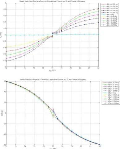
Figure 5 shows the resulting steady state sink (climb)
rate and pitch angle, as functions of xCG and dBU. We
observe a symmetry about the neutral C.G. location of
xCG = 77 mm. As expected, the constant dBU curves fan
out as the xCG is shifted away from its neutral position
illustrating a corresponding increase in Z&I. Moreover, the magnitude of Z&Iincreases as the magnitude of dBU
increases in both the climb and dive configurations as expected. By contrast, the steady state pitch angle seems little affected by variations of dBU, and seems to change only due to variations in the C.G. location. It is also noteworthy to mention that, though the results presented in Figure 5 were obtained using zCG = 3 mm, the same
trends are visible when using zCG = 6 mm.
Figure 5: Steady-State Depth Rate and Pitch Angle with Varying CG Position and Buoyancy Change
4.4
Transient Response
The preceding analysis did not include any closed loop control. However, the real glider is equipped with a proportional heading angle controller which controls t he vehicle’s rudder deflection according to
) ( desired actual p
control k σ σ
δ = − where σ denotes the heading angle. Using the mission data, the controller gain is estimated to be kp = 0.5 deg/deg by examining the
ratio of the heading and rudder deflection oscillations. Furthermore, since the heading angle is essentially the yaw angle ψ, the control law is implemented as
) ( desired actual p
control k ψ ψ
As a first test case of the glider’s transient behavior, we examine its response to a rudder pulse. The total rudder deflection is given by δ = δpulse + δcontrol where δpulse =
36º for 15 ≤ t ≤ 16 seconds. A positive rudder deflection is one which causes the glider to turn to starboard, i.e. in the +y direction. The desired heading/yaw angle is ψdesired = 0 throughout the simulation. Figure 6 shows the
simulation results for the average climb case.
Figure 6: Simulated Steady Climb with Rudder Pulse
We note that all of the motion variables return to their initial steady state values after the pulse, save the YI
displacement. The controller is responsible for returning
I
X& , Y&I and ψ to zero since, without the controller, they
maintain an offset. The heading angle controller also returns the vehicle to steady state more quickly than without the controller. An important observation is that the vehicle exhibits highly damped behavior, without indication of the oscillatory motions observed in the experimental data. This implies that, if the oscillations are due to a controller – ‘airframe’ interaction, then the relevant features of the controller (e.g. time delay or actuator dynamics) have not been captured here.
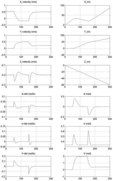
In the second test case, we examine the effect of a heading command change. The rudder control law is again taken as δcontrol =kp(ψdesired −ψactual) with kp =
0.5 degree/degree. The desired heading/yaw angle is set to ψdesired = 0 for t < 50 seconds, then to ψdesired = 110°
for 50 ≤ t ≤ 150seconds and then to ψdesired = 23° for t >
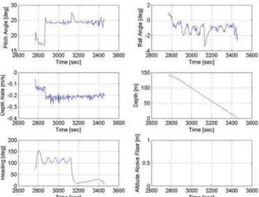
150 seconds. Figure 7 shows the vehicle’s simulated behavior in an average climb configuration. As a comparison, Figure 8 shows an actual heading change from 110o to 23o during a climb (Climb 2).
Figure 7: Simulated Steady Climb with Step Change in Desired Heading
Comparing Figures 7 and 8, we see that the simulation predicts a very similar vehicle yaw response while the glider undergoes a heading change from 110o to 23o. It is evident however that the simulation does not capture the oscillations about the desired heading/yaw angle visible in Figure 8. Examining the data for the climb in question, we find that the rudder is undergoing continuous oscillations before and after the heading change (not shown here).
Figure 8: Measured Steady Climb with Step Change in Desired Heading
5
Conclusions and Recommendations
The simulation results presented in Section 4 indicate that the simulation predicts the general motion trends observed in the baseline data. Moreover, the magnitudes of the predicted motion variables are in the vicinity of those of the actual glider. The simulation indicates that the vehicle’s natural motion is highly damped. However, the experimental data indicates the presence of a continual lateral oscillation, which we attribute to an interaction between the vehicle and its controller. We were not able to reproduce this oscillation in the simulation, and expect that this is due to an unmodeled aspect, such as time delay or phase lag.
As mentioned earlier, the true performance of the simulation cannot further evaluated before addressing the gaps in information regarding the glider’s C.G. location and its longitudinal migration as the glider is in various modes of operation. Moreover, the accuracy of this information is of paramount importance since millimeter changes in the C.G. location have a significant impact on the vehicle’s performance. Future work will therefore focus on generating more precise drawings of all the vehicle’s constituent components along with their individual masses and centers of gravity so that the CAD model is as accurate as possible. Moreover, the zCG of the
actual vehicle should be ascertained and used in the simulation. In addition, ocean current data should be obtained during experimental testing and integrated into the simulation.
References
[1] M. Nahon, “A Simplified Dynamics Model for Autonomous Underwater Vehicles”, IEEE Paper 0-7803-3185-0/96, 1996.
[2] Y. Li & M. Nahon, “Simulation of Airship Dynamics”, Proceedings of the AIAA Modeling and Simulation Technologies Conference, Keystone, 2006. [3] R. D. Blevins, Applied Fluid Dynamics Handbook, Van Nostrand Reinhold Company Inc., 1984.
[4] B. A. McCormick, Aerodynamics, Aeronautics, and
Flight Mechanics, J. Wiley & Sons, 1995, Chapter 3, 4.
[5] B. A. McCormick, Aerodynamics, Aeronautics, and
Flight Mechanics, J. Wiley & Sons, 1995, p. 100.
[6] Fink, USAF Stability and Control DATCOM, 1978, Section 4.1, 4.2 and 6.1.4.
[7] J. Evans, “Dynamic Modeling and Performance Evaluation of an Autonomous Underwater Vehicle”, M.Eng. Thesis, McGill University, 2003.
[8] T. I. Fossen, Guidance and Control of Ocean
Vehicles, John Wiley & Sons, New York, 1998.
[9] H. Lamb, Hydrodynamics, 6th Ed., Dover, New York, 1945.
[10] R. Bachmayer, N. Ehrich Leonard, J. Graver, E. Fiorelli, P. Bahatta and D. Paley, “Underwater Gliders: Recent Developments and Future Applications”, 2004
IEEE International Symposium on Underwater Technology, Taipei, Taiwan, April 2004.
[11] D. C. Webb, P. J. Simonetti and C. P. Jones, “SLOCUM: An Underwater Glider Propelled by Environmental Energy”, IEEE Journal of Oceanic
Engineering, Vol. 26, No. 4, October 2001.
[12] G. Stante, “Dynamic Simulation of the SLOCUM Glider”, M.Eng Project Report, McGill University, 2007.