Hydrogen-helium mixtures in the interiors of giant planets

Publisher’s version / Version de l'éditeur:

Physical Review B, 75, 2, 2007-01-11

READ THESE TERMS AND CONDITIONS CAREFULLY BEFORE USING THIS WEBSITE.

https://nrc-publications.canada.ca/eng/copyright

Vous avez des questions? Nous pouvons vous aider. Pour communiquer directement avec un auteur, consultez la première page de la revue dans laquelle son article a été publié afin de trouver ses coordonnées. Si vous n’arrivez pas à les repérer, communiquez avec nous à PublicationsArchive-ArchivesPublications@nrc-cnrc.gc.ca.

Questions? Contact the NRC Publications Archive team at

PublicationsArchive-ArchivesPublications@nrc-cnrc.gc.ca. If you wish to email the authors directly, please see the first page of the publication for their contact information.

Archives des publications du CNRC

This publication could be one of several versions: author’s original, accepted manuscript or the publisher’s version. / La version de cette publication peut être l’une des suivantes : la version prépublication de l’auteur, la version acceptée du manuscrit ou la version de l’éditeur.

For the publisher’s version, please access the DOI link below./ Pour consulter la version de l’éditeur, utilisez le lien DOI ci-dessous.

https://doi.org/10.1103/PhysRevB.75.024206

Access and use of this website and the material on it are subject to the Terms and Conditions set forth at

Hydrogen-helium mixtures in the interiors of giant planets

Vorberger, J.; Tamblyn, I.; Militzer, B.; Bonev, S. A.

https://publications-cnrc.canada.ca/fra/droits

L’accès à ce site Web et l’utilisation de son contenu sont assujettis aux conditions présentées dans le site LISEZ CES CONDITIONS ATTENTIVEMENT AVANT D’UTILISER CE SITE WEB.

NRC Publications Record / Notice d'Archives des publications de CNRC:

which leads to more stable hydrogen molecules compared to pure hydrogen for the same thermodynamic conditions. The ab initio treatment of the mixture enables us to investigate the validity of the widely used linear mixing approximation. We find deviations of up to 8% in energy and volume from linear mixing at constant pressure in the region of molecular dissociation.

DOI:10.1103/PhysRevB.75.024206 PACS number共s兲: 61.20.Ja, 61.25.Em, 61.25.Mv, 61.20.⫺p

I. INTRODUCTION

The discovery of the first extrasolar planet in 1995共Ref. 1兲 marked the beginning of a new era in planetary science, which is characterized by great improvements in observa-tional techniques and a rapidly expanding set of known ex-trasolar planets. Most of the about 200 known planets are giant gas planets in small orbits since the primary tool for detection, radio velocity measurement, is most sensitive for finding heavy planets that rapidly orbit their parent star.2,3 From radius measurements of transient extrasolar planets, we know that most of the discovered planets consist primarily of hydrogen and helium. Therefore, there is a great need for accurate equation of state共EOS兲 data for these elements un-der giant gas planet conditions.4 _{Knowledge of the} equilib-rium properties of mixtures of hydrogen and helium will help to clarify questions concerning the inner structure, origin, and evolution of such astrophysical objects. Open questions are whether or not hydrogen and helium phase separate in-side giant planets, whether or not a plasma phase transition72 under the influence of helium can be found, and whether or not a solid rocky core exists in Jupiter.4,5

The EOS of hydrogen has attracted considerable attention, and a large number of models have been introduced to char-acterize hydrogen at high pressure and temperature. Of great use in astrophysical calculations and planet modeling are 共free energy兲 models operating in the chemical picture.6–13_In these models, the hydrogen fluid is assumed to be composed of well-defined chemical species like atoms, molecules, and free charged particles. Such methods operate in the thermo-dynamic limit and are capable of describing large parameter regions of temperature and density. Further advantages of the free energy models are the small computational effort re-quired to calculate the EOS and explicit knowledge of all the considered contributions to the EOS. Ionization and dissocia-tion degrees are computed by means of mass acdissocia-tion laws and are not subject to fluctuations due to technical issues as in simulations. Atoms and molecules are treated as separate el-ementary species instead of being considered as bound states of electrons and nuclei. This implies certain approximations

that limit the quality of these approaches. At sufficiently high density, the definition of atoms and molecules becomes im-precise as the lifetime of such objects decreases rapidly with density and mean distances between nuclei and electrons be-come comparable to bond lengths.

In this paper, special emphasis will be placed on testing the accuracy of the linear mixing approximation, which is often applied in free energy models to calculate the EOS of mixtures of different chemical species such as hydrogen and helium. A similar approach can be used to characterize mix-tures of hydrogen atoms and molecules.8,14_This approxima-tion allows the calculaapproxima-tion of thermodynamic variables of mixtures by a simple linear superposition of properties of pure substances. Linear mixing is a useful assumption to make if reliable experimental or theoretical data are only available for pure substances or for cases where it has been shown that particles interact only weakly.

To avoid the shortcomings of chemical models, first-principles calculations can be applied. Such methods work in the physical picture and treat electrons and nuclei as elemen-tary particles interacting via the Coulomb potential. Quan-tum theory then describes the effects leading to the formation of atoms or molecules and their statistics. For hydrogen, there have been great efforts to study the equilibrium prop-erties by means of density functional theory 共DFT兲,15–17 DFT-molecular dynamics共DFT-MD兲,18–20 DFT–hypernetted-chain-equation combination 共DFT-HNC兲,21–23 _{path integral} Monte Carlo共PIMC兲,24,25

coupled electron-ion Monte Carlo 共QMC兲,26_{and Green’s function theory.}27,28

Questions addressed include the problem of the hydrogen Hugoniot29–32_{and helium Hugoniot,}33_{the nature of the} tran-sition in hydrogen from a molecular to an atomic state,24,34,35 the melting line of hydrogen,36the different molecular solid phases,17,37–39_{and the atomic solid共metallic Wigner crystal兲} proposed to be found at very high pressures.40–42_Although DFT-MD is primarily an electronic ground-state method, it can be readily applied to describe dense solid and fluid hy-drogen and helium at conditions relevant to giant gas planets because the electrons in such systems are either chemically bound or highly degenerate.

To our knowledge, there are only a few first-principles calculations dealing with the question of the helium influ-ence on the hydrogen EOS. Klepeis et al.16_{made predictions} concerning the hydrogen-helium phase separation but the DFT method applied in that paper is not suitable to treat the high-temperature liquid found inside giant gas planets since only lattices could be discussed. The first DFT-MD calcula-tions, performed by Pfaffenzeller et al.,43 _{lead to more} rea-sonable values for hydrogen-helium demixing. Their simula-tions were performed using Car-Parinello MD共CP-MD兲. The high-temperature region共T 艌 15 000 K兲 where partial ioniza-tion occurs was considered by Militzer.45

Here we present results concerning the hydrogen and hydrogen-helium EOS for conditions inside giant gas planets as derived from first-principles DFT-MD. We use Born-Oppenheimer MD 共BO-MD兲 in order to ensure well-converged electronic wave functions at every step. The den-sity and temperature values chosen cover the region of molecular dissociation where we expect corrections to the linear mixing approximation to be most significant.

We continue with Sec. II which contains details of our computational method. Results for the hydrogen EOS are presented in Sec. III A and compared to EOS data from a variety of other approaches. Furthermore, the ionic and elec-tronic structures of the hydrogen fluid and their dependence on temperature and density are investigated as well. The EOS and properties of hydrogen-helium mixtures are studied in Sec. III B. The focus there is on understanding how the presence of helium influences the stability of hydrogen mol-ecules and the electronic structure, as well as on determining excess mixing quantities. Finally, the validity of the linear mixing approximation is examined in Sec. III C, and Sec. IV provides a summary of our results and conclusions.

II. METHOD

We use first-principles DFT-MD within the physical pic-ture to describe hydrogen-helium mixpic-tures under giant gas planet conditions. This means that protons as well as helium nuclei are treated classically. Nuclei and electrons interact via a Coulomb potential. Since T Ⰶ TF, where TFis the Fermi temperature, for all densities and temperatures found inside a typical giant gas planet, we employ ground-state density functional theory to describe the electrons in the Coulomb field of the ions. The ions have sufficiently large mass to be treated as classical particles and their properties described well by means of molecular dynamics simulations. We em-ploy the Born-Oppenheimer approximation to decouple the dynamics of electrons and ions. The electrons thus respond instantaneously to the ionic motion and the electronic wave functions are converged at every ionic time step.

Compared to Car-Parinello MD, Born-Oppenheimer MD reliably keeps the electrons in their ground state without the necessity to use an artificial electron thermostat for systems with a small band gap. Moreover, it was recently shown that without a full reoptimization of the electronic wave functions in every step共as in CP-MD兲, the degree of dissociation can be artificially enhanced and the molecular to non-molecular transition is sped up.44

The calculations presented in this article were carried out with the CPMDpackage46 _{using the BO-MD mode. All MD} results were obtained within the N-V-T ensemble. A Nosè-Hoover thermostat was applied to adjust the system tempera-ture. The thermostat was tuned to the first vibration mode of the hydrogen molecule 共4400 cm−1_{兲. All DFT-MD} simula-tions were with 128 electrons in supercells with periodic boundary conditions, and convergence tests were performed with larger cells. An ionic time step of ⌬t = 16 a.u. 共1 a.u. = 0.0242 fs兲 was used throughout; however, we found that ⌬t = 32 a.u. is already sufficient for rs艌 1.86 in the hydrogen-helium mixtures关rs= 3 /兵共4␲n兲1/3aB其, where rsis the Wigner-Seitz radius and n the number density of electrons per unit volume兴. All simulations were run for at least 2 ps, and for the calculation of thermodynamic averages, such as pressure and energy, an initial time span of at least 0.1 ps was not considered to allow the system to equilibrate.

The DFT calculations were performed with plane waves up to a cutoff energy of 35–50 Ha, the Perdew-Burke-Ernzerhof generalized gradient approximation47 共GGA兲 for the exchange-correlation energy, and ⌫-point sampling of the Brillouin zone. We used local Troullier-Martins norm-conserving pseudopotentials.48,49 _{The pseudopotentials were} tested for transferability and for reproducing the bond length and ground-state energy of single hydrogen molecules as well as of helium dimers.

For each density, the simulations were started at low tem-perature where the system is in a molecular phase and the temperature was increased in steps of ⌬T = 500 K in order to avoid the premature destruction of molecules by temperature oscillations introduced by the thermostat.

The electronic densities of states 共DOS兲 were calculated for snapshots from MD simulations with the ABINIT

package50and using a Fermi-Dirac smearing. The presented results for DOS and band gaps are based on multiple snap-shots for each parameter set.

Finite-size effects were tested for by carrying out simula-tions with supercells containing up to 324 electrons共plus the required neutralizing number of protons and helium nuclei兲. For densities corresponding to 1.86艌 rs艌 1.6 and at T = 500 K we found the changes in pressure and energy to be smaller than 2%. The convergence of the Brillouin zone sam-pling was checked by optimizing the electronic density of several MD snapshots with ⌫ points and a 2 ⫻ 2 ⫻ 2 and a 4 ⫻ 4 ⫻ 4 Monkhorst-Pack grid of k points51 _{for a N}

e= 128 system. The Brillouin zone appears to be sufficiently small so that deviations between results with 1, 8, and 64 k points are below 1%共rs= 1.6, T = 500 K兲.

We also examined the significance of electronic excita-tions for the thermodynamic properties of the studied fluids. Snapshots from MD trajectories were taken and electronic states were populated according to a Fermi distribution cor-responding to the MD temperature. For rs= 2.4 and T = 7000 K the pressure was found to increase by 8%. Since the degeneracy parameter of the electrons increases while moving along an isentrope to the center of a giant gas planet, this can be considered an upper limit for finite-temperature electronic excitation effects; the error for higher densities and lower temperatures will be much smaller.

III. RESULTS

Here we present ab initio results for equilibrium proper-ties of hydrogen and hydrogen-helium mixtures in a density region between 0.19 g cm−3 and 0.66 g cm−3 共rs= 2.4– 1.6兲 and for temperatures from 500 K to 8000 K. This parameter region includes part of the transition region from the molecu-lar to the atomic fluid state of hydrogen and hydrogen-helium mixtures. It is, therefore, interesting to study not only to get insight into interior properties of giant gas planets but also to examine molecular dissociation, the molecular-atomic and the insulator-metal transitions in hydrogen. Additionally, one can consider the influence of helium on these transitions and properties of mixing.

A. Pure hydrogen

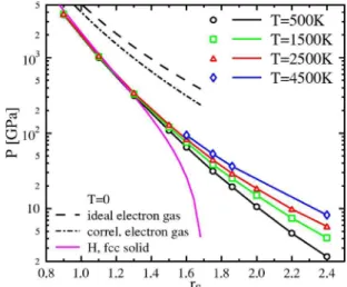
Figure1 provides a summary of our hydrogen EOS cal-culations using DFT-MD. Four different pressure isochores are shown. At low density共rs= 2.4兲, the pressure increases monotonically with temperature as the character of the fluid changes smoothly from molecular to atomic. At this density, the transition is slow enough with temperature so that the drop in the pressure when molecules break共the interactions become less repulsive兲 is compensated by the increase of the kinetic contribution to the pressure.

At higher density共rs⬍ 2兲, the dissociation of molecules takes place more rapidly with increasing temperature and leads to a region of 兩⳵_P/⳵_{T兩V⬍ 0. At sufficiently high}

den-sity, this effect dominates over the pressure increase that re-sults from the ideal kinetic term. Furthermore, the condition 兩⳵P/⳵T兩V⬍ 0 implies a negative thermal expansivity 兩⳵_V/⳵_T兩_{P⬍ 0, while the fluid maintains hydrostatic stability}

given by 兩⳵_P/⳵_{V兩T⬎ 0.}

While earlier CP-MD calculations32_{showed a} discontinu-ous drop in pressure as a function of temperature in the re-gion of dissociation, our BO-MD results in Fig.1 predict a smooth curve with a region of negative slope. This implies

that the dissociation occurs gradually with temperature. The difference between CP-MD and BO-MD was pointed out first by Caspersen et al.,44who carefully analyzed the nature of the dissociation transition using both methods. Small de-viations from the electronic ground-state wave function in CP-MD tend to favor charge delocalization and lead to an artificial enhancement of the dissociation of molecules. These effects are only important in the region of dissociation, and good agreement of BO-MD and previous CP-MD results32_{is found elsewhere.}

By exhibiting a region with 兩⳵P/⳵T兩V⬍ 0, fluid hydrogen shares some properties with typical solids, where a new crys-tal structure with more efficient packing appears and the pressure is lowered at fixed volume. In solid hydrogen dif-ferent transition pressures to an atomic solid have been pre-dicted, above 300 GPa共Refs.52and53兲 and rs⬇ 1.3. This is consistent with the observed shift of the region of 兩⳵_P/⳵_{T兩V⬍ 0 to lower temperatures, as the density is}

in-creased. It indicates a density effect on dissociation as less and less thermal energy is needed to break up the molecular bonds. At even higher densities than shown here, the bond length is equal or less than the mean particle distance. In this regime the interaction of molecules and atoms becomes too strong and pressure dissociation and ionization occur.

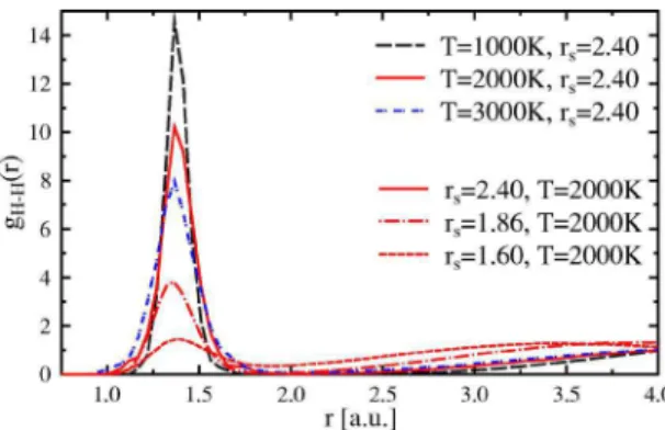
Figure2 shows the dependence of pair correlation func-tions共pure hydrogen at rs= 2.4兲 on the temperature. The first peak at r⬇ 1.40 a.u. indicates the existence of hydrogen mol-ecules. With increasing temperature, the height of the first peak is reduced as molecules dissociate. An analogue behav-ior can be observed by plotting the changes in g共r兲 with density. A strong decrease of the first peak with increasing density, and thus a significant lower fraction of molecules at higher densities is revealed. In addition to the less pro-nounced first maximum, an overall weakening of the short-range order can be observed with increasing temperature.

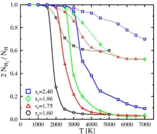
A more quantifiable picture of the described effects can be obtained by plotting the degree of dissociation,

␣=

2NH₂

NH

, 共1兲

as a function of temperature共Fig.3兲. Here NH₂is the average number of hydrogen molecules at the given density and

tem-FIG. 1. 共Color online兲 Pressure-temperature relation for pure hydrogen along various isochores in DFT-MD共this work, different symbols兲 and according to Saumon and Chabrier 共SC, different thick lines兲 共Refs.7and8兲. The isochore of SC for rs= 1.60 lies out

of the range of the P axis. The curves of DFT-MD and SC for r_s = 2.40 agree. The statistical uncertainties in the DFT-MD averages are of the order of the symbols.

FIG. 2. 共Color online兲 Pair correlation functions g共r兲 for pure hydrogen at different temperatures共color coded兲 and different den-sities: solid, dash-dotted, and dashed lines, respectively: r_s = 1.6共0.66 g cm−3_{兲, r}

s= 1.86共0.42 g cm−3兲, and rs

perature conditions. NHis the total number of hydrogen nu-clei irrespectively of the dissociation state.

At higher density, fewer molecules are present at the same temperature as a result of pressure dissociation. While the dissociation proceeds gradually with temperature at low den-sity, the curves for rs艋 1.75 show a rapid drop around 2500 K, which is related to the 兩⳵_P/⳵_{T兩V⬍ 0 region.}

The dissociation degree and the binary distribution func-tion are nevertheless not sufficient to draw a complete pic-ture of the strucpic-ture and dynamics in fluid hydrogen. The lifetime of the molecules must also be taken into account. Figure3shows that at rs= 1.75, for example, even though on average more than 50% of the protons are found in paired states, the lifetime of these pairs is short共less than two H2 vibrations on average兲; there is a continuous formation and destruction of pairs of hydrogen atoms. It is therefore impre-cise to classify the fluid as either molecular-atomic or pure atomic as there is no unique criterion for a molecule. How-ever, the results for the EOS obtained by our simulations do not depend on the number of molecules or atoms but only on temperature and density.

In addition, changes in the electronic structure are of in-terest which take place in the same parameter region as the dissociation of hydrogen molecules. As the system becomes denser or the temperature is raised共still T Ⰶ TF兲, the interac-tions between the molecules in the fluid become stronger and the formerly well-bound electrons become delocalized. This is associated with a strong increase in the electrical conduc-tivity and is usually referred to as metallization.54_{The effect} can be seen in the electronic DOS—namely, the band gap—as shown in Fig.4. We calculated the Kohn-Sham ei-genvalues in the GGA for several snapshots and estimated the band gap in fluid hydrogen along the MD trajectory. For

r_s= 1.6, a closing of the band gap can be observed around

T= 2000 K. This means that a metalliclike state may have been formed. Furthermore, as indicated by the red lines in

Fig.4, the degree of dissociation incorporating lifetime ef-fects decreases strongly around the same temperature. To dis-tinguish this degree of dissociation we do not consider pro-ton pairs with less than 10 H2 vibrations 共t = 10⫻ 7.6 fs兲 as being molecules. The closing of the band gap and dissocia-tion of hydrogen molecules happen at the same time.

It is well known that the GGA underestimates the band gap. More sophisticated calculations55_{共for a H}

2solid兲 give a band gap of⬃0.6 Ha at T = 300 K. The value we obtain is 4 times smaller. Hood and Galli56 _{compared values obtained} with DFT共GGA兲 to QMC gaps for liquid deuterium. For T = 3000 K and rs= 1.6, they found the QMC gap twice as large as the DFT gap. The actual temperature of metalliza-tion is thus somewhat higher. To improve the descripmetalliza-tion of the electronic properties of the fluid, one needs to use a more accurate method than DFT-GGA, which is beyond the scope of this article. Still, it is worth noting that we find a continu-ous transition from an insulating to a conducting state, as determined by the closing of the gap. We do not observe molecules in the conducting phase as found by Weir et al.54 or Johnson and Ashcroft.38

While there is a general agreement about dissociation, ionic, and electronic structural changes throughout various papers, this agreement is only qualitative. As can be seen in Fig.1, different methods give very different results for the EOS of dense fluid hydrogen. Whereas for the lowest density shown in Fig. 1 the agreement between the free energy model of Saumon and Chabrier7,8and our results is reason-able, deviations up to 20% 共at rs= 1.86兲 and even 24% 共at

rs= 1.75 and above兲 can be found for higher densities. The free energy model overestimates the pressure considerably. The degrees of dissociation calculated with the free energy method show a significantly higher fraction of molecules than we find in our simulations. However, even a linear ex-trapolation of our pressure results of the molecular phase to higher temperatures共a linear scaling very similar to the one at rs= 2.4 is assumed兲 only reduces the discrepancy with the result of Saumon and Chabrier but cannot eliminate the dif-ference completely. Deviations of this order may signify completely different physics inside giant gas planets, and it is of great importance to discuss the discrepancies.

FIG. 3.共Color online兲 Dissociation degree of the hydrogen mol-ecules in pure hydrogen. The dissociation degree obtained by sim-ply counting all pairs of hydrogen atoms with distance shorter than

rcut= 1.8 a.u.. is plotted with dotted lines. Solid lines take into

ac-count the lifetime of these pairs as well共ten H2vibrations at least to

be counted as molecule兲.

FIG. 4.共Color online兲 Band gap calculated in the GGA for fluid hydrogen and hydrogen-helium mixture 共blue curves兲 as well as dissociation degree for the two systems共red curves兲. The density corresponds to rs= 1.6. The dissociation degree is determined by

Comparisons with different first-principles calculations can help resolve this issue, as agreement between different independent ab initio methods would be a strong indication for correct results. Figure5 provides such a comparison. In addition to our results, PIMC data,29 _{wave packet molecular} dynamics 共WPMD兲 results,58,61,62 _{and older DFT-MD} points59are shown. Furthermore, the isochores of two differ-ent models in the chemical picture are added: fluid varia-tional theory57 _{共FVT兲 as well as the linear mixing 共LM兲} model.14_{They start from a mixture of atoms and molecules} and their共Lennard-Jones-type兲 interactions to minimize the free energy with respect to the fraction of the constituents. The isochore provided by WPMD deviates from the other ones by more than a factor of 2 at lower temperatures and by 25% at the highest temperatures shown here. PIMC is not a ground-state method and is more capable of determining the EOS at higher temperatures. Information about fluid hydro-gen or even about dissociation of hydrohydro-gen molecules cannot be obtained. For higher temperatures, PIMC results lie be-tween DFT-MD and FVT data. Better agreement is achieved between the two DFT-MD methods, FVT and LM. In the region with temperatures less than 10 000 K some features of the curves are still different. The first-principles simula-tions show a region with a reduced or even slightly negative slope 共smooth transition from a purely molecular to an atomic fluid兲 around 5000 K. Such a behavior is absent in the FVT model. The LM method, on the other hand, shows a similar feature but on a much wider temperature range. Thus, there is no unique picture of the EOS of dense fluid hydro-gen. Deviations between the results of different first-principles methods are related to the treatment of the elec-trons. Inconsistencies between the chemical picture, as a basis for FVT and LM, and the physical picture, as a foun-dation of DFT-MD or PIMC, contribute to the nonunique description. However that may be, DFT-MD provides

repro-ducible results 共the two DFT-MD studies were performed with different codes兲 and FVT seems to be reliable in the molecular fluid phase.

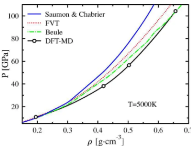
Last, we consider more closely the intermediate density range at a temperature typical for the interior of Jupiter. Fig-ure 6 shows such an isotherm for T = 5000 K. Our result gives the lowest pressure. Saumon and Chabrier’s EOS pre-dicts a pressure up to 20% higher as stated above. The blue curve, as well as the green one, shows a plasma phase tran-sition共PPT兲. According to Saumon and Chabrier the PPT is expected at a density of approximately ␳= 1 g cm−3 共P = 200 GPa兲. The FVT results with13_{or without}10_extension to ionized plasmas give an isotherm right between the two above mentioned results. These methods predict a PPT at slightly smaller density of ␳= 0.8 g cm−3 _{and P = 100 GPa兲.} At both densities, neither we nor Weir et al.54_{have evidence} for such a PPT. Instead, a continuous transition from a mo-lecular to an atomic state takes place at lower temperatures. It is nevertheless remarkable that the inclusion of ionization reduces the pressure and gives better agreement. From our simulation we have no information about possible interme-diate ionized states of hydrogen.

B. Hydrogen-helium mixtures

So far we have studied pure hydrogen under giant gas planet conditions. A further degree of freedom is added if one considers a mixture of hydrogen and helium. Helium, even in small fractions, changes the EOS significantly. He-lium has an influence on the formation and dissociation of hydrogen molecules, and it changes the ionic structure of the liquid as well as the electronic properties. The transition from a molecular state into an atomic state may be displaced or its character changed. Further, hydrogen and helium have been predicted to phase separate in giant planet interiors.6,63,64

Models in the chemical picture use the linear mixing rule to add hydrogen and helium portions to the EOS.65 Contri-butions from the entropy of mixing are ignored, and all the

FIG. 5.共Color online兲 Pressure-temperature relation for a single isochore of hydrogen with different methods for r_s= 2. Our DFT-MD results are shown as blue circles. FVT by Juranek and Redmer共Ref.57兲 共solid black line兲, PIMC by Militzer and Ceperley 共Ref.29兲 共dotted line, triangles兲, WPMD by Knaup et al. 共Ref.58兲 共dashed line, squares兲, DFT-MD by Collins et al. 共Ref.59兲 共dashed, diamonds兲, and LM Ross 共Ref.14兲 共long-short dashed兲. The black dot indicates the pressure of a H₂solid at T = 300 K共Ref.60兲. The statistical uncertainties in the DFT-MD averages are of the order of the symbols.

FIG. 6. 共Color online兲 The 5000-K pressure isotherm of hydro-gen computed with various methods: this works DFT-MD共black with circles兲, FVT 共red兲 共Ref.10兲, Beule 共FVT+ ionization, green兲 共Ref. 13兲, and Saumon and Chabrier 共blue solid兲 共Ref. 8兲. HNC-MAL共Ref.12兲 gives similar results as FVT.

interactions between the two subsystems are left out. First-principles calculations include all these effects since a mix-ture of the two fluids can be simulated directly. The demix-ing line was calculated by classical Monte Carlo simulations,66 _{by ground-state DFT calculations,}16 _{and by} Car Parinello MD.43

Here, we primarily present results for a hydrogen-helium mixture at a mixing ratio of x = 0.5. The mixing ratio is de-fined as

x= 2NHe 2NHe+ NH

, 共2兲

where NHand NHeare the number of hydrogen and helium nuclei per unit volume. This definition weights the species according to the number of electrons that they contribute to the system. The corresponding Wigner-Seitz radius is com-puted from the total number of electrons. For many simula-tions, a mixing ratio of x = 0.5 was chosen so that large in-teraction effects between the two species could be observed. Figure7shows the pressure for a number of isotherms for a hydrogen-helium mixture. The maximum density shown here corresponds approximately to conditions in the center of Jupiter共rs= 0.9,␳= 3.6 g cm−3兲. It is demonstrated that tem-perature is not important for higher densities since all the isotherms merge into the one with the lowest temperature. At the highest density shown here the temperature contribution of the ions to the pressure is approximately 5%. The ions are strongly coupled, and their interaction contribution to the EOS is of the order of 30%. The rest of the deviation from the ideal degenerate system is given by nonidealities in the electron gas and interactions between electrons and ions. For even higher densities the electronic contributions will be-come even more important since they rise with density as

n5/3_{and thus faster than any other contribution.}

The role of helium for the EOS of the mixture can be studied in Fig.8. The pressure is slightly lowered over the whole temperature range, but more important is the fact that

the region with negative兩⳵P/⳵T兩V has vanished共for x = 0.5兲. The additional curve for Jupiter’s hydrogen-helium mixing ratio共x = 0.14兲 shows an intermediate region with a negative slope but the size of the drop in pressure is reduced signifi-cantly. More helium in the mixture also means a shift of the negative slope to higher temperatures. At high temperature, where the hydrogen molecules are dissociated, the pressure depends very little on the helium concentration. Only in the molecular regime does the pressure reduce when hydrogen molecules are replaced by helium atoms because the latter are much smaller than the former.

These two different regions can clearly be assigned to different dissociation regimes 共see Fig. 9兲. The transition from a molecular phase to an atomic phase, while still smooth, takes place at lower temperature and over a shorter range of temperature in hydrogen than in the mixture. This relatively rapid change in the microstructure of the fluid is

FIG. 7. 共Color online兲 Pressure isotherms of a mixture of hy-drogen and helium共x = 0.5兲 for different temperatures. High-density limiting results for hydrogen and an electron gas are shown additionally.

FIG. 8. 共Color online兲 Pressure isochores for a mixture of hy-drogen and helium共x = 0.5, solid lines兲 and for pure hydrogen 共dot-ted lines兲 at two different densities. For rs= 160 an additional curve

for Jupiter’s helium ratio共x = 0.14兲 was added 共black dashed line兲.

FIG. 9. 共Color online兲 Comparison of dissociation degrees 共incorporating life time effects兲 in pure hydrogen and in a hydrogen-helium mixture共x = 0.5兲. The solid lines are nonlinear fits to the data points for the hydrogen-helium mixture共x = 0.5兲.

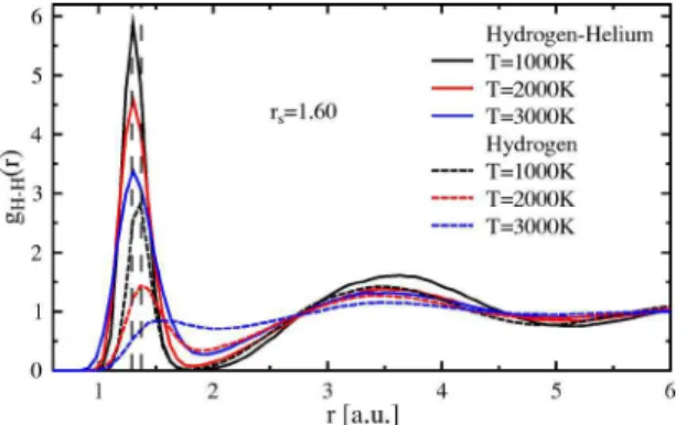
the reason for the drop in the pressure. The vanishing of the molecules in hydrogen and their extended existence in the mixture can be confirmed with the help of pair correlation functions in Fig.10. The molecular peak 共first peak兲 drops considerably faster in pure hydrogen. This behavior and the higher peak in the mixture give clear evidence for molecules at the highest temperatures shown here. If we take the posi-tion of the first maximum as a measure for the mean bond length of the hydrogen molecule, we obtain a value of具d典 = 1.37a0 for pure hydrogen. In the mixture 共with ratio of x = 0.5兲 this value changes to 具d典 = 1.29a0which means a short-ening of the bond by 6%. The same can be obtained by means of nearest-neighbor distributions as in Fig. 11. The first-neighbor distribution considers the nearest neighbor only and effects of particles farther away are removed from the curve. Bond lengths obtained from Fig. 11 are slightly larger. In addition, a shift of the bond length in hydrogen from 1000 to 2000 K is revealed. The reduction of the bond length of 6% is confirmed. The latter value is in rather good agreement with data by Pfaffenzeller et al.43The same

con-clusion is derived when comparing pair correlation functions for pure hydrogen and hydrogen-helium mixtures at constant pressure instead of at constant electronic density.

Figure9describes the role of the共electronic兲 density dur-ing the process of dissociation. Helium stabilizes the mol-ecules. This is due to the higher charge of Z = 2 of the helium nuclei. The intramolecular bonds depend strongly on the electronic behavior and the space available. If electronic wave functions between different molecules start to overlap—in other words, when Fermi statistics becomes im-portant for the electrons of the system as a whole and when the distances between the particles become so small that in-teractions between the molecules are no longer weak—the electrons are forced to delocalize to obey the Pauli exclusion principle and bonding becomes impossible. Helium under giant gas planet conditions, in atomic form, binds two elec-trons closely. The rest of the hydrogen atoms and elecelec-trons are affected less by density and temperature and the mol-ecules remain stable over a wider range. The helium influ-ence is thus in two parts. First, its stronger Coulomb attrac-tion binds electrons. Second共as a consequence兲, it influences the many particle states of the electrons.

A phase diagram for molecular and atomic hydrogen and a hydrogen-helium mixture is provided in Fig.12. Here, pa-rameter regions for purely molecular and purely atomic as well as intermediate phases are shown. The diagram shows the increasing differences between hydrogen and the mixture with increasing pressure 共density兲 and the huge differences 共especially at high pressure兲 in the rate of the transition from a molecular to an atomic state. The transition region 共from 95% to 5%兲 has nearly the same size for small pressures in pure hydrogen and in the mixture. At the other end of the pressure scale, hydrogen changes from molecular to atomic over only 1500 K. In the mixture the changes are more mod-erate. At the pressures considered here, pressure dissociation is suppressed since the slope of the lines with constant dis-sociation degree is small for higher pressures. A good zeroth approximation for the behavior of the mixture is given by taking into account the hydrogen density only for the

disso-FIG. 10.共Color online兲 Pair correlation functions for hydrogen 共dashed lines兲 and a hydrogen-helium mixture 共solid lines兲 at dif-ferent temperatures. The order of the curves from top to bottom is the same as in the legend. The vertical thin dashed lines indicate the location of the first peak for hydrogen and the hydrogen-helium mixture, respectively.

FIG. 11. 共Color online兲 First-neighbor distribution for hydrogen 共dashed lines兲 and a hydrogen-helium mixture 共solid lines兲 at dif-ferent temperatures. The order of the curves from top to bottom is the same as in the legend. The vertical thin dashed lines indicate the location of the peak for hydrogen and the hydrogen-helium mixture, respectively.

FIG. 12.共Color online兲 Temperature-pressure plane showing es-timated lines of constant dissociation degree in pure hydrogen and in a hydrogen-helium mixture共x = 0.5兲. The percentages give the fraction of hydrogen atoms bound in molecules.

ciation process. In this way, rs= 1.6 for a 50% mixture of hydrogen and helium would correspond to rs= 2.02 in pure hydrogen. This estimate works quite well for the 5% line, for instance.

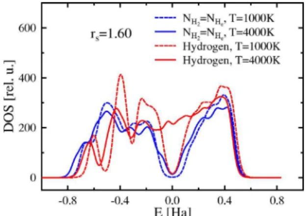
Band structure and electronic density of states are affected also by helium. The inner regions of Jupiter are believed to be made of helium-rich metallic hydrogen.4The conditions under which the mixture becomes metallic strongly depends on the amount of helium. A comparison of the共GGA兲 band gaps in pure hydrogen and a hydrogen-helium mixture 共x = 0.5兲 is shown in Fig. 4. And while the band gap in pure hydrogen goes to zero at relatively low temperatures, the gap in the mixture remains open over the whole temperature re-gion shown. This can be traced back to the charge of the helium nucleus which shifts part of the Kohn-Sham eigen-values to lower energies and thus increases the gap. The change in the electronic DOS from a helium system to a mixture to a pure hydrogen system is shown in Fig.13. The black peak indicates atoms in fluid helium. The red curve shows mainly molecules in hydrogen, and there are peaks resulting from intermolecular interaction, too. The blue curve for the mixture is a superposition of the ones for pure systems—namely, a helium peak to the left and a hydrogen molecule peak on the right-hand side. The bands on the right-hand side are empty since the curves are normalized so that the Fermi energy is at 0 Ha. The position of the edges of the bands at positive and negative energy strongly depends on the amount of helium in the fluid, and therefore the width of the band gap depends on the helium amount.

The dependence of the DOS on temperature is demon-strated in Fig.14. We observe a similar effect as Scandolo did34although the transition from a mainly molecular liquid to an atomic fluid is smooth in our calculations. Due to the larger initial band gap in the hydrogen-helium mixture and due to the effect of the helium described above, the band gap for this system remains, even at the highest temperature shown. Conversely, the gap in the pure system has com-pletely closed at T = 4000 K.

C. Thermodynamic properties of mixtures

We will test the validity of a common approximation used in determining EOS of mixtures. Most of the effort has been put into the determination of the EOS of pure systems. By ignoring the exact nature of the interaction between the pure phases, one can construct the EOS of any mixture of the original phases with the help of the LM approximation

YLM共x兲 = 共1 − x兲YH+ xYHe, 共3兲 with x according to Eq. 共2兲 being the fraction of helium in the mixture and Y being a thermodynamic variable such as volume, pressure, or internal energy. For the free energy, an additional term describing the entropy of mixing must be included.14 Linear mixing may be performed at constant chemical potential, at constant volume, or at constant pres-sure. For calculations of the internal structure of giant gas planets, mixing under constant pressure is the most impor-tant. In all cases, the deviation from LM can be calculated as ⌬Ymix共x兲 = Y共x兲 − YLM共x兲, 共4兲 where Y共x兲 is the value obtained by DFT-MD for mixing fraction x and YLMis the LM value computed from indepen-dent simulation results for pure hydrogen and pure helium33 that we performed.

In this way it is assumed that the potential between par-ticles of two different species can be written as an arithmetic average over the interactions in the pure systems.14This of course works for weak correlations only. The advantage is that one does not need to know exactly the interaction be-tween, e.g., hydrogen and helium. This would be necessary for models in the chemical picture. Therefore, this approxi-mation is used mainly by chemical models for the descrip-tion of hydrogen-helium mixtures7,8,13,57_{or even mixtures of} atoms and molecules of hydrogen.14_{The error introduced is} difficult to quantify.

First-principles calculations are able to verify the assump-tions for LM and the validity of the approximation since these methods rely on the more fundamental Coulomb inter-action, do not need to assume different interaction potentials between different species, and can thus simulate mixtures directly. There have been some investigations concerning the

FIG. 13.共Color online兲 Electronic density of states for pure fluid hydrogen, pure fluid helium, and for a mixture of hydrogen and helium 共x = 0.5兲 at fixed T = 500 K and rs= 1.86. The pressure is

approximately 30 GPa. Curves shifted to agree at the Fermi energy 共0 Ha兲 which is taken in the middle between the highest occupied and lowest unoccupied molecular orbitals.

FIG. 14.共Color online兲 Electronic density of states for pure fluid hydrogen and for a mixture of hydrogen and helium共x = 0.5兲 as a function of temperature. The pressure is approximately 100 GPa.

validity of LM by classical MC and integral equation tech-niques for classical binary liquids not including molecules.67–70_{In these cases, the deviations from LM found} are of the order of 1% and below.

The first PIMC calculations for hydrogen-helium mixtures found deviations from LM at constant volume of up to 12% for temperatures between 15 000 and 60 000 K and giant gas planet densities共rs= 1.86兲.45This gives reason to expect that linear mixing might give a slightly falsified picture of the EOS of a hydrogen-helium mixture at lower temperatures, too. Again, since the conditions for phase separation depend strongly on small changes in the EOS共and thus from devia-tions from LM兲, it is crucial to investigate LM.71_The advan-tage of first-principles calculations is the correct treatment of the degenerate electrons and bound states, which is missing in the classical simulations.

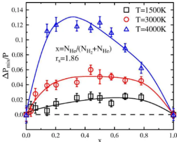
The error introduced due to LM at constant volume 共con-stant electronic density兲 as observed within DFT-MD is plot-ted in Fig. 15. Similar to the findings of other authors,45,70 the error is positive. As expected, the deviation in the pres-sure from the LM value is largest for x = 0.5. Furthermore, increasing temperature causes an increase in the LM error of up to 12% for the highest temperature plotted in Fig.15. The deviation from LM for a Jupiter-like mixing ratio of x ⬇ 0.14 ranges from around zero 共T = 500 K兲 up to 10%. The temperature inside Jupiter for this density is according to Saumon and Chabrier7,8of the order of 5000 K. This means that one can expect a deviation of approximately 10% of the true EOS from the one calculated with LM.

The dependence of the error maximum at x = 0.5 from density and temperature is shown in Fig.16. The curve for the smallest density shown here 共rs= 2.40兲 gives reason to conclude that LM is a good approximation for the pure mo-lecular phase of hydrogen and helium as found at this density over a wide temperature range. With increasing density the deviations from LM start to grow as well and corrections to

the pressure become significant for smaller temperatures. A 5% error is reached around 3000 K for rs= 1.86, around 2500 K for rs= 1.75, and at approximately 1250 K for rs = 1.60. The maximum of ⌬Pmix/ P is located at a slightly higher temperature than the transition from a pure molecular to a mainly atomic phase in pure hydrogen. The linear mix-ing rule transfers the behavior of pure hydrogen in an incor-rect way into the mixture. This causes these deviations of up to approximately 15%. In addition, it is shown that linear mixing is not a good approximation for hydrogen-helium systems containing atoms and molecules. For higher tem-peratures the deviation from linear mixing declines although in the considered range it does not reach values below 5% again.

A similar statement can be made for mixing at constant pressure as shown in Fig.17. The same features as in Fig.16 can be observed. The maximum of the mixing error is shifted

FIG. 15. 共Color online兲 Mixing error in the pressure due to the linear mixing approximation at constant volume for various tem-peratures as a function of the mixing ratio. The electronic density is

rs= 1.86. This corresponds to ̺ = 0.42 g cm−3 for pure H and ̺

= 1.66 g cm−3_{for pure He共pressure between 10 GPa and 40 GPa兲.}

The symbols represent calculated values; the lines were obtained with a polynomial fit of fourth order.

FIG. 16. 共Color online兲 Mixing error in the pressure due to the linear mixing approximation at constant volume for various densi-ties as a function of temperature. The mixing ratio is x = 0.5. The

rs= 2.4 data points suffer from simulation noise, and the curve was

obtained by least-squares fitting a third degree polynomial.

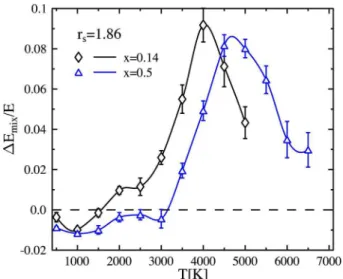
FIG. 17. 共Color online兲 Mixing error in the volume due to the linear mixing approximation at constant pressure for a hydrogen-helium mixture for various densities and two different mixing ratios of x = 0.5 共solid lines兲 and x = 0.14 共dashed line兲 as a function of temperature.

to lower temperatures for higher densities. However, the er-ror in the volume introduced by LM is slightly smaller than the one in the pressure. Comparing curves with different mixing ratios at constant density in Figs. 17 and 18 it is obvious that the maximum in the error is reached at lower temperatures for smaller mixing ratios x. This is in agree-ment with the temperature shift of molecular dissociation as a function of the helium ratio in the system. Less obvious is the actual absolute value for the deviation from linear mix-ing. Whereas the error in the volume never exceeds 5% for a helium fraction as in Jupiter, the energy is much more sen-sitive to deviations from LM with an error of up to 9%.

Figures16–18all show that LM can be considered a good approximation only for systems at low temperatures 共T ⬍ 1000 K兲 and at very high temperatures 共T ⬎ 8000 K兲 for the densities presented here. In the case of liquid hydrogen-helium mixtures, these systems consist of weakly interacting hydrogen molecules and helium atoms共low T兲 or of weakly interacting hydrogen and helium atoms共high T兲. More com-plicated situations where atoms and molecules of hydrogen and helium are involved and interactions between them are non-negligible require a better description than LM since helium has a significant influence on the dissociation degree and the mixture cannot be considered to be a composition of two fluids.

The figures presented here could suggest that LM is a rather good approximation for all of the higher temperatures. This is by no means the case. As stated before, LM works well only for nearly ideal systems. When the temperature becomes too high so that the gas of hydrogen and helium atoms experiences ionization共this can be accomplished by

increasing the density as well兲 and a partially ionized plasma is created, the merely short-range interatomic interactions are replaced by long-range Coulomb forces, and nonideality contributions to the EOS become very important again. In this regime, LM breaks down again, as was demonstrated by Militzer by means of PIMC simulations.45

IV. SUMMARY

We use first-principles DFT-MD simulations to study equilibrium properties of hydrogen and hydrogen-helium mixtures under extreme conditions. The results obtained are relevant for the modeling of giant gas planets and for the principal understanding of the EOS of fluid hydrogen and hydrogen-helium mixtures.

Our results for pure hydrogen show a smooth transition from a molecular to an atomic state which is accompanied by a transition from an insulating to a metalliclike state. In the transition region, we find a negative temperature derivative of the pressure. The results for the hydrogen EOS show de-viations from widely used chemical models共up to 20%兲. In particular, the point of dissociation for the molecules is ob-tained at much lower temperatures than in chemical models. We find satisfying agreement with previous DFT-MD simu-lations only.

In particular, we demonstrate the influence of helium on hydrogen molecules. The presence of helium results in more stable molecules and an altered transition from a molecular to an atomic fluid state. Helium reduces the negative slope of the pressure isochores in the transition region. The bond length of the hydrogen molecules is shortened by 6% for x = 0.5. As a result, the degree of dissociation is lowered and the electronic band gap is increased. The effect of helium is found to be more important for higher densities where the stronger localization of the electrons prevents degeneracy ef-fects for the electrons from becoming dominant.

Our analysis of the mixing properties for a x = 0.5 mixture of hydrogen and helium shows that the corrections to the linear mixing approximation are significant. Maximum EOS corrections of 15% were found for mixing at constant vol-ume and 8% for mixing at constant pressure. For Jupiter-like conditions, corrections up to 5% were obtained.

The presented results and forthcoming work should help to clarify long-standing questions concerning the formation process of giant gas planets, help restrict the core size of Jupiter, and allow one to make predictions for the hydrogen-helium phase separation.

ACKNOWLEDGMENTS

Fruitful discussions with B. Hubbard are acknowledged. This material is based upon work supported by NASA under Grant No. NNG05GH29G, by the Carnegie Institution of Canada, and by the NSF under Grant No. 0507321. I.T. and S.A.B. acknowledge support by the NSERC of Canada.

FIG. 18. 共Color online兲 Mixing error in the energy due to the linear mixing approximation at constant pressure as a function of the temperature for hydrogen-helium mixtures at a density of rs

10_{H. Juranek, R. Redmer, and Y. Rosenfeld, J. Chem. Phys. 117,}

1768共2002兲.

11_{H. Juranek, V. Schwarz, and R. Redmer, J. Phys. A 36, 6181}

共2003兲.

12_{V. Bezkrovniy, M. Schlanges, D. Kremp, and W.-D. Kraeft, Phys.}

Rev. E 69, 061204共2004兲.

13_{D. Beule, W. Ebeling, A. Förster, H. Juranek, S. Nagel, R.}

Red-mer, and G. Röpke, Phys. Rev. B 59, 14177共1999兲.

14_{M. Ross, Phys. Rev. B 58, 669共1998兲.}

15_{W. Kohn and L. J. Sham, Phys. Rev. 140, A1133共1965兲.} 16_{J. E. Klepeis, K. J. Schafer, T. W. Barbee III, and M. Ross,}

Sci-ence 254, 986共1991兲.

17_{I. I. Mazin and R. E. Cohen, Phys. Rev. B 52, R8597共1995兲.} 18_{R. Car and M. Parrinello, Phys. Rev. Lett. 55, 2471共1985兲.} 19_{C. Winisdoerffer, G. Chabrier, and G. Zèrah, Phys. Rev. E 70,}

026403共2004兲.

20_{J. Kohanoff and J.-P. Hansen, Phys. Rev. E 54, 768共1996兲.} 21_{M. W. C. Dharma-wardana and F. Perrot, Phys. Rev. B 66,}

014110共2002兲.

22_{N. W. C. Dharma-wardana and F. Perrot, Phys. Rev. A 26, 2096}

共1982兲.

23_{H. Xu and J.-P. Hansen, Phys. Rev. E 57, 211共1998兲.}

24_{W. R. Magro, D. M. Ceperley, C. Pierleoni, and B. Bernu, Phys.}

Rev. Lett. 76, 1240共1996兲.

25_{C. Pierleoni, D. M. Ceperley, B. Bernu, and W. R. Magro, Phys.}

Rev. Lett. 73, 2145共1994兲.

26_{C. Pierleoni, D. M. Ceperley, and M. Holzmann, Phys. Rev. Lett.}

93, 146402共2004兲.

27_{M. Schlanges, M. Bonitz, and A. Tschttschjan, Contrib. Plasma}

Phys. 35, 109共1995兲.

28_{J. Vorberger, M. Schlanges, and W.-D. Kraeft, Phys. Rev. E 69,}

046407共2004兲.

29_{B. Militzer and D. M. Ceperley, Phys. Rev. Lett. 85, 1890共2000兲.} 30_{B. Militzer, D. M. Ceperley, J. D. Kress, J. D. Johnson, L. A.}

Collins, and S. Mazevet, Phys. Rev. Lett. 87, 275502共2001兲.

31_{V. Bezkrovniy, V. S. Filinov, D. Kremp, M. Bonitz, M.}

Schlanges, W.-D. Kraeft, P. R. Levashov, and V. E. Fortov, Phys. Rev. E 70, 057401共2004兲.

32_{S. A. Bonev, B. Militzer, and G. Galli, Phys. Rev. B 69, 014101}

共2004兲.

33_{B. Militzer, Phys. Rev. Lett. 97, 175501共2006兲.}

34_{S. Scandolo, Proc. Natl. Acad. Sci. U.S.A. 100, 3051共2003兲.} 35_{O. Pfaffenzeller and D. Hohl, J. Phys.: Condens. Matter 9, 11023}

共1997兲.

36_{S. A. Bonev, E. Schwegler, T. Ogitsu, and G. Galli, Nature}

共Lon-don兲 431, 669 共2004兲.

37_{V. Natoli, R. M. Martin, and D. Ceperley, Phys. Rev. Lett. 74,}

1601共1995兲.

http://meetings.aps.org/Meeting/MAR06/Event/42334

45_{B. Militzer, J. Low Temp. Phys. 139, 739共2005兲.}

46_{CPMD, IBM Corp 1990–2006, MPI für Festkörperforschung}

Stut-tgart, 1997–2001.

47_{J. P. Perdew, K. Burke, and M. Ernzerhof, Phys. Rev. Lett. 77,}

3865共1996兲.

48_{N. Troullier and J. L. Martin, Phys. Rev. B 43, 1993共1991兲.} 49_{M. Fuchs and M. Scheffler, Comput. Phys. Commun. 119, 67}

共1999兲.

50_{ABINITgroup, M. Mikami, J. M. Beuken, and X. Gonze, 2003–}

2005.

51_{H. J. Monkhorst and J. D. Pack, Phys. Rev. B 13, 5188共1976兲.} 52_{P. Loubeyre, F. Occelli, and R. LeToullec, Nature共London兲 416,}

613共2002兲.

53_{D. M. Ceperley and B. J. Alder, Phys. Rev. B 36, 2092共1987兲.} 54_{S. T. Weir, A. C. Mitchell, and W. J. Nellis, Phys. Rev. Lett. 76,}

1860共1996兲.

55_{P. Giannozzi and S. Baroni, Phys. Rev. B 30, 7187共1984兲.} 56_{R. J. Hood and G. Galli, J. Chem. Phys. 120, 5691共2004兲.} 57_{H. Juranek and R. Redmer, J. Chem. Phys. 112, 3780共2000兲.} 58_{M. Knaup, P.-G. Reinhard, and C. Toepffer, Contrib. Plasma}

Phys. 39, 57共1999兲.

59_{L. Collins, I Kwon, J. Kress, N. Troullier, and D. Lynch, Phys.}

Rev. E 52, 6202共1995兲.

60_{P. Loubeyre, R. LeToullec, D. Hausermann, M. Hanfland, R. J.}

Hemley, H. K. Mao, and L. W. Finger, Nature共London兲 383, 702共1996兲.

61_{M. Knaup, PhD thesis, University of Erlangen, Germany 2002.} 62_{M. Knaup, P.-G. Reinhardt, C. Toepffer, and G. Zwicknagel,}

Comput. Phys. Commun. 147, 202共2002兲.

63_{D. J. Stevenson and E. E. Salpeter, Astrophys. J., Suppl. 35, 221}

共1977兲.

64_{D. J. Stevenson and E. E. Salpeter, Astrophys. J., Suppl. 35, 239}

共1977兲.

65_{G. Chabrier, D. Saumon, W. B. Hubbard, and J. I. Lunine,}

Astro-phys. J. 391, 817共1992兲.

66_{W. B. Hubbard and H. E. deWitt, Astrophys. J. 290, 388共1985兲.} 67_{S. Ogata, H. Iyetomi, S. Ichimaru, and H. M. Van Horn, Phys.}

Rev. E 48, 1344共1993兲.

68_{H. E. DeWitt, W. Slattery, and G. Chabrier, Physica B 228, 21}

共1996兲.

69_{Y. Rosenfeld, Phys. Rev. E 54, 2827共1996兲.}

70_{H. E. DeWitt and W. Slattery, Contrib. Plasma Phys. 43, 279}

共2003兲.

71_{H. E. DeWitt, Equation of State in Astrophysics, IAU Colloquium}

No. 147 共Cambridge University Press, Cambridge, England, 1994兲.

72_{Phase transition connected with dissociation and ionization of the}