HAL Id: hal-01421011
https://hal.archives-ouvertes.fr/hal-01421011
Submitted on 21 Dec 2016
HAL is a multi-disciplinary open access
archive for the deposit and dissemination of
sci-entific research documents, whether they are
pub-lished or not. The documents may come from
teaching and research institutions in France or
abroad, or from public or private research centers.
L’archive ouverte pluridisciplinaire HAL, est
destinée au dépôt et à la diffusion de documents
scientifiques de niveau recherche, publiés ou non,
émanant des établissements d’enseignement et de
recherche français ou étrangers, des laboratoires
publics ou privés.
A Hybrid Knowledge Discovery Approach for Mining
Predictive Biomarkers in Metabolomic Data
Dhouha Grissa, Blandine Comte, Estelle Pujos-Guillot, Amedeo Napoli
To cite this version:
Dhouha Grissa, Blandine Comte, Estelle Pujos-Guillot, Amedeo Napoli. A Hybrid Knowledge
Dis-covery Approach for Mining Predictive Biomarkers in Metabolomic Data. ECML PKDD, Sep 2016,
Riva del garda, Italy. pp.572 - 587, �10.1007/978-3-319-46128-1_36�. �hal-01421011�
Mining Predictive Biomarkers in Metabolomic
Data
Dhouha Grissa1,3, Blandine Comte1, Estelle Pujos-Guillot2, and Amedeo
Napoli3
1 INRA, UMR1019, UNH-MAPPING, F-63000 Clermont-Ferrand, France 2
INRA, UMR1019, Plateforme d’Exploration du M´etabolisme, F-63000 Clermont-Ferrand, France
3
LORIA, B.P. 239, F-54506 Vandoeuvre-l`es-Nancy, France
Abstract. The analysis of complex and massive biological data issued from metabolomic analytical platforms is a challenge of high importance. The analyzed datasets are constituted of a limited set of individuals and a large set of features where predictive biomarkers of clinical out-comes should be mined. Accordingly, in this paper, we propose a new hybrid knowledge discovery approach for discovering meaningful predic-tive biological patterns. This hybrid approach combines numerical classi-fiers such as SVM, Random Forests (RF) and ANOVA, with a symbolic method, namely Formal Concept Analysis (FCA). The related experi-ments show how we can discover among the best potential predictive biomarkers of metabolic diseases thanks to specific combinations of clas-sifiers mainly involving RF and ANOVA. The visualization of predictive biomarkers is based on heatmaps while FCA is mainly used for visual-ization and interpretation purposes, complementing the computational power of numerical methods.
1
Introduction
The analysis of metabolomic data using data mining methods is one main chal-lenge addressed in this paper. This analysis can be considered as a hard knowl-edge discovery task since data generated by analytical metabolomic platforms, e.g., mass spectrometry (MS), are massive, complex and noisy. In such data, one of the major objectives is to identify, among thousands of features, predictive biomarkers of disease development [11]. More precisely, in the current study, we aim at identifying early predictive biomarkers of T2D, i.e. type 2 diabetes, a few years before occurrence of the disease, in homogeneous populations considered as healthy at the time of analysis. In general, the considered datasets have a limited set of individuals and very large sets of features (or variables) and thus require a specific data processing. In addition, it is desirable that the data analy-sis methods differentiate a two state clinical feature, i.e. healthy vs. not healthy, and contribute to explanations about this difference.
For carrying out the knowledge discovery task, we have to pay attention to the reduction of dimensionality, i.e. feature selection, and to avoid overfitting. Accordingly, we defined a “knowledge discovery workflow” (KD workflow) based on various data mining methods for the discovery of predictive biomarkers from metabolomic data. This KD workflow is based on an original combination of numerical data mining methods to analyze a data table with a large number of numerical features, e.g. molecules or fragments of molecules, and a limited number of individuals (samples), and one binary target variable (having or not the disease at the follow-up, 5 years after the time of analysis). The resulting reduced dataset is then transformed as binary data table that can be used as a context for applying Formal Concept Analysis (FCA [5]) and discovering candi-date biomarkers.
This hybrid knowledge discovery process involve several numerical classifiers including Random Forests (RF) [2], Support vector Machine (SVM) [15], and ANOVA [3]. RF, SVM and ANOVA are used to discover relevant biological patterns which are then organized within a binary table. The numerical clas-sifiers are used for feature selection with the help of filtering methods based on the correlation coefficient and mutual information, for eliminating redun-dant/dependent features, reducing the size of the data table and preparing the application of RF, SVM and ANOVA.
Among the numerous combinations of RF, SVM and ANOVA with the fil-tering methods, we defined ten reference combinations of classifiers (CC) in agreement with the wishes of biologists (especially w.r.t. metabolomic data and usage). Then a comparative study was run to identify the top-k features in com-puting the so-called “top-ranking degree” a feature, i.e. the number of times that a feature is classified among the first features for each CC. Actually, we retained the best ranked features having a top-ranking degree greater or equal to 6. A binary table can then be built, where features are lying in rows and combination of classifiers (CC) are lying in columns. A cell (i, j) in the table is marked with 1 when the feature i has a sufficient top-ranking degree for the CC j. Such a binary table can be in turn considered as a formal context and a starting point for Formal Concept Analysis, and used for the identification of the best features. These last features, which have the best ranking w.r.t. the ten combinations of classifiers, are considered as candidates to be “potential predictive biomarkers”. For experts in metabolomics, it is crucial to compute the ability of the po-tential biomarkers in predicting the disease. This is usually done thanks to ROC analysis [18] which returns a short list of the best features retained as a core set of predictive biomarkers. Based on ROC analysis and FCA, we are able to iden-tify a list of the best combinations of classifiers that provide the best ranking of potential biomarkers. One final objective of this study is to provide a short list of at most 10 biomarkers that can be used in clinical assays, where the simplest combination of metabolites producing an effective predictive outcome must be found. In this way, we can measure the actuality of our knowledge discovery results. This whole process defines an original and hybrid knowledge discovery approach where numerical and symbolic classifiers are combined.
The remainder of this paper is organized as follows. Section 2 provides a description of related works. Section 3 presents the proposed hybrid knowledge discovery approach and explains the analysis of biomarker identification. Sec-tion 4 describes the experiments performed on a real-world metabolomic data set and discusses the results, while Section 5 concludes the paper.
2
State of the art
In [13], authors provide an overview on fundamental aspects of univariate and multivariate analysis related to the analysis of metabolomic data. They make precise the main differences between possible approaches and explain several ex-periments on real and simulated metabolomic data. In this case, the analysis of such data is performed by supervised learning techniques, such as PLS-DA (partial least squares-discriminant analysis), PC-DFA (Principal component-discriminant function analysis), LDA (Linear component-discriminant analysis), RF and SVM.
In [7], authors show that PLS-DA outperforms other approaches in terms of feature selection and classification. In a more detailed study [8], authors compare different variable selection approaches such as LDA, PLS-DA, SVM-Recursive Feature Elimination (RFE), RF (with accuracy and gini), for identifying the best suited method for analyzing metabolomic data and classifying the Gram-positive bacteria Bacillus. They conclude that RF with accuracy and gini and SVM with RFE [9] provide the best results. However, these studies also show that the choice of appropriate algorithms is highly dependent of the dataset characteristics and on the objective of the data mining process.
In the field of biomarker discovery, SVM and RF algorithms proved to be robust for extracting relevant chemical and biological knowledge from complex data, especially in metabolomics [8]. RF is a highly accurate classifier, based on a robust model to outlier detection. One main advantage is its power to deal with overfitting and missing data [1], as well as its ability to handle large datasets.
Finally, in [12], authors discuss recent papers on applying a symbolic classi-fication method such as Formal Concept Analysis in biology and medicine. For example, in [6], authors use a classifier based on FCA to identify combinatorial biomarkers of breast cancer from genes expression values. However, according to literature, no working approach combining supervised and unsupervised data mining techniques was proposed so far for processing metabolomic data. This is precisely the objective of the present paper to fill this gap and to propose an orig-inal combination of numerical and symbolic classifiers for mining metabolomic data.
3
The design of a Hybrid Knowledge Discovery Approach
for Metabolomic Data
In this section, we explain how to design a hybrid knowledge discovery process in agreement with experts in biology and in combining various numerical classifiers,
e.g. RF, SVM, and ANOVA, with a symbolic knowledge discovery method such as FCA, to discover the top-k biological features having a high predictive ability.
3.1 The reduction of dimensionality
Here, the reduction of dimensionality is mainly based on feature selection. This is one of the most important operations that can be carried out, especially con-sidering the data table at hand, with small sets of individuals but very large sets of features. Such an operation requires a careful choice of appropriate feature selection methods [14]. Two main types of approaches can be considered:
– “Filtering” (or filter methods) consists in selecting features using statistical test. Metabolomic data usually contain highly correlated features, leading to some problems when using RF for example [7]. Filter methods allow to select “good features”, such as the “coefficient of correlation” (Cor) or the “mutual information” (MI) measures. Cor and MI can be used to discard highly correlated features for keeping a reasonable number of features to be analyzed.
– The so-called “embedded methods” are searching for an optimal subset of features based on a reference classifier such as RF or SVM [10]. Embedded methods are dependent on the classifier and try to optimize the results of this classifier.
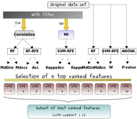
Based on that, we will consider two kinds of classifiers, the first kind using one of the two filters, i.e. correlation coefficient “Cor” and mutual information “MI”, and the other not using any filtering, as this is illustrated by the KD workflow in Figure 1. Filtering based on “Cor” and “MI” eliminates redundant/dependent features, i.e. highly correlated are filtered out and features with MI average values smaller than a given threshold are selected [16]. The result of the filtering is used an an input for the application of the RF and SVM classifiers. Regarding embedded methods, “Recursive Feature Elimination” (RFE), i.e. a backward elimination method proposed in [9] for improving the classification process, is most of the time used for lowering correlation between features when it is still high, either with RF or SVM. Accordingly, we can build three different classifiers, namely RF, RF-RFE and SVM-RFE.
The selection of the top-ranked features can be completed by the use of ac-curacy measures, including “MdGini1”, “MdAcc2”, and “Kappa3”. One general
idea supporting these measures is to permute the values of each feature and then to measure the decrease in accuracy of the classifier.
1 Mean decrease in Gini index (MdGini) provides a measure of the internal structure
of the data.
2 Mean decrease in accuracy (MdAcc) measures the importance/performance of each
feature to the classification.
3 Cohens Kappa (Kappa) is a statistical measure which compares an “observed
In parallel, even if filter methods are generally robust against overfitting, they may still fail to select the best features. For being able to consider this problem, we can apply the classifiers without any filtering, directly working on data. We decided to consider the two classifiers RF and ANOVA alone, and a classifier with an embedded method, namely SVM-RFE. In these last cases, we still can choose accuracy measures such as “MdGini” and “MdAcc”. In addition, we also decided to try the “features weight W”, i.e. the weight magnitude of features, with SVM-RFE, and and the “p-value” with ANOVA, for improving the classification of features and the identification of the features with the highest discriminant ability.
Finally, we design ten different combinations of classifiers (CC) as illustrated in Figure 1. Applying each CC to the original dataset produces a set of “best ranked features” corresponding to the ten datasets called rF Si (for “reduced
Feature Sets”). The ten rF Si include the best ranked features w.r.t. the
corre-sponding CCi.
3.2 Identification of the “top-k best features”
Now, we have at our disposal ten reduced features sets denoted by rF Si of best
ranked features. We will compare these feature datasets and try to discover which are the “top-k features”, i.e. the features which have the best ranking considering all rF Si. This can be likened to a problem of preferences and decision-making,
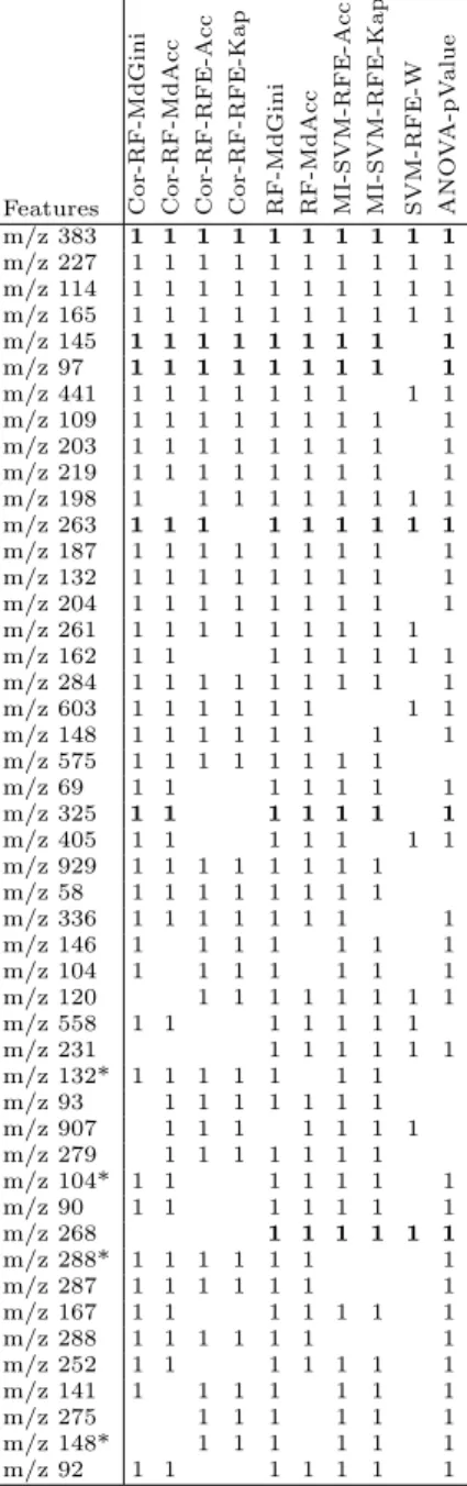
and this is precisely here that symbolic methods can play a major role, and they do. . . A binary table relating features and combinations of classifiers, i.e. f eatures × CC can be designed (see Table 1), where the rows are related to best ranked features and the columns are related to combinations of classifiers (10 CCi).
Each feature has a “top-ranking degree” w.r.t. a given CC. Then, we retain all features which have a top-ranking degree superior or equal to 6, i.e., features belonging to an rF Si (i = 1 . . . 10) and which are top-ranked by at least 6 CC
out of 10.
3.3 Selecting predictive biomarkers (prediction)
For evaluating the predictive power of the best ranked features selected as ex-plained just above, we used the RF classifier again with several configurations, taking the set of the best ranked features as a training set and considering the whole set of available features. In this way, we are able to obtain several different sets of ranked features that can be evaluated thanks to specific evalu-ation measures, namely “sensitivity4”, “specificity5”, “accuracy6”, “precision7”,
“OOB error8” and “misclassification rate9”. Since the number of features to
propose as potential predictive biomarkers should be low and of high biological relevance, we should find the best classifier w.r.t. these evaluation measures.
A second feature selection algorithm based on RF, namely “VarSelRF” [4], can be applied for prediction purpose. VarSelRF is based on a “backward vari-able elimination” for selecting small sets of non-redundant features and provides a reduced set of predictive features. Several trials can be carried out, each pro-ducing a different reduced set of relevant features, until obtaining the lowest OOB error rate.
4 Sensitivity evaluates the efficiency of the classifier in identifying the true positive
instances.
5 Specificity also called true negative rate, measures the proportion of correctly
iden-tified negative instances relative to all real relative ones.
6
Accuracy evaluates the overall performance of the feature selection method, since it measures the ability of the predictive model to correctly classify both positive and negative instances.
7 Precision rates the predictive power of a method, by measuring the proportion of
the true positive instances relative to all the predicted positive ones.
8 A Random Forest classifier returns a measure of error rate based on the out-of-bag
(OOB) cases for each fitted tree.
9 This rate refers to the misclassification rate of the learning model, by estimating the
Then, the results of RF and VarSelRF can be combined, as well as computing the p-values of the selected predictive features using T-tests10. The core set of best features with the smallest p-values and the highest accuracy values is selected to finally obtain a short list of potential predictive biomarkers.
3.4 Visualization and Interpretation
Now we can consider the core set of best ranked features identified in the previ-ous prediction step for visualization and interpretation purposes. Visualization can be carried out using heatmaps, which are currently used in metabolomics and which provide useful insights about the understanding of the metabolomic changes w.r.t. experimental settings and sample groupings. Heatmaps are very useful for patterns recognition in mass spectrometry-based metabolomic domain. They can be used to visualize the results of “biclustering”, e.g. classification w.r.t. the both sets of features and of individuals. Heatmaps represent with different colors the features (or molecules) which predict the set of individuals that are affected or not by the disease. Hotter areas indicate a more intense presence of the feature(s) among individuals. Cooler areas show a lower level of importance.
For completing interpretation of the resulting sets of features and the iden-tification of predictive features, we should find the best classifiers to apply on the metabolomic data at hand. We would like to help the expert to rank the classifiers w.r.t. their ability to detect the best ranked predictive features among a large set of features. A short list of potential predictive biomarkers can be no-ticed in the binary table 1 where they are denoted by bold 1. Then, the related combinations of classifiers can be recommended for reducing dimensionality of metabolomics data and for identifying the best predictive features. Moreover, FCA can be also applied to such a binary table as discussed farther.
4
Experiments
In this section, we discuss the experiments related to our hybrid knowledge discovery approach. Practically, we used a Dell machine running Ubuntu 14.04 LTS, a 3.60 GHZ ×8 CPU and 15, 6 GB RAM. All experiments were performed in the Rstudio software environment (Version 0.98.1103, R 3.1.1).
4.1 The Dataset and its Preparation
The reference dataset is composed of homogeneous individuals considered healthy at the beginning of the study. The binary variable describing the two target classes, i.e. healthy and not healthy, is based on the health status of the same
10T-test or Student T-test is a statistical hypothesis test which can be used to
deter-mine if two sets of data are significantly different from each other. If the p-value is below the threshold chosen for statistical significance (usually the 0.10, the 0.05, or 0.01 level), then the null hypothesis is rejected in favor of the alternative hypothesis.
individuals at another time, actually five years after the initial analysis. Mean-while, some individuals developed the disease. In particular, discriminant fea-tures which enable a good separation between target data classes (healthy vs. not healthy) are not necessarily the best features predicting the disease devel-opment five years later.
More precisely, the dataset to be analyzed is based on a case-control study from the GAZEL French population-based cohort (20000 subjects). This set includes numeric and symbolic data about 111 male subjects (54-64 years old) free of T2D at baseline. Fifty five subjects who developed T2D at the follow-up belong to class ”1” (non healthy or diabetic subjects) while 56 subjects belong to class ”−1” (controls or healthy subjects). 3000 features are generated for each individuals after carrying out mass spectrometry (MS) analysis, resulting in a dataset containing peak intensities (continuous numerical values of these measurements).
The metabolomic database contains thousands of features with a wide in-tensity value range. A data preprocessing step is mandatory for adjusting the importance weights allocated to the features. Thus, before applying any clas-sifier, data are transformed using zero mean normalization and Unit-Variance scaling method. This method removes the average and divides each feature value by its standard deviation. This enables all features to have the same chance to contribute in the classification model when they have an equal unit variance. Finally, the transformed dataset including 1195 features is used as input for all combinations of classifiers.
4.2 The combination of classifiers
Following the KD workflow as introduced in section 3.1 and as depicted in Fig-ure 1, we defined ten different combinations of classifiers (CCi, i = 1 . . . 10) for
feature selections purposes. These ten CCi are detailed hereafter. For example,
“Cor-RF-MdAcc” denotes the sequence of three operations, i.e. the correlation coefficient “Cor” is used on the original dataset for retaining features whose cor-relation value is less than a given threshold, then the classifier Random Forests (RF) is applied, and the final ranking is provided according to the “MdAcc” accuracy measure.
The nine other CCi are named accordingly as (2) “Cor-RF-MdGini”, (3)
“Cor-RF-RFE-Acc”, (4) “Cor-RF-RFE-Kap”, (5) SVM-RFE-Acc”, (6) “MI-SVM-RFE-Kap”, (7) “RF-MdAcc”, (8) “RF-MdGini”, (9) “SVM-RFE-W” and (10) “ANOVA-pValue”.
To work only with important features, we retain the 200 first ranked features from each of the ten CCi, except for the CC “ANOVA-pValue” from which we
only retained 107 features having a “reasonable” p-value (i.e. lower than 0.1). Then, to analyze and interpret the relative importance of each feature, the reduced feature sets rF Si related to each CCi (i = 1 . . . 10) are compared.
Since we are looking for the best ranked features according to the different CCi,
features which are among the best ranked features in at least 6 CCiare selected.
Table 1 whose dimension is 48 × 10, where features are lying in rows and CCi
in columns.
In this binary table, we can identify four features, namely “m/z 383”, “m/z 227”, “m/z 114” and “m/z 165” as the best ranked features for all CCi (i =
1 . . . 10) because they generate a “maximum rectangle full of 1” (the four first rows in Table 1), i.e., they are best ranked in all the 10 CCi. Furthermore, we
can see that some other features are also best ranked by a high number of CCi
such as “m/z 284”, “m/z 204”, “m/z 132”, “m/z 187”, “m/z 219”, “m/z 203”, “m/z 109”, “m/z 97” and “m/z 145”. Moreover, among these 48 best ranked features, 39 are significant w.r.t ANOVA, i.e. the p-value is less that 0.05.
4.3 The Search for Predictive Biomarkers
Here we intend to use two feature selection algorithms, namely “VarSelRF” and “Random Forests”, for prediction purposes. The first algorithm is based on a subset selection method and the second one is based on a feature ranking method as introduced previously.
During the application of “VarSelRF”, it was decided to train the algorithm 100 times and to retain the stable features identified w.r.t. the different replica-tions results. Experiments were performed on the subset of 48 best ranked fea-tures and revealed 5 feafea-tures common to all repeated tests, i.e. “m/z 145”, “m/z 162”, “m/z 263”, “m/z 268” and “m/z 97”, as potential predictive biomarkers. When using the RF classifier, we are highly interested in measuring the im-pact of each feature on the accuracy of classification. Thus, we first split the data into a training set and a test set. Then, we apply the RF classifier on the set of best ranked features including the 48 features using the “MdAcc” measure for ranking. 100 replications of the procedure are performed and the classification with the lowest error is retained. A confusion matrix is generated where a new set of 48 ranked features denoted by RF-MdAcc” is obtained. From “48-RF-MdAcc”, 5 additional sets of features, namely “40-RF”, “30-RF”, “20-RF”, “10-RF” and “5-RF” are built, containing respectively 40, 30, 20, 10 and 5 best ranked features.
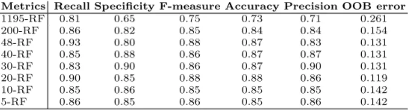
Table 2 summarizes the scores obtained from the six common evaluation metrics, starting from the set of 1195 features, through the set of 200 features (the 200 best ranked features w.r.t. RF with “MdAcc”) until the reduced set of the 5 best ranked features according to RF-MdAcc on the set of 48 best ranked features. The table shows that training RF on the whole data set gives the lowest values. However, reducing data dimensionality to 48 features, better values are obtained. As there is not a set of features which outperforms all the others, the smallest set of the 5 top ranked features, i.e. “m/z 219”, “m/z 268”, “m/z 145”, “m/z 97”, and “m/z 325”, is retained.
In addition, Table 2 shows that only a small fraction of features is discrimi-nant, highlighting the importance of feature selection methods for obtaining the best performances of predictive classifiers. Actually, the RF classifier is able to handle thousands of features, but when applied to the original dataset (1195-RF), it does not achieve a good accuracy (26.1% of OOB error). The set of 48
Features Cor-RF-MdGini Cor-RF-MdAcc Cor-RF-RFE-Acc Cor-RF-RFE-Kap RF-MdGini RF-MdAcc MI-SVM-RFE-Acc MI-SVM-RFE-Kap SVM-RFE-W ANO V A-pV alue m/z 383 1 1 1 1 1 1 1 1 1 1 m/z 227 1 1 1 1 1 1 1 1 1 1 m/z 114 1 1 1 1 1 1 1 1 1 1 m/z 165 1 1 1 1 1 1 1 1 1 1 m/z 145 1 1 1 1 1 1 1 1 1 m/z 97 1 1 1 1 1 1 1 1 1 m/z 441 1 1 1 1 1 1 1 1 1 m/z 109 1 1 1 1 1 1 1 1 1 m/z 203 1 1 1 1 1 1 1 1 1 m/z 219 1 1 1 1 1 1 1 1 1 m/z 198 1 1 1 1 1 1 1 1 1 m/z 263 1 1 1 1 1 1 1 1 1 m/z 187 1 1 1 1 1 1 1 1 1 m/z 132 1 1 1 1 1 1 1 1 1 m/z 204 1 1 1 1 1 1 1 1 1 m/z 261 1 1 1 1 1 1 1 1 1 m/z 162 1 1 1 1 1 1 1 1 m/z 284 1 1 1 1 1 1 1 1 1 m/z 603 1 1 1 1 1 1 1 1 m/z 148 1 1 1 1 1 1 1 1 m/z 575 1 1 1 1 1 1 1 1 m/z 69 1 1 1 1 1 1 1 m/z 325 1 1 1 1 1 1 1 m/z 405 1 1 1 1 1 1 1 m/z 929 1 1 1 1 1 1 1 1 m/z 58 1 1 1 1 1 1 1 1 m/z 336 1 1 1 1 1 1 1 1 m/z 146 1 1 1 1 1 1 1 m/z 104 1 1 1 1 1 1 1 m/z 120 1 1 1 1 1 1 1 1 m/z 558 1 1 1 1 1 1 1 m/z 231 1 1 1 1 1 1 m/z 132* 1 1 1 1 1 1 1 m/z 93 1 1 1 1 1 1 1 m/z 907 1 1 1 1 1 1 1 m/z 279 1 1 1 1 1 1 1 m/z 104* 1 1 1 1 1 1 1 m/z 90 1 1 1 1 1 1 1 m/z 268 1 1 1 1 1 1 m/z 288* 1 1 1 1 1 1 1 m/z 287 1 1 1 1 1 1 1 m/z 167 1 1 1 1 1 1 1 m/z 288 1 1 1 1 1 1 1 m/z 252 1 1 1 1 1 1 1 m/z 141 1 1 1 1 1 1 1 m/z 275 1 1 1 1 1 1 m/z 148* 1 1 1 1 1 1 m/z 92 1 1 1 1 1 1 1
Table 1. The 48 × 10 binary table relating the 48 features which are the best ranked w.r.t. the 10 combinations of classifiers.
Metrics Recall Specificity F-measure Accuracy Precision OOB error 1195-RF 0.81 0.65 0.75 0.73 0.71 0.261 200-RF 0.86 0.82 0.85 0.84 0.84 0.154 48-RF 0.93 0.80 0.88 0.87 0.83 0.131 40-RF 0.85 0.88 0.86 0.87 0.87 0.131 30-RF 0.83 0.90 0.86 0.87 0.90 0.131 20-RF 0.90 0.85 0.88 0.88 0.86 0.119 10-RF 0.85 0.86 0.85 0.85 0.85 0.142 5-RF 0.86 0.85 0.86 0.85 0.86 0.142
Table 2. The values of measures for several sets of features computed with RF and accuracy.
features (48-RF) gives the best value for “Recall” only. The highest values for “precision” and “specificity” are obtained with the set of 30 features i.e. 30-RF. The measures “Accuracy” (which gives an overall estimate of the performance of a classifier) and “F-measure” are better for the set of 20 features. The worst values are measured for the whole data set of 1195 features. This underlines another time the fact that reducing the dimension of the original data table to identify relevant features is essential.
In parallel, using ANOVA, we also retained the 5 best ranked features w.r.t. an ascending order of their their p-value, i.e. “m/z 383”, “m/z 145”, “m/z 97”, “m/z 268”, “m/z 263”. In metabolomics, it is usually interesting to consider features with a small p-value for prediction.
Finally, considering the three features, i.e. “m/z 145”, “m/z 268” and “m/z 97”, which are common to RF and VarSelRF classifiers, plus the top five ANOVA features, we obtain 8 potential predictive features.
4.4 Interpretation of the Potential Biomarkers
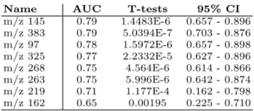
Now we want to show that the 8 selected features are potential predictive biomarkers. This validation is based on the value of AUC and T-tests. Ta-ble 3 shows how the 8 selected features are ranked w.r.t. AUC (univariate ROC curves). This analysis was performed thanks to the ROCCET11tool. If we only
keep features with an AUC higher than or equal to 0.75, and with significantly small T-test values (i.e. smaller than 10E−5), we should exclude two features, namely “m/z 219” and “m/z 162”, leading to a short list of 6 features as potential predictive biomarkers.
In multifactorial diseases such as T2D, a combination of a multiple “weak” multivariate biomarkers instead of a single “strong” individual biomarker often provides the required high levels of discrimination and confidence. Therefore, the performances of the top ranked features (top 8 and top 6) previously obtained are evaluated and compared (see Table 4) using the ROCCET RF tool. The results show that the multivariate top features (top 8 and top 6) are very ac-curate w.r.t. the single features (RF-top5, VarSelRF-top5, ANOVA-top5), with an AUC higher than 0.81. For comparison, we select the six first features having
11
Name AUC T-tests 95% CI m/z 145 0.79 1.4483E-6 0.657 - 0.896 m/z 383 0.79 5.0394E-7 0.703 - 0.876 m/z 97 0.78 1.5972E-6 0.657 - 0.898 m/z 325 0.77 2.2332E-5 0.627 - 0.896 m/z 268 0.75 4.564E-6 0.614 - 0.866 m/z 263 0.75 5.996E-6 0.642 - 0.874 m/z 219 0.71 1.177E-4 0.162 - 0.798 m/z 162 0.65 0.00195 0.225 - 0.710
Table 3. The 8 best AUC ranked features.
Name AUC 95% CI Misclassification (%) RF-top5 0.83 0.749 - 0.923 19.8
VarSelRF-top5 0.841 0.765 - 0.924 22.5 ANOVA-top5 0.826 0.755 - 0.906 20.7 top 8 0.827 0.694 - 0.918 21.6 top 6 0.812 0.714 - 0.903 20.7
Table 4. The 5 predictive classifiers.
an AUC higher than 0.75, and a significant small T-test value for building a multivariate ROC curve. The combination of these single features did not show any improvement in prediction accuracy compared to the multivariate features. Finally, prediction based on the six top ranked features (top 6) shows a misclas-sification rate of 20.7% which is close to the rate of 19.8% obtained by RF-top5.
4.5 Visualization
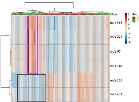
For visualization purposes, we also used “heatmaps” as an easy-to-use inter-active tool for exploring data and results, as heatmaps are commonly used in metabolomics [17]. The rows of the heatmap table represent the features while the columns correspond to the samples or individuals. The color gradient de-notes the normalized abundance of each feature among the samples. Heatmaps can be used to visualize feature classification vs. individual classification. Hotter areas indicate a higher “intensity” of the feature(s) among the individuals.
Figure 2 presents the heatmap corresponding to the 6 × 111 data matrix re-lating the 6 predictive features and the 111 individuals (healthy and not healthy individuals), as a mean to visualize the classification of individuals w.r.t. predic-tive biomarkers. The relationships that can be discovered are very useful for the experts in biology and allow to identify subgroups of individuals who share same metabolite (linked to a feature) levels. For example, from the set of 6 predic-tive features (input), we identify that 4 of them, namely “m/z 383”, “m/z 325”, “m/z 97” and “m/z 145”, which are highly correlated according to Figure 3, characterize a group of individuals with intensity values ranging between 2 and 6 (this group of individuals is described by the highlighted rectangle in Figure 2). Meanwhile both remaining features have very low intensity values (between −4 and 0) for the same group of individuals, but, by contrast, are more present
Fig. 2. A heatmap matrix displaying the predictive power of the 6 best features w.r.t. the 111 individuals. Colors represent the distribution of the data ranging from −6 to 6. From −6 to 0, the features are not representative, while from 0 to 6, the features are more and more representative. The idea is to show the functional relationships among the 6 features and the 111 samples by means of a color-coded matrix elements and adjacent dendrograms. The class −1 represents healthy individuals while class 1 represents not healthy individuals (or patients.
among healthy individuals. These results show the need of combining markers to be able to predict the disease within a whole heterogeneous population.
4.6 The Role of Symbolic KD Methods
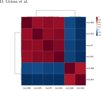
A close examination of the relationships between the best predictive features can contribute to a better understanding of the results Actually, quite strong correlations and associations can be found within the 6 best features. This can help the experts, firstly, in the identification of the structure of metabolites related to predictive features and secondly, in the biological interpretation, as metabolites from a same metabolic pathway should be linked.
Here, it is also time to go back to the role that can be played by symbolic methods in such an hybrid knowledge discovery process. In this way, FCA can be used for information retrieval and visualization purposes, and also to identify the combination of classifiers (CCi) that shows the best behavior. Considering the
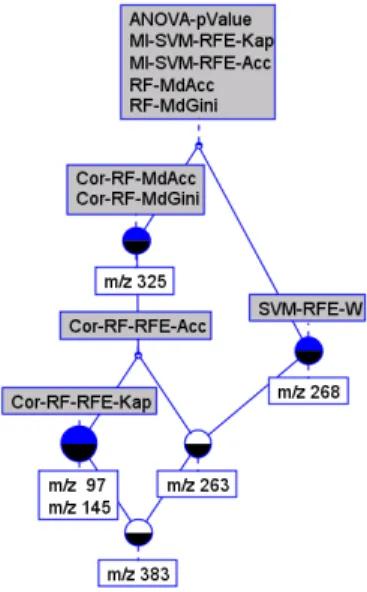
final set of six potential predictive features, we built a binary table corresponding to the part of Table 1 with bold 1. The associated concept lattice can be seen in
Fig. 3. The correlation network based on the 6 best predictive features.
Figure 4, involving 5 combinations of classifiers, namely “ANOVA-pValue”, “MI-SVM-RFE-Kappa”, “MI-SVM-RFE-Acc”, “RF-MdAcc” and “RF-MdGini” and the 6 features. The interpretation of this concept lattice is still under discussion before validation.
In a second time, we consider the 6 best predictive features and their rankings w.r.t the 5 CCi above. Table 5 shows that RF-based techniques and ANOVA
usually give a good ranking to the 6 features by contrast with “MI-SVM-RFE-MdAcc” and “MI-SVM-RFE-Kappa”. For example, “m/z 145” is ranked first ac-cording to “RF-MdAcc”, “RF-MdGini”, second acac-cording to “ANOVA-pValue”, 100th for “MI-SVM-RFE-Acc” and 125th for “MI-SVM-RFE-Kappa”. The fea-ture “m/z 268” is ranked 9th according to “RF-MdAcc”, 6th for “RF-MdGini”, 168th for “MI-SVM-RFE-Acc”, 181th for “MI-SVM-RFE-Kappa”, and 4th for “ANOVA-pValue”. Consequently, the top list combination of classifiers for pre-dictive biomarker identification from metabolomic data is based on RF and ANOVA. However, the choice of appropriate feature selection methods is highly dependent of the dataset characteristics. Moreover, it is also clear that, so far, there is no universal combination of classifiers [8].
Based on these results, one recommendation could be to explore the com-bination of ANOVA and RF-MdGini methods for reducing the dimensional-ity of datasets in metabolomic data, especially when predictive biomarkers are searched.
Fig. 4. The concept lattice of the 6 best predictive features.
Feature RF-MdAcc RF-MdGini MI-SVM-RFE-Acc MI-SVM-RFE-Kappa ANOVA-pValue m/z 145 1 1 100 125 2 m/z 383 3 3 40 39 1 m/z 97 2 2 63 67 3 m/z 325 5 5 38 37 8 m/z 268 9 6 168 181 4 m/z 263 8 7 28 27 5
Table 5. Rankings of the 6 predictive features.
5
Conclusion
In this paper, we presented a new hybrid knowledge discovery process for the identification of relevant predictive biomarkers in metabolomic data. Such data are usually highly correlated and noisy. Accordingly, the reduction of dimen-sionality and feature selection are two tasks of the higher importance. We used classifiers such as Random Forests, SVM and ANOVA, completed by the use of measures for minimizing noise and feature correlations.
This study shows that different combinations of classifiers and measures can be designed and that some of them are better applied to specific datasets, such as metabolomic datasets. Several experiments were performed to assess the predic-tive power of the best ranked features and visualization tools such as heatmaps allowed a deeper interpretation of the results.
In addition, a symbolic knowledge discovery method such as Formal Concept Analysis was used for visualization and interpretation purposes. Such an asso-ciation of numerical and symbolic classifiers is original and should be further
studied. The present paper is a first step in this direction and more extended theoretical studies and experiments remain to be done.
References
1. Biau, G.: Analysis of a Random Forests Model. Journal of Machine Learning Re-search 13(1), 1063–1095 (2012)
2. Breiman, L.: Random Forests. Machine Learning 45(1), 5–32 (2001)
3. Cho, H., Kim, S., Jeong, M., Park, Y., Miller, N., Ziegler, T., Jones, D.: Discovery of metabolite features for the modelling and analysis of high-resolution nmr spectra. International Journal of Data Mining and Bioinformatics 2(2), 176–192 (2008) 4. D´ıaz-Uriarte, R., de Andr´es, S.A.: Gene selection and classification of microarray
data using random forest. BMC Bioinformatics 7(1), 1–13 (2006)
5. Ganter, B., Wille, R.: Formal Concept Analysis - Mathematical Foundations. Springer (1999)
6. Gebert, J., Motameny, S., Faigle, U., Forst, C., Schrader, R.: Identifying Genes of Gene Regulatory Networks Using Formal Concept Analysis. Journal of Computa-tional Biology 2, 185–194 (2008)
7. Gromski, P., Muhamadali, H., Ellis, D., Xu, Y., Correa, E., Turner, M., Goodacre, R.: A Tutorial Review: Metabolomics and Partial Least Squares-Discriminant Analysis–A Marriage of Convenience or a Shotgun Wedding. Analytica Chimica Acta 879, 10–23 (2015)
8. Gromski, P., Xu, Y., Correa, E., Ellis, D., Turner, M., Goodacre, R.: A Compar-ative Investigation of Modern Feature Selection and Classification Approaches for the Analysis of Mass Spectrometry Data. Analytica Chimica Acta 829, 1–8 (2014) 9. Guyon, I., Weston, J., Barnhill, S., Vapnik, V.: Gene Selection for Cancer
Classi-fication Using Support Vector Machines. Machine Learning 46, 389–422 (2002) 10. Lal, T., Chapelle, O., Weston, J., Elisseeff, A.: Feature Extraction: Foundations and
Applications. In: Guyon, I., , Nikravesh, M., Gunn, S., Zadeh, L. (eds.) Embedded Methods, pp. 137–165. Springer (2006)
11. Mamas, M., Dunn, W., Neyses, L., Goodacre, R.: The Role of Metabolites and Metabolomics in Clinically Applicable Biomarkers of Disease. Archive of Toxicol-ogy 85(1), 5–17 (2011)
12. Poelmans, J., Kuznetsov, S., Ignatov, D., Dedene, G.: Formal Concept Analysis in Knowledge Processing: A Survey on Models and Techniques. Expert Systems with Applications 40(16), 6601–6623 (2013)
13. Saccenti, E., Hoefsloot, H., Smilde, A., Westerhuis, J., Hendriks, M.: Reflections on Univariate and Multivariate Analysis of Metabolomics Data. Metabolomics 10(3), 361–374 (2014)
14. Saeys, Y., Inza, I., Larraaga, P.: A Review of Feature Selection Techniques in Bioinformatics. Bioinformatics 23(19), 2507–2517 (2007)
15. Vapnik, V.: Statistical Learning Theory. Wiley-Interscience (1998)
16. Wang, H., Khoshgoftaar, T., Wald, R.: Measuring Stability of Feature Selection Techniques on Real-World Software Datasets. Information Reuse and Integration in Academia and Industry, pp. 113–132. Springer (2013)
17. Wilkinson, L., Friendly, M.: The History of The Cluster Heat Map. The American Statistician pp. 179–184 (2009)
18. Xia, J., Broadhurst, D., Wilson, M., Wishart, D.: Translational Biomarker Dis-covery in Clinical Metabolomics: An Introductory Tutorial. Metabolomics 9(2), 280–99 (2013)