APS/123-QED
Asymmetric source acoustic LWD for the improved formation
shear velocity estimation
Tianrun Chen, Bing Wang, Zhenya Zhu, and Dan Burns
Earth Resources Laboratory, Department of Earth Atmospheric and Planetary Sciences, Massachusetts Institute of Technology, Cambridge, Massachusetts 02139
Abstract
Most acoustic LWD tools generate a single pure borehole mode (e.g., dipole or quadrupole) to estimate the formation shear velocity. We propose an approach where many borehole modes are generated and all the modes are used simultaneously to obtain a better shear estimate. In this approach we find the best fit to the dispersion characteristics of a number of modes, rather than one mode. We propose using an asymmetric source, that is a single source on one side of the tool, together with arrays of receivers distributed azimuthally around the tool to allow different modes to be identified and analyzed. We investigate such an approach using synthetic and laboratory data. The lab data uses a scale-model LWD tool with one active sources transducer mounted on the side of the tool. This source geometry generates monopole, dipole, and quadrupole modes simultaneously. Four sets of receiver arrays, each separated by 90 degrees azimuthally, are used to isolate and analyze each of these modes by adding and subtracting the signals received from different arrays. Based on the dispersion analysis and the method of least square fitting, we find that the by simultaneously using both dipole and quadrupole modes, we can reduce the residual error of the best fit shear velocity. It should be noted that higher order modes (e.g., hexapole, etc) will also be generated by an asymmetric source, and these modes could also be utilized with the appropriate azimuthal receiver configuration.
I. INTRODUCTION
Acoustic LWD tools have been designed with specific applications in mind. Early tools were extensions of wireline sonic logs with sources and receivers located on one side of the rigid tool body. These tools would depend on generating and measuring refracted arrivals along the borehole wall to estimate formation velocities. Later designs, following on the developments in wireline logging, moved towards symmetrically mounted sources on the tool body to generate specific borehole modes such as the dipole or quadrupole in addition to more standard monopole modes. By firing the sources in phase, compressional arrivals could be measured to estimate P wave velocity in the formation. By firing the sources out of phase, higher order modes, such as dipole and quadrupole, would be generated to provide estimates of the formation S wave velocity. Because of the presence of a large diameter rigid tool body, however, the presence of tool modes created complications in most of these cases. These tool modes also interact with the formation modes making interpretation of formation properties more difficult (Rao et al., 1999). In practice the estimation of formation shear velocity from LWD data can be quite challenging because the modes are dispersive and only at the cutoff frequency of the mode is the phase velocity equal to the formation shear velocity. In the case of dipole logging, it is difficult to generate this mode at low enough frequencies to obtain this estimate. The presence of a tool flexural mode that interacts strongly with the formation flexural mode in these frequency ranges further complicates the analysis. Quadrupole logging has the advantage of not having an interfering tool screw mode to deal with, however the dispersion problem remains an issue as does the lower excitation energy of this mode. To address the dispersion problem, Rao and Toksoz (2005) developed a method of estimating the dispersion curves from time series data through the use of a series of narrow bandpass filters combined with time semblance analysis. With such a method it is possible to estimate the shear velocity of the dipole or quadrupole mode by fitting the dispersion curve for some frequency range. With this approach a dispersion correction could be used to estimate the formation shear velocity when the frequency range of the measurements does not include the cut off frequency.
An additional complication exists if the tool is not centered in the borehole or the source transducers are not matched. In these situations pure dipole or quadrupole modes will not be excited as both higher and lower order modes will also be generated. Byun et al. (2004)
and Byun and Toksoz (2006) studied the effects of source mismatch and off-center tools on the modes generated in acoustic LWD. Although the dipole or quadrupole modes could still be isolated by appropriate summation of receivers located around the tool circumference, Stoneley and higher order modes were also present in the time series.
The result of each of these complications is that estimated shear velocities from acoustic LWD data may have significant error. An example of such errors is given in Briggs et al. (2004), where a comparison of shear wave velocity measured by wireline and dipole LWD showed differences averaging 5-7%, with some zones showing differences greater than 10%. In general there was a consistent bias with the LWD values being faster than the wireline values (Briggs et al., 2004). Although these disagreements could, in part, be due to the fact that the wireline data was collected 10 days later than the LWD data allowing some time for alteration and invasion effects to take place, it is more likely that the bias is due to mode impurity in the LWD data and resulting uncertainty in dispersion corrections applied to the measurements.
These observations and previous studies suggest another approach to estimate shear veloc-ity. Rather than focus on generating a single pure borehole mode (e.g., dipole, quadrupole, etc) and estimating the shear velocity from that mode, perhaps we could generate several modes each with sensitivity to the shear velocity and then use all the modes simultaneously to obtain a better shear estimate. In this approach we would be fitting the dispersion char-acteristics of a number of modes, rather than one mode. We propose using an asymmetric source, that is a single source on one side of the tool, together with arrays of receivers dis-tributed azimuthally around the tool to allow different modes to be identified and analyzed. In this paper we investigate such an approach using synthetic and laboratory data. The lab data uses a scale-model LWD tool as described in Zhu et al. (2008) with one active sources transducer mounted on the side of the tool. This source geometry generates monopole, dipole, and quadrupole modes simultaneously. We use four sets of receiver arrays each sep-arated by 90 degrees azimuthally to isolate and analyze each of these modes by adding and subtracting the signals received from different arrays. It should be noted that higher order modes (e.g., hexapole, etc) will also be generated by an asymmetric source, and these modes could also be utilized with the appropriate azimuthal receiver configuration.
II. ACOUSTIC MULTIPOLE MODES EXCITED BY AN ASYMMETRIC SOURCE IN THE BOREHOLE: THEORY REVIEW
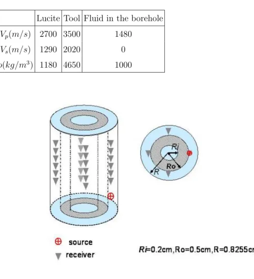
In this section, we will briefly review the method to extract multipole modes from a system with an asymmetric source and four receiver arrays. Fig. 1 shows the geometry of the borehole, positions of the source, receivers and the scaled logging while drilling (LWD) tool used in both the numerical modeling and laboratory measurements. Detailed description of this acoustic tool can be found in Zhu et al (2008). The isotropic slow formation surrounding the borehole is simulated by Lucite (Zhu et al 2008). Other parameters including density, shear and compressional velocities of the tool, fluid in the borehole and Lucite are contained in Table. 1. We made two laboratory measurements where a sinusoid source waveform centered at 50 kHz was used.
The direct acoustic potential excited by an asymmetric source, as shown in Tang and Cheng (2004), is expressed as Φi(r, r0, z, z0, k, ω) = 1 π ∞ X n=0 εn In(f r0)Kn(f r), r > r0 In(f r)Kn(f r0), r < r0
cos(n(θ − θ0))eik(z−z0) (1)
by applying Bessel addition theorem (Watson, 1944), where k is the axial wavenumber,
ω is the angular frequency, r and r0 are the receiver and source distance off the borehole
center respectively, z and z0 are the receiver and source position along z direction, θ0 and θ
are the azimuthal angles of the source and receiver. The radial wavenumber f is equal to
pk2− (ω/c
f)2, where cf is the fluid velocity. Similar to Φi , the scattered potential(Tang
and Cheng, 2004) in the borehole can be written as
Φsca(k, ω) =
∞ X
n=0
DnIn(f r)cos(n(θ − θ0))eik(z−z0), (2)
where Dn can be determined by matching the boundary conditions between the formation
and fluid in the borehole, the fluid in the borehole and the tool as well as the tool and
the inner fluid. The total potential Φtot(k, ω) in the borehole is the sum of the direct and
the scattered potentials. We can calculate the dispersion curve for the multipole modes
by searching the local maximum value of Φtot(k, ω) on the frequency-wavenumber domain.
Fig. 2(a), 2(b) and 2(c) show the dispersion curve of monopole, dipole and quadrupole mode respectively. The monopole mode (Stoneley wave) represented by blue stars does not show much dispersion behavior. The red circles show the dispersion of the P head wave
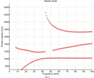
modes whose velocity is almost frequency invariant. The dispersion curve of the dipole mode (flexural wave), as represented by red circles, shows a divergence at both low and high frequencies. This is caused by the different dispersion characteristic between the tool and the dipole modes (Rao et al 2004). The dipole mode only shows strong dispersive behavior at frequencies below 35kHz, while its phase velocity is almost flat at frequencies higher than
40kHz. Fig. 2(d) shows the amplitude of Φtot(k, ω) at frequencies 20k 45k and 75k. The
amplitude of the tool mode is much larger than that of dipole mode at frequencies below 35kHz and vice versa at frequencies higher than 40kHz, which indicates that the dipole mode can be detected at higher frequency range. Fig. 2(c) shows moderate dispersion behavior of the quadrupole mode.
When only an asymmetric source is in the borehole, all modes are simultaneously ex-cited. Since each mode is azimuthally orthogonal to each other, receiver arrays over a range of azimuthal directions are required to resolved each individual mode. With only four
re-ceivers distributed at 0o, 90o, 180o and 270o azimuthal angles, as shown in Fig. 1, we can
approximately resolve the monopole, dipole and quadrupole modes by assuming all higher order modes are negligible compared to them. The total potentials at these four receivers can be expressed as
Φtotr1 (θ = 0) = M + D + Q + ǫ; (3)
Φtotr2 (θ = π/2) = M − Q + ǫ;
Φtotr3 (θ = π) = M − D + Q + ǫ;
Φtotr4 (θ = 3π/2) = M − Q + ǫ,
where the source is put at 0o azimuthal angle without losing generality, M, D and Q are the
total potential of monopole, dipole and quadrupole modes and ǫ is the sum of higher order potential. By adding and subtracting the potentials expressed in Eq. 4, the potentials of the monopole, dipole and quadrupole modes are
Φmono = Φtotr1 + Φtotr2 + Φtotr3 + Φtotr4 , Φdi= Φtotr1 − Φtotr3 ,
Φquadru = Φtotr1 − Φtotr2 + Φtotr3 − Φtotr4 . (4)
We can also resolve hexapole, octupole and higher modes with more receivers symmetrically distributed over the azimuthal direction.
III. NUMERICAL MODELING AND LABORATORY MEASUREMENTS
In this section, we will investigate the acoustic field of the monopole, dipole and quadrupole modes excited by an asymmetric source in a borehole through numerical mod-eling and laboratory measurements. We will show the simulated and measured time traces for these modes, and then perform the time-velocity semblance and frequency-velocity dis-persion analysis on the time traces.
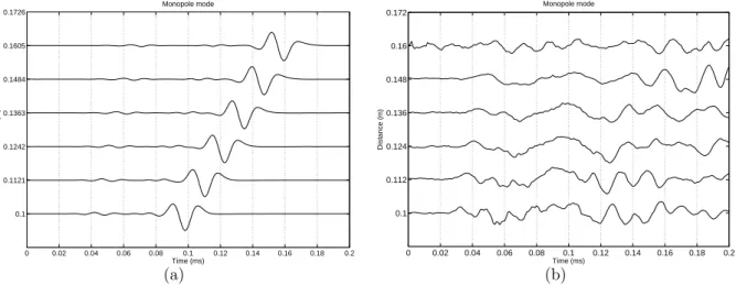
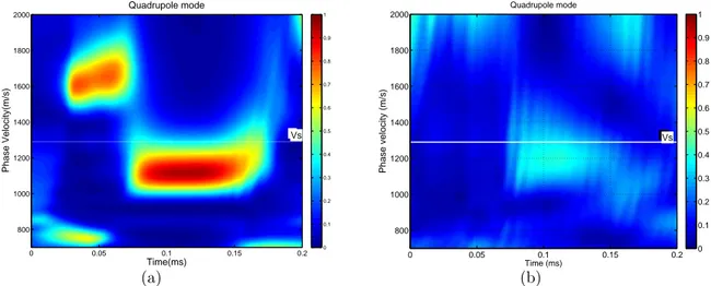
Fig. 3(a), 4(a) and 5(a) show the time traces of modeled monopole, dipole and quadrupole modes respectively, while Fig. 3(b), 4(a) and 5(a) show the measured traces of the same multipole modes. All the measured traces have been averaged over 32 source firings to reduce the noise. From the time traces, we apply a non-dispersive waveform coherence stacking method by Kimball and Marzetta (1986) to calculate the time-velocity semblances. The simulated time semblance of monopole mode shows clear arrivals of formation’s com-pressional waves (P head waves), which are marked by a white line in Fig. 6(a). The Stoneley waves propagate at a speed slightly smaller than 1000m/s. Fig. 6(b) shows the semblance for monopole mode from the laboratory data. The coherence of Stoneley wave arrivals is very small compared to the simulations. This is because that the Stoneley wave may not be effectively excited by the source waveform with 50kHz central frequency. Therefore, we will exclude the monopole mode and only use dipole and quadrupole modes in the formation velocity inversion. Both Figs. 7(a) and 7(b) show strong flexural wave (dipole mode) arrivals in the numerical simulations and the laboratory measurements. In Figs. 8(a) and 8(b), we show the semblance of the quadrupole mode for numerical simulations and laboratory mea-surements. The quadrupole mode propagates with a velocity close to 1200m/s in both the numerical simulations and measurements.
This time semblance analysis gives a quick method for estimating the velocity of the formation and multipole modes. However, it does not capture the dispersion characteristics of the guided waves. For these waves, we use an algorithm from Rama Rao and Nafi Toksoz (2005) to perform the dispersion analysis. This process has the following steps:
(1) Fourier transform the received array time series into frequency domain.
(2) For a given frequency ωl, using a Gaussian window to weight the frequency spectral
over a given frequency interval centered at ωl.
(4) Using the same non-dispersive time semblance analysis by Kimball (1986) on the new
time series to get the phase velocity at frequency ωl.
Fig. 9(a) and 9(b) show the estimated dispersion curve of the monopole mode based on the time traces obtained from simulations and measurements, where the white circles on Fig. 9(a) represent the theoretical calculation shown on Fig. 2(a). The fact that the theoretical and the estimated phase velocities match very well is a good indication of the accuracy of this dispersion analysis algorithm. Due to the inefficient excitation, the coherence of the measured monopole mode is very weak. As a result, we decide to disregard the monopole measurements for the shear velocity estimation.
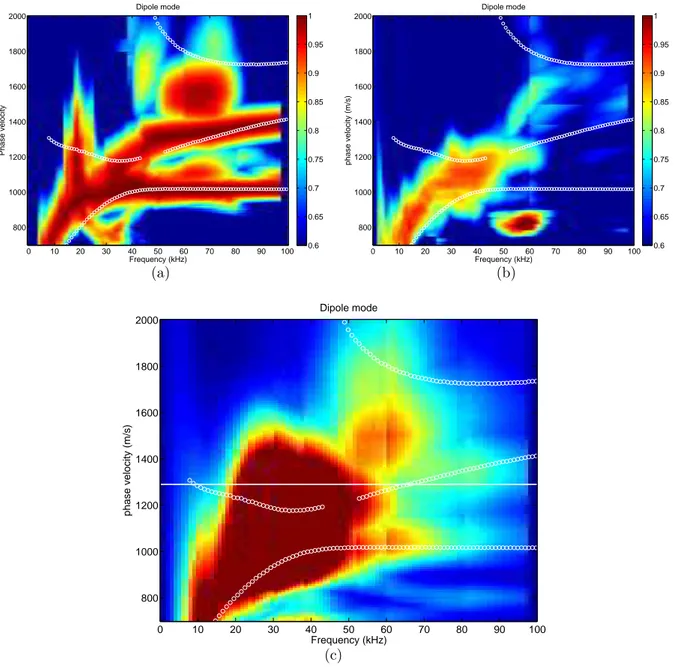
In Fig. 10(a), we find some mismatch of the dispersion curve between the theoretical calculation and estimation for the tool flexural wave. This is due to the insufficient aperture of the receiver arrays over z direction that do not have good enough resolutions over the axial wavenumber k. The interaction between the tool mode, dipole mode and other high order modes leads to higher estimated phase velocities compared to the theoretical ones. At higher frequencies, the match becomes very good for both tool and dipole mode due to relatively weak coupling between them. Fig. 10(b) shows the estimated dispersion curve from the measured time traces. The energy and coherence of tool mode is so strong that it totally masks the dipole mode at frequencies below 40kHz. This makes it is impossible to detect any dipole modes. For frequencies higher than 40kHz, the coherence of the dipole mode is still very weak compared to the tool mode although its amplitude is already larger than that of tool mode, as demonstrated in Fig. 2(d). In order to make use of the coherence and relatively large amplitude of the dipole mode simultaneously, we modify the non-dispersive time semblance analysis by Kimball (1986). Instead of calculating the coherence function defined in Eq. 3.8 of Tang and Cheng (2004)
ρ(s, T ) = RT+Tw T PN m=1Xm(t + s(m − 1)d) 2 dt NPN m=1 RT+Tw T |Xm(t + s(m − 1)d)|2dt (5)
where Xm(t) is the acoustic time signal at the mth receiver in the array of N receivers, with
a receiver spacing d, we use ρ(s, T ) = Z T+Tw T N X m=1 Xm(t + s(m − 1)d) 2 dt (6)
to take into account the effect of amplitude of the time traces. As shown in Fig. 10(c), the dipole mode now can be distinguished from the tool mode and other background “noise” at frequency higher than 40kHz.
Fig. 11(a) shows the dispersion curve for the quadrupole mode including the leaky modes whose velocity are larger than the formation shear velocity. In the laboratory experiment, the energy in the leaky mode is so small that we can not record any signals and the dispersion curve is “cut-off” at the formation shear velocity, as shown in Fig. 11(b). The estimated dispersion curve seems slightly higher than the theoretical one represented by the white circles, as shown in Fig. 11(b). This difference will lead to a higher estimated shear formation velocity.
IV. RESULTS AND DISCUSSION
In this section, we apply the method of least square fitting to estimate the formation shear velocity. For both dipole and quadrupole mode measurements, we apply a band-pass filter between 40kHz to 90kHz to minimize the effects from tools mode.
When estimating the formation shear velocity, we assume that it falls within the range between 1000m/s and 1500m/s. The dispersion curve is then calculated for each assumed
formation shear velocity by searching the local maximum value of Φtot(k, ω). The best
estimation of formation shear velocity is defined to be the one whose sum of squared velocity residuals over a desired frequency range has the least value, where the residual is the phase velocity difference between the laboratory measurements and the modeled ones. There are two independent but equally important parameters that quantify the quality of the estimation: (1) the velocity residual, which indicates the accuracy of the estimation, and (2) the variance of the best estimated value specifying the fluctuations of the estimated value. Ideally, both values should be as small as possible.
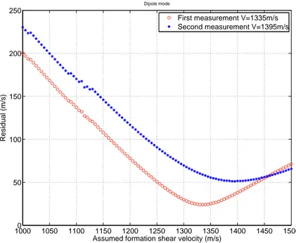
Fig. 12 shows the root of square velocity residuals as a function of the assumed formation shear velocity for dipole mode. It is found that, for the first and second measurements, the best estimation of the formation shear velocities are 1335 m/s and 1395m/s with velocity residual approximate 25m/s and 50m/s respectively. Both measurements have relatively small residuals. The difference (we refer to the variance) between these two estimated results, however, is fairly large and the estimation resolution is not very good especially
for the second measurement. Fig. 13 shows the same plot except for the quadrupole mode. The best estimated formation shear velocity is 1360 m/s and 1365 m/s and the velocity residuals are 96m/s and 40m/s. When compared to the dipole measurements, the quadrupole measurements have much smaller variance of the estimated shear formation velocity, their residuals, however are much bigger than these of dipole mode. When we combine both dipole and quadrupole estimation, as shown in Fig. 14, the best estimated value for these two experiments become 1355m/s and 1365m/s. The velocity residuals are also smaller than the ones solely from quadrupole modes. This may suggest that, by simultaneously using the estimation from both dipole and quadrupole modes, the ambiguity of the formation shear velocity estimation has been reduced without sacrificing much accuracy of the estimation.
V. CONCLUSION AND FUTURE WORK
In this paper, we demonstrate that, by adding and subtracting recorded signals from four-receiver arrays, we are able to extract and separate monopole, dipole and quadrupole modes simultaneously excited by an asymmetric source. Based on the dispersion analysis and the method of least square fitting, we find that the velocity residual based on dipole mode estimation is smaller than that from the quadrupole mode, while the variance of the estimation is larger. By simultaneously using both dipole and quadrupole modes, we combine the advantages of mode resulting in reduced variance while still maintaining a reasonably small residual in the formation velocity estimate. Although we need many more experimental measurements to quantify this variance reduction, these results show that the concept of asymmetric source logging can lead to improved shear velocity estimates. In the future, we plan to build a new scaled LWD tool with more receiver arrays along both the azimuthal and vertical directions so that we can include hexapole or even octupole mode estimation to further improve the accuracy and decrease both ambiguity and residual of the formation velocity.
1 V. Briggs, R. Rao, S. Grandi, D. Burns, and S. Chi, 2004, A comparison of LWD and wireline
dipole sonic data: Annual report of borehole acoustics and logging and reservoir delineation consortia, Massachusetts Institute of Technology.
2 J. Byun, M. N. Tokson, and R. Rao, 2004, Effects of source mismatch on multipole logging:
An-nual report of borehole acoustics and logging and reservoir delineation consortia, Massachusetts Institute of Technology.
3 J. Byun and M. N. Toksoz, 2006, Effects of an off-centered tool on dipole and quadrupole
logging: Geophysics, 71, 91-99
4 C. V. Kimball and T. L. Marzetta, 1986, Semblance processing of borehole acoustic array data:
Geophysics, 49, 274-281
5 B. Nolte and X. J. Huang, 1997, Dispersion analysis of split flexural waves: Annual report of
borehole acoustics and logging and reservoir delineation consortia, Massachusetts Institute of Technology.
6 N. R. Rao, D. R. Burns, and M. N. Toksoz, 1999, Models in LWD Applications: Annual report
of borehole acoustics and logging and reservoir delineation consortia, Massachusetts Institute of Technology.
7 R. Rao. V. N. and M. Nafi. Toksoz, 2005, Dispersive Wave Analysis - Method and
Appli-cations, Annual report of borehole acoustics and logging and reservoir delineation consortia, Massachusetts Institute of Technology.
8 X. M. Tang and A. Cheng, 2004, Quantitative borehole acoustic methods, Elsevier press. 9 G. A. Watson, 1944, A treatise on the theory of bessel functions, Cambridge University press,
second edition.
10 Z. Zhu, M. N. toksoz, R,Rao and D.R.Burns, 2008, Experimental studies of monopole, dipole,
and quadrupole acoustic logging while drilling (LWD) with scaled borehole models: Geophysics, 73, 133-143
Lucite Tool Fluid in the borehole
Vp(m/s) 2700 3500 1480
Vs(m/s) 1290 2020 0
ρ(kg/m3) 1180 4650 1000
0 10 20 30 40 50 60 70 80 90 100 800 1000 1200 1400 1600 1800 2000 2200 2400 2600 2800 3000 Phase velocity (m/s) Frequency (kHz) Monopole mode (a) 0 10 20 30 40 50 60 70 80 90 100 800 1000 1200 1400 1600 1800 2000 2200 2400 Frequency (kHz) Phase velocity (m/s) Dipole mode (b) 0 50 100 150 800 1000 1200 1400 1600 1800 2000 2200 2400 2600 2800 3000 Frequency (kHz) Quadrupole mode Phase velocity (m/s) (c) 800 1000 1200 1400 1600 1800 2000 0 2 4 6 8 10 12 Phase velocity (m/s) Amplitude of Φ tot (k, ω )
Amplitude comparison between tool and dipole mode at 20kHz, 45kHz and 70kHz Frequency = 20kHz Frequency = 45kHz Frequency = 75kHz Tool mode Dipole mode (d)
FIG. 2: Dispersion curves for (a) monopole, (b) dipole and (c) quadrupole modes from theoretical calculations. The amplitude of the total potential field at frequency 20kHz, 45kHz and 75kHz is shown on (d).
0 0.02 0.04 0.06 0.08 0.1 0.12 0.14 0.16 0.18 0.2 0.1 0.1121 0.1242 0.1363 0.1484 0.1605 0.1726 Time (ms) Distance (m) Monopole mode (a) 0 0.02 0.04 0.06 0.08 0.1 0.12 0.14 0.16 0.18 0.2 0.1 0.112 0.124 0.136 0.148 0.16 0.172 Time (ms) Distance (m) Monopole mode (b)
FIG. 3: Time traces of the monopole mode from the (a) numerical modeling and (b) laboratory measurement. 0 0.02 0.04 0.06 0.08 0.1 0.12 0.14 0.16 0.18 0.2 0.1 0.1121 0.1242 0.1363 0.1484 0.1605 0.1726 Time (ms) Distance (m) Dipole mode (a) 0 0.02 0.04 0.06 0.08 0.1 0.12 0.14 0.16 0.18 0.2 0.1 0.112 0.124 0.136 0.148 0.16 0.172 Time (ms) Distance (m) Dipole mode (b)
FIG. 4: Similar to Fig. 3, but for the dipole mode.
0 0.02 0.04 0.06 0.08 0.1 0.12 0.14 0.16 0.18 0.2 0.1 0.1121 0.1242 0.1363 0.1484 0.1605 0.1726 Time (ms) Distance (m) Quadrupole mode (a) 0 0.02 0.04 0.06 0.08 0.1 0.12 0.14 0.16 0.18 0.2 0.1 0.112 0.124 0.136 0.148 0.16 0.172 Time (ms) Distance (m) Quadrupole mode (b)
Phase Velocity(m/s) 0 0.05 0.1 0.15 0.2 1000 1500 2000 2500 3000 3500 Monopole mode Time (ms) 0 0.1 0.2 0.3 0.4 0.5 0.6 0.7 0.8 0.9 Vs Vp (a) Time (ms) Phase velocity (m/s) Monopole mode 0 0.05 0.1 0.15 0.2 1000 1500 2000 2500 3000 3500 0.1 0.2 0.3 0.4 0.5 0.6 0.7 0.8 Vp Vs (b)
FIG. 6: The time-velocity semblance for the (a) modeled and (b) measured monopole mode. The coherence of the measured monopole mode is too weak to be detected.
Time(ms) Phase Velocity(m/s) Dipole Mode 0 0.05 0.1 0.15 0.2 800 1000 1200 1400 1600 1800 2000 0 0.1 0.2 0.3 0.4 0.5 0.6 0.7 0.8 0.9 Vs (a) Time (ms) Phase velocity (m/s) Dipole mode 0 0.05 0.1 0.15 0.2 800 1000 1200 1400 1600 1800 2000 0 0.1 0.2 0.3 0.4 0.5 0.6 0.7 0.8 0.9 1 Vs (b)
FIG. 7: The time-velocity semblance of the dipole mode from (a) the numerical modeling and (b) the laboratory measurement. The flexural wave propagates with a velocity close to 1000m/s in both simulations and measurements.
Time(ms) Phase Velocity(m/s) Quadrupole mode 0 0.05 0.1 0.15 0.2 800 1000 1200 1400 1600 1800 2000 0 0.1 0.2 0.3 0.4 0.5 0.6 0.7 0.8 0.9 1 Vs (a) Time (ms) Phase velocity (m/s) Quadrupole mode 0 0.05 0.1 0.15 0.2 800 1000 1200 1400 1600 1800 2000 0 0.1 0.2 0.3 0.4 0.5 0.6 0.7 0.8 0.9 1 Vs (b)
FIG. 8: The time-velocity semblance of the (a) modeled and (b) measured quadrupole mode.
Monopole mode Frequency (kHz) Phase velocity 0 10 20 30 40 50 60 70 80 90 100 800 1000 1200 1400 1600 1800 2000 0.9 0.91 0.92 0.93 0.94 0.95 0.96 0.97 0.98 0.99 1 (a) Frequency (kHz) Phase velocity (m/s) Monopole mode 0 20 40 60 80 100 800 1000 1200 1400 1600 1800 2000 0.5 0.55 0.6 0.65 0.7 0.75 0.8 0.85 0.9 0.95 1 (b)
FIG. 9: Dispersion curves of the (a) modeled and (b) measured monopole mode estimated from the time traces shown in Fig. 3. The Stoneley wave does not show much dispersive behavior. The excitation of the Stoneley wave in the measurement is very weak, which is also shown in Fig. 6(b).
Dipole mode Frequency (kHz) Phase velocity 0 10 20 30 40 50 60 70 80 90 100 800 1000 1200 1400 1600 1800 2000 0.6 0.65 0.7 0.75 0.8 0.85 0.9 0.95 1 (a) Frequency (kHz) phase velocity (m/s) Dipole mode 0 10 20 30 40 50 60 70 80 90 100 800 1000 1200 1400 1600 1800 2000 0.6 0.65 0.7 0.75 0.8 0.85 0.9 0.95 1 (b) Frequency (kHz) phase velocity (m/s) Dipole mode 0 10 20 30 40 50 60 70 80 90 100 800 1000 1200 1400 1600 1800 2000 (c)
FIG. 10: Dispersion curves of the (a) modeled and (b) measured dipole mode estimated from the time traces shown in Fig. 3. The dispersion curve shown on (c) is based on a weighted coherence function expressed in Eq. 6.
Frequency (kHz) Phase velocity Quadrupole mode 0 10 20 30 40 50 60 70 80 90 100 800 1000 1200 1400 1600 1800 2000 0.4 0.5 0.6 0.7 0.8 0.9 1 (a) Frequency (kHz) Phase velocity (m/s) Quadrupole mode 0 20 40 60 80 100 800 1000 1200 1400 1600 1800 2000 0.4 0.5 0.6 0.7 0.8 0.9 1 (b)
FIG. 11: Dispersion curves of the quadrupole mode from (a) numerical modeling (b) laboratory measurements. All the modes with velocities greater than the formation shear velocity have been “cut-off” due to their weak amplitude in the measurement.
10000 1050 1100 1150 1200 1250 1300 1350 1400 1450 1500 50 100 150 200 250 Dipole mode
Assumed formation shear velocity (m/s)
Residual (m/s)
First measurement V=1335m/s Second measurement V=1395m/s
FIG. 12: Sum of the squared velocity residual versus the assumed formation shear velocity for the dipole mode.
10000 1050 1100 1150 1200 1250 1300 1350 1400 1450 1500 50 100 150 200 250 300 350 Quadrupole
Assumed formation shear velocity (m/s)
Residual (m/s)
1st measurment, Vbest=1360m/s
2nd measurement Vbest=1365m/s
FIG. 13: Similar to Fig. 12, but for the quadrupole mode.
10000 1050 1100 1150 1200 1250 1300 1350 1400 1450 1500 50 100 150 200 250 300 350
Dipole + Quadrupole mode
Velocity(m/s)
Residual(m/s)
1st measurment, Vbest=1355m/s
2nd measurement Vbest=1365m/s
FIG. 14: Sum of the squared velocity residual including both dipole and quadrupole experimental data.