Publisher’s version / Version de l'éditeur:
Vous avez des questions? Nous pouvons vous aider. Pour communiquer directement avec un auteur, consultez la
première page de la revue dans laquelle son article a été publié afin de trouver ses coordonnées. Si vous n’arrivez pas à les repérer, communiquez avec nous à [email protected].
Questions? Contact the NRC Publications Archive team at
[email protected]. If you wish to email the authors directly, please see the first page of the publication for their contact information.
https://publications-cnrc.canada.ca/fra/droits
L’accès à ce site Web et l’utilisation de son contenu sont assujettis aux conditions présentées dans le site LISEZ CES CONDITIONS ATTENTIVEMENT AVANT D’UTILISER CE SITE WEB.
Student Report; no. SR-2009-15, 2009-01-01
READ THESE TERMS AND CONDITIONS CAREFULLY BEFORE USING THIS WEBSITE. https://nrc-publications.canada.ca/eng/copyright
NRC Publications Archive Record / Notice des Archives des publications du CNRC : https://nrc-publications.canada.ca/eng/view/object/?id=75f181b8-beeb-4ab8-9e65-334a0ffff543 https://publications-cnrc.canada.ca/fra/voir/objet/?id=75f181b8-beeb-4ab8-9e65-334a0ffff543
NRC Publications Archive
Archives des publications du CNRC
For the publisher’s version, please access the DOI link below./ Pour consulter la version de l’éditeur, utilisez le lien DOI ci-dessous.
https://doi.org/10.4224/18238676
Access and use of this website and the material on it are subject to the Terms and Conditions set forth at
Preliminary communication protocol assessment and interface development for IHI-Polaris Integration
National Research Council Canada Institute for Ocean Technology Conseil national de recherches Canada Institut des technologies oc ´eaniques
SR-2009-15
Student Report
Preliminary communication protocol assessment and
interface development for IHI-Polaris Integration.
DOCUMENTATION PAGE
REPORT NUMBER
SR-2009-15
NRC REPORT NUMBER DATE
August 26, 2009
REPORT SECURITY CLASSIFICATION
Unprotected
DISTRIBUTION
Unlimited
TITLE
Preliminary Communication Protocol Assessment and Interface Development for IHI - Polaris Integration
AUTHOR(S)
Enze Zhang and Michael Lau
CORPORATE AUTHOR(S)/PERFORMING AGENCY(S)
Institute for Ocean Technology
PUBLICATION
SPONSORING AGENCY(S)
Centre for Marine Simulations, Marine Institute
IOT PROJECT NUMBER
PJ2200
NRC FILE NUMBER KEY WORDS
Simulation, OSIS-IHI, integration, ice, navigation
PAGES 25 +3app FIGS. 17 TABLES 0 SUMMARY
As part of a joint project between the Center for Marine Simulation (CMS) and the Institute for Ocean Technology (IOT), this documentation presents the preliminary investigation of MATLAB’s communication facility. This could be used as a basis to assist in the integration of OSIS into the Polaris ship handler’s computational framework currently in use by CMS. This report discusses MATLAB’s communication protocols and specific facility selected for further evaluation. It also identifies and implements the preferred approach for the
integration with preliminary assessment and recommendation for further effort.
ADDRESS:::: National Research Council Institute for Ocean Technology Arctic Avenue, P. O. Box 12093 St. John's, NL A1B 3T5
National Research Council Conseil national de recherches Canada Canada
Institute for Ocean Institut des technologies Technology océaniques
PRELIMINARY COMMUNICATION PROTOCOL ASSESSMENT AND
INTERFACE DEVELOPMENT FOR IHI - POLARIS INTEGRATION
SR-2009-15
Enze Zhang and Michael Lau
ACKNOWLEDGEMENT
The investigations presented in this report were partially funded by the Center for Marine Simulation (CMS) of the Marine Institute and the Institute for Ocean Technology (IOT) of National Research Council. The funding for this work is gratefully acknowledged.
ABSTRACT
As part of a joint project between the Center for Marine Simulation (CMS) and the Institute for Ocean Technology (IOT), this documentation presents the
preliminary investigation of MATLAB’s communication facility. This could be used as a basis to assist in the integration of OSIS with the Polaris ship handler’s computational framework currently in use by CMS. This report discusses MATLAB’s communication protocols and specific facility selected for further evaluation. It also identifies and implements the preferred approach for the integration and gives a preliminary assessment and recommendation for further effort.
TABLE OF CONTENTS
ACKNOWLEDGEMENT... 2
ABSTRACT ... 3
TABLE OF CONTENTS ... 4
PRELIMINARY COMMUNICATION PROTOCOL ASSESSMENT AND INTERFACE DEVELOPMENT FOR IHI - POLARIS INTEGRATION ... 6
PRELIMINARY COMMUNICATION PROTOCOL ASSESSMENT AND INTERFACE DEVELOPMENT FOR IHI - POLARIS INTEGRATION ... 6
1 INTRODUCTION... 6
2 FRAMEWORK FOR INTEGRATION ... 7
2.1 Three Options for Framework Development... 7
2.2 First Step for Integration and Description of OSIS-IHI Input and Output 9 3 A PRIMER TO MATLAB’S COMMUNICATION PROTOCOLS... 10
3.1 Communication Protocols ... 10
3.2 Design Based on Requirements ... 12
4 THE DEMONSTRATION OF THE MATLAB COMMUNICATION... 14
4.1 The MATLAB Communication Facility ... 14
4.2 File List for The Communication Interface ... 14
4.3 Validation ... 15
4.4 Estimation of an Alternative Communication Scheme ... 22
4.5 Result of Preliminary Assessment... 23
5 RECOMMENDATION FOR FURTHER INTEGRATION EFFORT ... 25
6 REFERENCES ... 27
Appendix A ... 28
A.1 Data communication between OSIS (server side) and IHI (client side) ... 28 A.2 Initial input data for OSIS... 29
APPENDIX B THE PROGRAMMER MANUAL... 34
LIST OF FIGURES
Figure 2.1: IHI-Polaris Interface ...7
Figure 2.2: OSIS-IHI Polaris interface...8
Figure 2.3: OSIS - Polaris integration with CMS in-house interface to provide manual control function...8
Figure 3.1: Pins diagram of the Ethernet crossover cable ...10
Figure 3.2: Example of executing Java codes under MATLAB ...11
Figure 3.3: Communication path diagram ...12
Figure 4.1: Flow chart of the communication interface...16
Figure 4.2: Comparison of ship’s waterline ...17
Figure 4.3: Comparison of ship’s track...17
Figure 4.4: Comparison of X velocity ...18
Figure 4.5: Comparison of Y velocity ...18
Figure 4.6: Comparison of yaw moment ...19
Figure 4.7: Percentage error versus time step for the yaw moment (steady state portion) ...19
Figure 4.8: Percentage error for X & Y-velocity comparison ...20
Figure 4.9: Data transaction difference (ice force) ...21
Figure 4.10: Time diagram of communication process ...22
PRELIMINARY COMMUNICATION PROTOCOL ASSESSMENT AND INTERFACE DEVELOPMENT FOR IHI - POLARIS INTEGRATION
1 INTRODUCTION
As part of a joint project between the Center for Marine Simulation (CMS) and the Institute for Ocean Technology (IOT) under PJ2200, this report documents the preliminary investigation and a demonstration of the MATLAB’s
communication facility. This could be used as a basis to assist in the integration of OSIS with the Polaris ship handler’s computational framework currently in use by CMS.
IHI is an ice computation module embedded OSIS (Ocean Structure Interaction Simulator) that provide a manoeuvring motion solver. In order to assist in the integration effort, an alternate way to connect OSIS with IHI is provided to demonstrate the most favourable integration scheme, in which the OSIS was used to mimic the behaviour of Polaris. The IHI module is assumed to run in a client computer to provide ice force computation, while OSIS is set as a server to simulate a ship manoeuvring motion in ice. In this scheme, both OSIS and IHI act as independent applications with OSIS passing the motion information to and getting ice force prediction back from IHI. At the next stage, CMS’s Polaris ship handler’s computational framework will replace OSIS on the server side, and an appropriate client/server communication facility will be implemented to handle the data transaction. For details of the OSIS-IHI software, users can refer to Lau and Ni (2009).
This report gives discussions on MATLAB’s communication protocols and the specific facility selected for further evaluation (Section 2). It also provides the preferred approach for the integration (Section 3). The implementation and demonstration of the communication facility are given (Section 4). The preliminary assessment (Section 5) and the recommendation for further integration effort (Section 6) are also documented in this report.
2 FRAMEWORK FOR INTEGRATION
2.1 Three Options for Framework Development
It is anticipated that the communication between the manoeuvring model, OSIS-IHI or OSIS-IHI, and the CMS’s Polaris ship handler is to be handled by the SETGET interface (Lau, 2009). So far as the manoeuvring software is concerned, three possible options for the integration were identified. Each option has their
advantages and disadvantages and should be attempted whenever appropriate.
Option 1: OSIS-IHI-Polaris integration
Figure 2.1 shows the simplest scheme for integration from the software integration point of view, and is recommended for initial implementation and demonstration. The current version of IHI computes ice load (surge force, sway force and yaw moment) at each given time step based on given arbitrary planar motion (i.e., surge, sway, yaw and their respective rates and accelerations). It requires the Polaris ship handler to compute and provide such motion data using the ice load estimate. The computed ice load can be used to replace the ice load computation from Polaris’ own ice force model.
Figure 2.1: IHI-Polaris Interface
Option 2: IHI-Polaris integration
The current version of OSIS-IHI can compute ice and other external forces (surge force, sway force and yaw moment) and the planar motion (i.e., surge, sway, yaw and their respective rates and accelerations) at each given time step based on a given arbitrary propulsion control information (i.e., rpm and rudder angle). Figure 2.2 shows the schematic for this option. It requires the user to supply propulsion control data through the Polaris software, receive selected load and motion data from OSIS-IHI and then activate the simulated motions; hence the Polaris application acts as an interface between the OSIS-IHI and the
IHI Polaris
Ice Load
The ice load computation of IHI is more sophisticated than the current version of the ice model provided by the Polaris ship-handler; however, OSIS-IHI only has simple open water ship manoeuvring and operation functionality. When more functionality is added to OSIS/IHI (i.e., dynamic positioning control, mooring system characterization, pack ice load computation, etc.) this option becomes an attractive alternative or replacement to the Polaris ship-handler.
Figure 2.2: OSIS-IHI Polaris interface
Option 3: OSIS-IHI-Kongsberg integration with HLA
This is a variant of Option 2. CMS is developing a manual control for the DP system using High Level Architect (HLA). This manual control interface may be adaptable to allow direct motion control by OSIS-IHI. For example, this option allows the user to compute loads and motions using the OSIS-IHI and then feed them to the simulator to generate motions directly.
Figure 2.3: OSIS - Polaris integration with CMS in-house interface to provide manual control function
OSIS-IHI
Polaris Load & Motion
Ship Control
OSIS-IHI
Polaris Load & Motion
Ship Control CMS Manual Control
2.2 First Step for Integration and Description of OSIS-IHI Input and Output
The integratability and connectivity of OSIS-IHI or IHI to the external system can be demonstrated by having the software to transmit data “dynamically” through a pair of input and output data sets, in addition to the input and output data sets currently used by OSIS-IHI. The input data contains a set of user specified motions (in the case of IHI) or propulsion control information (in the case of OSIS-IHI). These specifications may be generated by the Polaris user interface and passed through the SETGET interface. This data is to be used to compute ice forces (in the case of IHI), or motions (in the case of OSIS-IHI) at each simulation time-step.
Three ASCII input files used by the current version of OSIS-IHI software are listed in Appendix A2. These files describe the input data used by the OSIS-IHI.
The {Ship Name} InIce.ocs contains the Ship-in-ice simulation configuration. The setting includes ship particulars and geometry, ice condition, and the propulsion performance characteristics. They are self-explanatory. The ship geometry consists of a set of hull points defining the hull’s waterline profile, with 5 variables that define the waterline profile (x, y, z), frame angle, and wet surface area
associated with each hull point. This data will not change during the simulation and can be read once at the start of the simulation.
The {Ship Name} InIceCaptive.ocs contains the default setting for PMM captive motions (i.e., Straight Run, Pure Sway, Pure Yaw, Circle, Any Planar Motion, and Resistance Test). In particular, through the Any Planar Motion option, the motion data for each time instance can be received directly from the Polaris system.
The {Ship Name} InIceFree.ocs contains the default setting for free manoeuvers (i.e., Straight Forwards, Dieudonne Spiral, Zig-Zag Manoeuver, Circle
Manoeuver, and Any Planar Motion). Again, through the Any Planar Motion option, the ship control data (i.e., time, propeller RPM, and Rudder Angle) for each time instance can be received directly from the Polaris system.
OSIS-IHI computes ice forces or motions for a planar motion; hence, it gives surge, sway and yaw motions, their rate and acceleration, and surge force, sway force and yaw moment. It also computes hydrodynamic force components and propeller thrust. Once the required input to the Polaris system is identified, the data can be output as per the Polaris’ requirement.
3 A PRIMER TO MATLAB’S COMMUNICATION PROTOCOLS 3.1 Communication Protocols
As the first step towards the implementation of a communication interface between a MATLAB application (OSIS) and an external application (CMS), an interface was designed to transfer data between two MATLAB applications (i.e., OSIS and IHI) that were installed and run in two separate computers. The following section briefly describes the communication protocol, which can be considered as the potential solution.
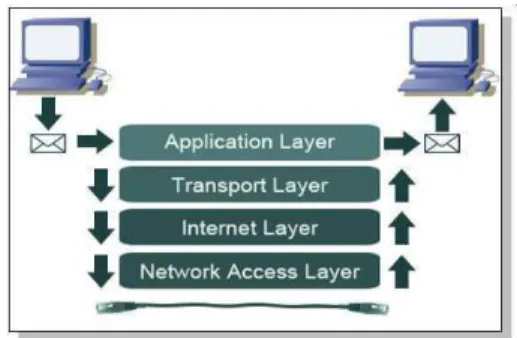
Communication channel between MATLAB (OSIS) and external application Considering the project requirement, the MATLAB program and the external application will be setup in separate computers. Therefore, it is important to implement the data transmission channel for the server/client communication. In this case, using the TCP/IP protocol via a local network to build the
communication channel is an acceptable option. TCP/IP protocol maps two computers under a network and addresses messages so they can be delivered correctly. Nevertheless, transfer speed and network stability should be
considered.
The Polaris ship handler and the OSIS/IHI module are to be installed on two computers separately. In order to connect two computers directly to build the communication channel, the simplest, easiest, and cheapest connection is through a Category 5 ETHERNET crossover cable (Figure 3.1). After connecting them through a crossover cable, users can map two computers via IP
addressing. A communication interface needs to be developed to control the data transaction.
TCP/IP communication based on Java
MATLAB has the capability to execute un-compiled Java code from the
command window. Figure 3.2 shows an example of executing Java codes under MATLAB. To operate the TCP/IP communication, MATLAB needs to import several Java packages. The MATLAB program can utilize the Java Socket and Input/Output Stream classes to control the data transmission via TCP/IP sockets. On the server side, it creates a ServerSocket that provides a Socket around which a DataOutputStream is wrapped and sent to the client once an incoming connection request has been accepted. The client creates a socket to connect to the specified host and port, which provides an input stream that can be wrapped in a DataInputStream from which to read incoming data.
3.2 Design Based on Requirements
According to the requirements specified in the previous section, the
communication channel was built through the local network. In order to examine the feasibilities of the communication protocol, functions based on the Java classes are utilized as the handlers in the communication program. When the connection between OSIS and CMS’s application is implemented,
synchronization is important and it is necessary to employ a “hand-shaking dialogues” to data transmit functions to guarantee transmission reliability, ordering, and data integrity. The basic concept of the design is given in the Figure 3.3.
Figure 3.3: Communication path diagram
As mentioned in the previous section, Java classes can be imported into the MATLAB program and Java functions can be executed under the MATLAB environment. The current demonstration of the communication interface utilizes two Java classes: java.net and java.io. The java.net package provides the
features for the creation and use of Internet Protocol (IP). On IP networks, hosts use the IP address as the basic addressing scheme to target the destinations of messages so that they can be delivered correctly. This scheme is supported directly in the Java’s API (Application Programming Interface). A given host computer on an IP network has a hostname and a numeric address. Either of these, in their fully qualified forms, is a unique identifier for a host on the network.
The communication interface uses the Socket class, which is included in the
java.net package to create TCP connections over an IP network. To create a
Socket, the IP address is used to specify the remote host and a port number to which the host can connect. The remote host is always listening on the given port for incoming connection requests. This process is done in the program using a ServerSocket, which is a built-in function in the Socket class. On the client side, the code simply creates a socket to connect to the remote host on the specified port.
Once a connection between the Client/Server is implemented over the network, Java provides the methods to send and receive data in different formats over the connection through the classes in the java.io package. The communication
interface uses Java classes, InputStream and Outputstream, included in the
java.io package. The InputStream and OutputStream classes can handle data as bytes, with basic methods for reading and writing bytes and byte arrays. Their sub-classes can connect to various sources and destinations, and provide methods for directly sending and receiving data with basic java data types. A Socket, once it is created, can be queried for its input/output streams using
getInputstream and getOutputstream. These methods return instances of
InputStream and OutputStream, respectively.
The communication interface employs two channels, the data channel and the message channel, between the client and the server. They can act as a “ hand-shaking dialogues” handler in the program. The host computer opens two ports for the client to build two TCP channels. Each channel consists of an input
stream and an output stream. For two computers sending data to each other over a TCP socket, they must know the host name and port number of each other’s socket connection. So they will either have preordained ports for each other to create a TCP socket using these ports, or create the socket randomly from a local port and send the port number to each other.
Once the communication between the server and the client is established, two issues must be considered in the scheme of the communication interface: the format of messages and the synchronization. As per requirement, the ship motions and the ice forces are major information needed by both server and client computation. Hence, most of the data are arrays with double precision numbers of many decimal digits. In order to transmit this data efficiently and accurately, they are converted to ASCII strings before transfer. The java.io
package provides the function to write the entire string to an OutputStream; however, when the server/client receives the incoming data, it can only read the data byte by byte. Furthermore, the receiver needs to convert the received data from the ASCII string to double precision or the type they used to be. Every piece of data has a unique ID. When the data is sent from the server to the client
through the data channel, its ID is sent concurrent to the client through the message channel as a notification. The server will wait for a response message from the client before sending the next stream of data. With the notification and response, the data transaction between the server and client is synchronized.
4 THE DEMONSTRATION OF THE MATLAB COMMUNICATION 4.1 The MATLAB Communication Facility
This version of MATLAB communication interface was developed for
demonstration purposes and its main structure is based on OSIS-IHI. The IHI module was extracted from the OSIS-IHI software to form a stand-alone application. This module was installed on the client computer, and the data transfer functions, based on Java classes, were developed for client operations. For demonstration purposes, the IHI module, that is to be integrated into the Polaris software, is activated on computer #2 and it simply passes the computed ice force to OSIS that is activated on computer #1 to mimic the Polaris
applications by providing the GUI and the motion solver. The OSIS is hotwired to by-pass IHI computation; instead, it communicates with the client for ice force computation. The module to handle server operations has been integrated with the OSIS and it is invoked when the user starts OSIS.
So far the demonstration of the communication interface is an un-compiled version and it has to be running under the MATLAB environment. A compiled version of this demonstration will be available on a later date. It will allow the users to run this communication interface as a stand-alone application without MATLAB. A step-by-step direction for MATLAB compiler is documented in the Appendix C.
4.2 File List for The Communication Interface
The following lists the files used in the demonstration of the communication interface. These files can be modified according to the design requirement. Also, the input and output variables of the current communication interface are listed in the Appendix A1. A programmer manual of the communication interface including codes and comments is listed in the Appendix B.
The SERVER
The server part of the demonstration includes the main structure of OSIS that bypasses the IHI module. Several files for the communication operations are listed below:
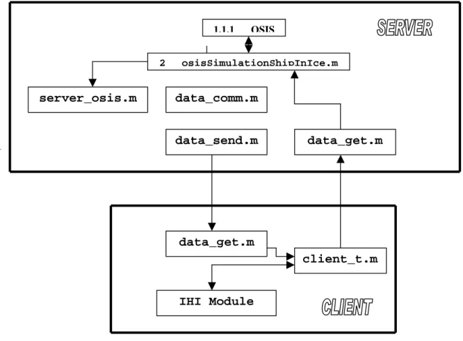
server_osis.m – It opens two ports on the server and generates the output and
feedback stream on each port. This function is called at the beginning of osisSimulationShipInIce.m, which handles the main operation for simulation of the Ship-in-Ice Model. The Ship-in-Ice Model is set as the default simulation task in the demonstration.
data_comm.m – This function is also called in osisSimulationShipInIce.m. It collects input variables for IHI on the server side. For each variable, the function data_send.m is called to send the variable from the server to the client.
data_send.m – This function is called in data_comm.m. It sends the input
variables from the server to the client.
data_get.m – This function is called in osisSimulationShipInIce.m. It receives the
calculation results from the client.
The CLIENT
The IHI module receives motion data from the server and sends the computed ice forces back to the server. The following lists the functions operating the data input/output:
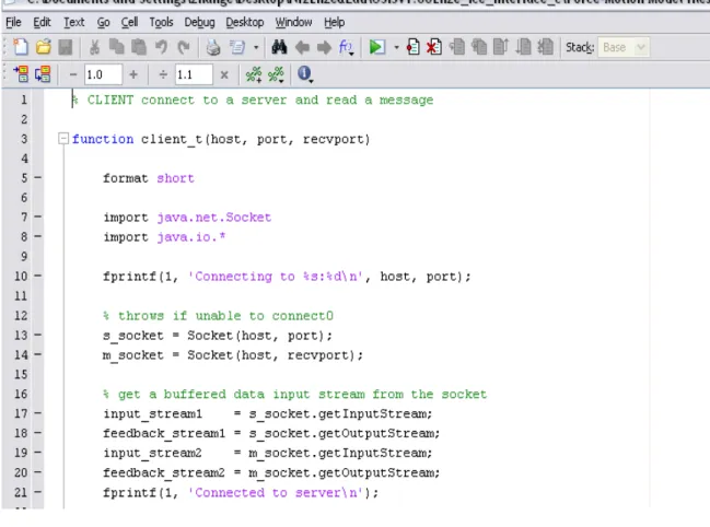
client_t.m – This is the main function of the client part of the communication
interface. After starting OSIS on the server side, this function is called on the client side to establish the connection with the server. This function will keep running until the end of the simulation. In the first time step, this function receives the initial variables from the server to initialize the IHI module. Then it collects the incoming data from the server, calls the IHI module to calculate the ice forces, and sends the computational results back to the server for each time step.
data_get.m – This function is called in client_t.m. It receives the incoming data
from the server.
Figure 4.1 is the flow chart showing the operating process of the communication interface.
4.3 Validation
In this demonstration of the communication interface, the input data file and the configuration are same as an OSIS simulation task, Healy1shipInIce (The input data file is given in the Appendix A2). The computation accuracy of the
demonstration is verified by comparing its calculation result with the OSIS simulation result of Healy1shipInIce. As was expected, the results from the demonstration and the OSIS simulation are the same. That approves the validation of the IHI module’s computation in the current demonstration. The following lists the graphic result of OSIS simulation and the current
demonstration, which includes the water line, track of ship in ice motion, Z-axis moment, and the X-Y velocity. These results are simulated within 256 time steps. The ship motion in the simulation has already entered the steady state, and the
Figure 4.1: Flow chart of the communication interface
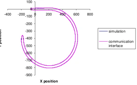
Figures 4.2 and 4.3 present a comparison of the ship’s waterline and ship’s track between the interface version and the stand-alone version of the OSIS-IHI, which shown a good agreement between these two versions.
1.1.1 OSIS 2 osisSimulationShipInIce.m server_osis.m data_comm.m data_send.m data_get.m client_t.m data_get.m IHI Module
Figure 4.2: Comparison of ship’s waterline
Figure 4.3: Comparison of ship’s track
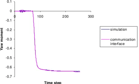
Figures 4.4, 4.5 and 4.6 further compare the surge velocity (Vx), sway velocity (Vy)
and yaw moment (Mz) simulated by the interface version to those by the
stand-alone versions, respectively. These results show large errors occurring during the transient state of the ship motion (i.e., the beginning of the simulation) especially with the sway velocity (Figure 4.5) and the yaw moment (Figure 4.6). However, the errors are reduced significantly in the steady state as shown in Figure 4.7 that gives the percentage error versus time step for the yaw moment simulated during steady state.
-900 -800 -700 -600 -500 -400 -300 -200 -100 0 100 -400 -200 0 200 400 600 800 X position Y p o s it io n simulation communication interface -100 0 100 200 300 400 500 600 700 800 900 -400 -200 0 200 400 600 800 X position Y p o s it io n simulation communication interface
Figure 4.4: Comparison of surge (X) velocity
Figure 4.5: Comparison of sway (Y) velocity
-2 -1 0 1 2 3 4 5 0 50 100 1 50 20 0 250 3 00 Time st ep V e lo c it
y X v eloc ity (Com m unic atio n
inter fa ce )
X v eloc ity (Sim u la tion r es ult)
-5 -4 -3 -2 -1 0 1 0 50 10 0 150 2 00 25 0 300 Time st ep Y v e lo c it
y Y v eloc ity ( Com m unic atio n
in te rfac e)
Figure 4.6: Comparison of yaw moment (Mz)
Figure 4.7: Percentage error versus time step for the yaw moment (steady state portion) -0.7 -0.6 -0.5 -0.4 -0.3 -0.2 -0.1 0 0.1 0 100 200 300 Time step Y a w m o m e n t simulation communication interface -1 -0.8 -0.6 -0.4 -0.2 0 0.2 0.4 0.6 0.8 1 116 166 216 266 Time step P e rc e n ta g e e rr o r (% )
Figure 4.8: Percentage error for X & Y-velocity comparison
Figure 4.7 presents the percentage errors for Yaw moment from time step 116 to 256, in which the ship motion is in the steady state. The percentage error in this time interval is within the range of 0 to –0.8%. Figure 4.8 presents the
percentage errors for X & Y-velocity from time step 90 to 256. It can be seen that the percentage error remains in a very low level (under 1%). Only two time steps in the X-velocity give significant errors. These errors occur due to the mismatch during the data transaction, but this type of error rarely happen in the simulation and would not affect the final simulation result. Since the purpose of the
simulation is focused on the steady state, as long as the results of steady state retain its accuracy, the errors occur during the transient state will not be
considered as an issue in the development.
Comparison between the results of the demonstration and the OSIS simulation can only constitute an indirect verification. In order to verify the accuracy and reliability of the data transaction, each data pack needs to be checked to determine if it is delivered successfully from one end to the other.
-50 -40 -30 -20 -10 0 10 20 30 40 50 90 140 190 240 Time step P e rc e n ta g e e rr o r (% ) Percentage error of X velocity Percentage error of Y velocity
Figure 4.9: Data transaction difference (ice force)
Figure 4.9 shows the percentage difference of data in two ends of transaction. The graph is generated based on the total ice force, which is transmitted from the client to the server from time step 1 to 347. The curve indicates that most of the data packages show no difference before and after the transaction. Differences only occur twice out of 347 time steps and the largest difference is less than 3.5%. These errors were caused by missing bytes during the transaction; however, considering their minimal impact on the final simulation result, they should not be an issue for the communication interface.
Therefore, based on the above assessment, the current demonstration can guarantee the accuracy of the data transaction. During the demonstration, every data package is displayed in the command window on both server and client computers, and the users can easily verify that data is sent and received
correctly. It needs to be pointed out that the transaction accuracy is highly related to the size of each data package in the current demonstration. Because there will be more discussions on the design requirements with CMS, it is anticipated that the data transaction scheme will be modified. Therefore, it is necessary to keep updating the validation of the data transaction.
-0. 005 0 0. 005 0.01 0. 015 0.02 0. 025 0.03 0. 035 0.04 10 60 110 160 210 260 310 Time step E rr o r p e r c e n ta g e
4.4 Estimation of an Alternative Communication Scheme
Figure 4.10 is the timing diagram of the simulation process in the current demonstration. The process line bases on a single thread operating in a sequential manner. After completing its own task, it has to pause for the other party to complete its task before proceeding to next time step.
Time step 0 1 2 3 OSIS M0 F0 ->M1 F1->M2 F2->M3 Data transmit M0 F0 M1 F1 M2 F2 IHI M0->F0 M1->F1 M2->F2
Figure 4.10: Time diagram of communication process
In order to increase the process speed of the communication interface, a new communication scheme has been developed. Figure 4.11 show a schematic of the communication new scheme.
Time step 0 1 2 3 4 3 OSIS M0 F0 ->M1 F1=F0 ->M2 F2->M3 F3->M4 F4->M5 Data transmit M0 F0,F1 M1 F2 M2 F3 M3 F4 M4 IHI M0-> F0=F1 M1-> F1=F2 M2-> F2=F3 M3-> F3=F4 M4-> F4=F5
Figure 4.11: Timing diagram of the alternative communication scheme
In the simulation of ship motion, especially the straight forward and turning circle motions, it is possible to assume that the current ice force is very close to, or equal to the ice force in the previous time step. Based on the assumption of current ice force Ft = Ft-1, the OSIS can use the previous ice force to compute the ship motion when it is waiting for the calculation result from IHI module. It sends the computational result of ship motion immediately and fetches the ice force from IHI module in the meantime. In this case, the delay time for the server’s computation is removed from the processing stream. Therefore, the simulation speed of the integration facility can be increased. However, the assumption of Ft = Ft-1 introduces errors. If motion change is small between
consecutive time step, errors may also be small. If the errors can be controlled in a reasonable range, this communication scheme is acceptable. Nevertheless, more verification is needed to assess the reliability of the new scheme.
4.5 Result of Preliminary Assessment
Based on the preliminary assessment of the communication interface, the communication between OSIS and other external applications, such as Polaris, should be feasible via network connections and MATLAB’s communication protocols. In the demonstration, the input data are split into 30 data packages during the first time step of the simulation and sent to the IHI module one by one to initialize the ice force calculations. After the initialization, only four data
packages will be sent to the client in each step of the simulation: index, step, motion, and time control. All these data are reconstructed to different types of variables by the client and the calculation result, i.e., ice force, is sent back to the server to continue the simulation. In the demonstration, the ice force includes two components, the global ice force on the whole ship and the local ice force on each hull point profiling the ship’s waterline geometry. On the server side, OSIS only needs the global ice force to continue the simulation; however, the ice force on each hull point will be employed when the Polaris ship handler replaces the OSIS as the server. Depending on the hull definition, the hull can be defined by many hull points. If the Polaris ship handler employs the entire data set of the ice force on each hull point, it will take a greater length of time to process during the simulation due to the large size of the data package. New routines will need to be developed to handle this issue.
In order to ensure the synchronization of the client/server operation, there is a short delay time applied in each simulation time step. This delay time is related to the network speed and the CPU speed. The delay time guarantee that two ends of the communication can finish the data transaction during the simulation and no data is missed. However, it leads to a speed issue. The simulation will be slowed down due to the delay time imposed at each time step. In addition, both server and client need time to finish their calculation. Thus, they need a handler to operate the data transaction so that the server and the client can be
synchronized. In the current demonstration, instead of giving a fixed delay time, a routine is built-in on both the server and client sides of the communication
interface. This routine can check if there are data package available in the communication channel. It then holds the server/client until there is a complete data package delivered to them.
The speed issue is present in the demonstration testing. Not only the delay time in the data transaction, but also the time required for calculation will increase as
all, the speed issue is not difficult to improve, whereas, the synchronization is more critical for the integration facility.
5 RECOMMENDATION FOR FURTHER INTEGRATION EFFORT
A demonstration of MATLAB’s communication interface was developed using OSIS and IHI as independent modules or applications. It presents some basic features that can handle the external data transfer between MATLAB and other applications. It is anticipated that the java classes utilized in this demonstration would be helpful in the further development of the actual interface between the IHI module and the Polaris application. This investigation assesses the possibility of potential solutions for this IHI-Polaris interface with the pertinent issues and challenges identified for further effort.
In this demonstration, the input and output data are arranged based on the assumption that the Polaris application passes motion information to the IHI module and gets ice force prediction back from it. In MATLAB, these data can be wrapped as data packages of doubles and transmitted via java functions byte by byte. The current investigation has demonstrated the data transfer between the IHI and an external application is satisfactory within the MATLAB environment; however, it is not sufficient to verify that this scheme fully satisfies CMS’s requirements. CMS needs to supply specific information, including input/output data name, type, size, and the external communication protocol used by the Polaris application, before a more in depth assessment is possible.
It is possible to consider a more efficient communication scheme, especially in situations when several different types of data are to be transferred between the client and the server. As mentioned in the previous section, each set of input data is packed into one data package and sent one by one in the communication process. This may lead to speed issues during simulation. If all input data can be wrapped into one data package, it can significantly improve the simulation speed. In MATLAB, different types of variables can be transferred to ASCII numbers and saved to a package in a certain format. The package can be transmitted to the client and then decoded based on that format. Several items, such as the order and size of data, remain unchanged in every simulation time step. Hence, it is possible to use this information to decode the transferred data
The integration between OSIS-IHI and Polaris is a co-operative effort between IOT and CMS who need to compile their respective resource and design specification to specify more design details. In order to accelerate the interface development, the following lists three key points that require agreements between IOT and CMS:
Overall integration scheme
Refer to Section 2, there are three integration options between OSIS-IHI and the Polaris ship handler. Option One was selected and demonstrated as the most
IOT need to reach the agreement on one of the integration scheme before looking into more details.
The communication protocol
IOT needs to have the discussion with CMS on the implementation of the communication via TCP/IP protocol. Alternatively there may be other solutions that better match the design requirement. In addition, CMS should provide more information on Polaris’ I/O capabilities.
The input/output data
So far the data set selected for transfer are for demonstration purposes. IOT and CMS need to agree on a complete set of data (ship particulars, ice conditions, ship motion and ice force) that need to be transferred in the various integration schemes (i.e., IHI – Polaris, OSIS-IHI – Polaris, and OSIS-IHI – Kongsberg). This is the critical issue because the design of the communication scheme is
6 REFERENCES
Lau, M and Ni, S.Y., 2009. “Ship Manoeuvring in Ice Simulation Software OSIS-IHI”, IOT Report LM-2009-02, Institute for Ocean Technology, National Research Council of Canada, St. John’s, Newfoundland.
Lau. M., 2009, Suggested Options for OSIS-IHI/Kongsberg Interface, a communication to CMS, St. John’s Newfoundland.
Farley, J., 1998. JAVA Distributed Computing. 1st Edition, Edited by Mike Loukides, O'Reilly & Associates, Inc. Sebastopol, CA, USA
Appendix A
A.1 Data communication between OSIS (server side) and IHI (client side)
Server to client:
The following variables is sent from the server to client in every time step:
is_openwater boolean value
step integer index integer
Motion double, 1x6 matrix
Time_contr double, 1x3 matrix
The following are three MATLAB structures, Simpl_model, Prope_ice, and
Prope_ship. They are only sent to client to initialize the IHI module in the first time step.
Example: Simpl_model =
Geo: [1 7 9 11 14 17 21] Prope: [1x1 struct]
Simpl_model.Geo integer, 1x7 matrix
Simpl_model.Prope.Bow double, 1x10 matrix
Simpl_model.Prope.Mid_body double, 1x9 matrix
Simpl_model.Prope.Stern double, 1x7 matrix
Example: Prope_ice = Stren: [1.0058e+009 519000 1557000 1038000 0.3300] Const: [1.9272 0.7490 1002 870 9.8070 1] Veloc: [0.7500 0.3000] Frict: [0.0340 0.0340] Model: 1
Prope_ice.Stern double, 1x5 matrix
Prope_ice.Const double, 1x6 matrix
Prope_ice.Veloc double, 1x2 matrix
Prope_ice.Frict double, 1x2 matrix
Prope_ice.Model integer
Example:
Prope_ship =
Geo: [1x1 struct]
Mass: [1.5049e+007 58.7300 0 -1.2818 9.3681e+008 1.3780e+010 1.3780e+010]
Dimen: [120.8500 24.9900 8.5300 8.5300 24 32 60] Model: 1
Prope_ship.Motio double, 1x8 matrix
Prope_ship.Mass double, 1x7 matrix
Prope_ship.Dimen double, 1x7 matrix
Prope_ship.Model integer
Prope_ship.Geo.Water_line double, 55x5 matrix
Prope_ship.Geo.is3d boolean value
Prope_ship.Geo.bow_type integer
Prope_ship.Geo.bow_wl double, 55x3 matrix
Prope_ship.Geo.start integer Prope_ship.Geo.end integer Prope_ship.Geo.imid1 integer Prope_ship.Geo.imid2 integer Prope_ship.Geo.imin integer Prope_ship.Geo.dmin integer Prope_ship.Geo.dcent integer Prope_ship.Geo.imin2 integer Client to server:
Hull_ice_force double, 1x6 matrix
Ice_total_froce_each_point double, 55x6 matrix (converted to 1 row array during transaction)
A.2 Initial input data for OSIS
Ship in Ice settings configuration file Created on Mar 10, 2008
Explainations for the input data:
1)Afterbody Form: Cstern: 0 Normal section shape, 10 U-shaped sections with Hogner stern
-10 V-shaped sections, -25 Pram with gondola
2)Ship Gyradius Radius (m): sqrt(Ship Gyradius Ixx, Iyy, Izz/Ship Mass) 3)Surface Normal to Vertical Direction Angle (deg): not on station section 4)C1 Velocity:0.75 C2 velocity:0.3 for
5)Appendages: form factor 1+k2
Rudder behind skeg 1.5 - 2.0 Rudder behind stern 1.3 - 1.5 Twin-screw balance rudders 2.8
Hull bossings 2.0 Shafts 2.0 - 4.0 Stabilize fins 2.8 Dome 2.7 Bilge keels 1.4
6)Ship Wetted Surface could be set -1 when unkown
7)Outputfilename.ood is a binary file to save results for GUI ---
Output filename = OSIS Outputs\HealyInIce.ood Simulation length (s) = 1500 Time Increment (s) = 00001 Ship Length (m) = 120.85 Ship Width (m) = 24.99 Ship Draught (m) = 8.53 Scale (ship/model) = 1.0 Block Coefficient Cd = 0.583 Prismatic Coefficient Cp = 0.649 Midship Section Coefficient Cm = 0.898 Waterline Area Coefficient Cwp = 0.818
Longitudinal Center of Buoyance (%L forward of AP) = 48.794 Transverse Transom Area (m^2) = 0.0
Transverse Bulb Area (m^2) = 0.0 Bulb Center above Keel Line (m) = 0.0
Ship Gravity Centre (forward of AP)(m) = 57.2193 00000 -1.2818 Ship Gyration Radius (m) = 7.89 45.26 45.26 Ship Wetted Surface (m^2) = 3677.59
Waterline Entrance Angle (deg) = 44.17 Stem Angle (deg) = 21.9 Surface Normal to Vertical Direction Angle (deg) = 00060 Afterbody Form Type = 0
Water Density (kg/m^3) = 01002 Ice Density (kg/m^3) = 00866 Ice Thickness (m) = 0.749 Ice Flexural Strength (Pa) = 519000 Ice Compressive Strength (Pa) = 1557000 Ice Shear Strength (Pa) = 1038000 Poisson's Ratio = 3.30000e-001 Young's Modulus (Pa) = 1038000000 Velocity Effect to Ice Piece Size C1 = 0.75
Velocity Effect to Ice Piece Size C2 = 0.3 Dynamic Friction of Hull-Ice = 0.05 Static Friction of Hull-Ice = 0.05
Rudder Height (m) = 5.4663 Rudder Length (m) = 3.354
Rudder Number = 2 Rudder Centre (forward of AP)(m) = 4.6615 Propeller Diameter (m) = 4.708 Propeller Pitch Ratio = 0.775 Propeller Blade Number = 4 Propeller Number = 2 J-Kt, 10Kq, eta0 (Propeller 66) Number of J = 43 J1 = 0 0.349 0.403 0 J2 = 0.02 0.343 0.398 0.027432234 J3 = 0.04 0.338 0.393 0.05475254 J4 = 0.06 0.332 0.387 0.081921614 J5 = 0.08 0.325 0.382 0.108325354 J6 = 0.1 0.319 0.376 0.135027731 J7 = 0.12 0.312 0.37 0.161047596 J8 = 0.14 0.305 0.364 0.186700991 J9 = 0.16 0.298 0.358 0.211969488 J10 = 0.18 0.291 0.342 0.24375836 J11 = 0.2 0.283 0.346 0.260351728 J12 = 0.22 0.276 0.339 0.285070447 J13 = 0.24 0.268 0.333 0.307412791 J14 = 0.26 0.26 0.326 0.330026815 J15 = 0.28 0.253 0.32 0.352329255 J16 = 0.3 0.244 0.314 0.371023625 J17 = 0.32 0.236 0.307 0.391510792 J18 = 0.34 0.229 0.299 0.414441601 J19 = 0.36 0.221 0.292 0.433642715 J20 = 0.38 0.213 0.285 0.452000038 J21 = 0.4 0.205 0.278 0.469449832 J22 = 0.42 0.197 0.271 0.485921771 J23 = 0.44 0.189 0.264 0.501338071 J24 = 0.46 0.181 0.256 0.517626584 J25 = 0.48 0.173 0.249 0.530772148 J26 = 0.5 0.165 0.242 0.54257367 J27 = 0.52 0.157 0.234 0.555273913 J28 = 0.54 0.149 0.226 0.566619766 J29 = 0.56 0.141 0.219 0.573829877 J30 = 0.58 0.133 0.211 0.581858403 J31 = 0.6 0.125 0.203 0.588010873 J32 = 0.62 0.117 0.194 0.595108225 J33 = 0.64 0.108 0.186 0.591440305 J34 = 0.66 0.1 0.177 0.59345911
J38 = 0.74 0.064 0.14 0.538398436 J39 = 0.76 0.055 0.13 0.511744355 J40 = 0.78 0.045 0.12 0.465528209 J41 = 0.8 0.035 0.109 0.408838386 J42 = 0.82 0.025 0.098 0.332926156 J43 = 0.84 0.014 0.087 0.215133578
Appentage wetted surface, 1+k2 Number of appendage = 1 app1 = 140.0 3.0
Hull Dimension = 2d Number of Hull points = 55
1 =1.5107 -4.4888 0 40.52250726 1.564887365 2 =3.02133 -5.64984375 0 47.93941972 5.827901616 3 =6.04266 -7.3726875 0 49.17602192 5.26754282 4 =9.06399 -8.63971875 0 51.96792565 4.815050379 5 =12.08532 -9.50034375 0 56.09408584 4.477544875 6 =15.10665 -10.11553125 0 61.77560485 4.158927938 7 =18.12798 -10.6111875 0 67.32282634 15.77766456 8 =24.17064 -11.34271875 0 72.51097486 36.37103427 9 =30.2133 -11.81765625 0 77.064605 47.11297806 10 =36.25596 -12.07425 0 79.60770971 45.13127855 11 =42.29862 -12.157125 0 80.10322788 45.07135043 12 =48.34128 -12.16828125 0 79.99416577 45.06270111 13 =54.38394 -12.16828125 0 80.03032805 45.06270111 14 =60.4266 -12.16828125 0 79.93997783 45.10328925 15 =66.46926 -12.157125 0 79.50755248 45.51874362 16 =72.51192 -12.11409375 0 78.57485054 47.16587864 17 =78.55458 -12.0615 0 76.78930573 51.01471818 18 =84.59724 -11.97065625 0 73.04520144 57.33865484 19 =90.6399 -11.7140625 0 66.66635446 65.50508347 20 =96.68256 -10.98571875 0 59.80389411 35.83077602 21 =99.70389 -10.3561875 0 54.54831947 36.73207606 22 =102.72522 -9.5656875 0 50.08535364 18.2204706 23 =105.74655 -8.5201875 0 46.0016416 20.03024012 24 =108.76788 -7.22765625 0 42.4871178 13.80374177 25 =111.78921 -5.7151875 0 39.15312642 7.104946063 26 =114.81054 -4.0449375 0 35.95296515 5.81056795 27 =117.83187 -2.16590625 0 33.68924791 2.067059338 28 =120.8532 0 0 20.23230631 2.067059338 29 =117.83187 2.16590625 0 33.68924791 5.81056795 30 =114.81054 4.0449375 0 35.95296515 7.104946063 31 =111.78921 5.7151875 0 39.15312642 13.80374177 32 =108.76788 7.22765625 0 42.4871178 20.03024012 33 =105.74655 8.5201875 0 46.0016416 18.2204706
34 =102.72522 9.5656875 0 50.08535364 36.73207606 35 =99.70389 10.3561875 0 54.54831947 35.83077602 36 =96.68256 10.98571875 0 59.80389411 65.50508347 37 =90.6399 11.7140625 0 66.66635446 57.33865484 38 =84.59724 11.97065625 0 73.04520144 51.01471818 39 =78.55458 12.0615 0 76.78930573 47.16587864 40 =72.51192 12.11409375 0 78.57485054 45.51874362 41 =66.46926 12.157125 0 79.50755248 45.10328925 42 =60.4266 12.16828125 0 79.93997783 45.06270111 43 =54.38394 12.16828125 0 80.03032805 45.06270111 44 =48.34128 12.16828125 0 79.99416577 45.07135043 45 =42.29862 12.157125 0 80.10322788 45.13127855 46 =36.25596 12.07425 0 79.60770971 47.11297806 47 =30.2133 11.81765625 0 77.064605 36.37103427 48 =24.17064 11.34271875 0 72.51097486 15.77766456 49 =18.12798 10.6111875 0 67.32282634 4.158927938 50 =15.10665 10.11553125 0 61.77560485 4.477544875 51 =12.08532 9.50034375 0 56.09408584 4.815050379 52 =9.06399 8.63971875 0 51.96792565 5.26754282 53 =6.04266 7.3726875 0 49.17602192 5.827901616 54 =3.02133 5.64984375 0 47.93941972 1.564887365 55 =1.5107 4.4888 0 40.52250726 17.02568966
APPENDIX B
THE PROGRAMMER MANUAL
In this programmer manual, it lists m-files of the current demo.
Server (OSIS) data_comm.m :
function data_comm(output_stream1, output_stream2,feedback_stream, is_openwater,motion, index, step, Prope_ship,Prope_ice,Simpl_model,Time_contr)
%---
% This function is currently embedded with osisSimulationShipInIce.m. This % is the main function to handle the operations of sending data packages % from server to client. Eventually, this function or a function wih a % similar structure will be implemented with the CMS server application, % Polaris ship handler.
%
% This function needs the following inputs: % output_stream1 - implement the data channel % output_stream2 - implement the msg channel
% others - the rest of input parameters are required by IHI model to % initialize its simulation.
% Note: index, step, motion, Time_contr will be send to IHI module in % every time step. Others will only be sent in the first time step. %
% Function data_send.m is called to send the datapackages to the client. %---
disp('======= Start data communication test ========');
%The following three parameters - index, motion, Time_contr, are sent %from server to the client in every time step
index = uint32(index);
s_index = num2str(index); %convert number to string %send data
data_send(output_stream1, output_stream2,feedback_stream,s_index, '03'); s_motion = num2str(motion); %convert number to string
%send data
data_send(output_stream1,output_stream2, feedback_stream,s_motion,'04'); s_time = num2str(Time_contr); %convert number to string
%sent data
data_send(output_stream1, output_stream2,feedback_stream,s_time, '05'); if index == 1,
% The following parameters will only be sent in the first time step (index=1) % to initialize the IHI module
%convert the boolean value to integer if is_openwater == true,
op_water = uint8(1); else
op_water = uint8(0); end
%send data
data_send(output_stream1,output_stream2, feedback_stream,op_water,'01');
step = uint8(step);
s_step = num2str(step); %convert number to string %send data
data_send(output_stream1,output_stream2, feedback_stream,s_step, '02');
%---
% The following are three MATLAB structures, Simple_model, % Prope_ice, Prope_ship.
% In order to send a MATLAB structure, we break variables in each % structure to single parameters and send them in order. They will % be re-constructed when the client receives them.
%---
%Simpl_model
s_geo = num2str(Simpl_model.Geo); %convert number to string % disp(s_geo);
%send data
data_send(output_stream1, output_stream2,feedback_stream,s_geo, '06'); s_bow = num2str(Simpl_model.Prope.Bow); %convert number to string % disp(s_bow);
%send data
data_send(output_stream1,output_stream2, feedback_stream,s_bow, '07');
s_mid_body = num2str(Simpl_model.Prope.Mid_body); %convert number to string % disp(s_mid_body);
%send data
data_send(output_stream1, output_stream2,feedback_stream,s_mid_body, '08'); s_Stern = num2str(Simpl_model.Prope.Stern); %convert number to string % disp(s_Stern);
%send data
data_send(output_stream1,output_stream2, feedback_stream,s_Stern, '09'); %Prope_ice
s_ice_stern = num2str(Prope_ice.Stren); %convert number to string % disp(s_ice_stern); %send data data_send(output_stream1,output_stream2, feedback_stream,s_ice_stern, '10'); s_ice_Const = num2str(Prope_ice.Const); % disp(s_ice_Const); data_send(output_stream1,output_stream2, feedback_stream,s_ice_Const, '11');
s_ice_Veloc = num2str(Prope_ice.Veloc); %convert number to string % disp(s_ice_Veloc);
%send data
data_send(output_stream1, output_stream2,feedback_stream,s_ice_Veloc, '12'); s_ice_Frict = num2str(Prope_ice.Frict); %convert number to string
% disp(s_ice_Frict); %send data
data_send(output_stream1, output_stream2,feedback_stream,s_ice_Frict, '13');
%Prope_ship
s_motio = num2str(Prope_ship.Motio); %convert number to string % disp(s_motio);
%send data
data_send(output_stream1,output_stream2, feedback_stream,s_motio, '15'); s_mass = num2str(Prope_ship.Mass); %convert number to string
% disp(s_mass); %send data
data_send(output_stream1,output_stream2, feedback_stream,s_mass, '16'); s_dimen = num2str(Prope_ship.Dimen); %convert number to string % disp(s_dimen);
%send data
data_send(output_stream1,output_stream2, feedback_stream,s_dimen, '17'); s_ship_model = uint8(Prope_ship.Model);
s_ship_model = num2str(s_ship_model); %convert number to string % disp(s_ship_model);
%send data
data_send(output_stream1,output_stream2, feedback_stream,s_ship_model, '18');
% disp(Prope_ship.Geo.Water_line);
% Note: ship water_line is a 55x5 array. The "write" function % requires a single row array. Therefore, we need to convert it to % a 1x275 array l_w = size(Prope_ship.Geo.Water_line); len_w = length(Prope_ship.Geo.Water_line); h_w = zeros(1, len_w); k = 1; for i = 1:l_w(2) for j = 1:l_w(1) h_w(k) = Prope_ship.Geo.Water_line(j,i); k = k+1; end end
s_h_w = num2str(h_w); %convert number to string %send data
data_send(output_stream1,output_stream2, feedback_stream,s_h_w, '19');
%convert boolean value to number if Prope_ship.Geo.is3d == true, is3d = uint8(1);
else
is3d = uint8(0); end
is3d = num2str(is3d); %convert number to string %send data
data_send(output_stream1, output_stream2,feedback_stream,is3d, '20'); s_bow_t = uint8(Prope_ship.Geo.bow_type);
s_bow_t = num2str(s_bow_t);
data_send(output_stream1, output_stream2,feedback_stream,s_bow_t, '21'); %Note: Same as ship water_line, this is a 55x3 array, it needs to
%be convert to a single row array size_wl = size(Prope_ship.Geo.bow_wl); len_wl = length(Prope_ship.Geo.bow_wl); h_wl = zeros(1, len_wl);
q = 1;
for g = 1:size_wl(1)
h_wl(q) = Prope_ship.Geo.bow_wl(g, f); q = q + 1;
end end
s_h_wl = num2str(h_wl); % convert number to string %send data
data_send(output_stream1, output_stream2,feedback_stream,s_h_wl, '22'); s_start = uint8(Prope_ship.Geo.start);
s_start = num2str(s_start); %convert number to string %send data
data_send(output_stream1,output_stream2,feedback_stream, s_start, '23'); s_end = uint8(Prope_ship.Geo.end);
s_end = num2str(s_end); %convert number to string %send data
data_send(output_stream1, output_stream2,feedback_stream,s_end, '24'); s_imid1 = uint8(Prope_ship.Geo.imid1);
s_imid1 = num2str(s_imid1); %convert number to string %send data
data_send(output_stream1, output_stream2,feedback_stream,s_imid1, '25'); s_imid2 = uint8(Prope_ship.Geo.imid2);
s_imid2 = num2str(s_imid2); %convert number to string %send data
data_send(output_stream1, output_stream2,feedback_stream,s_imid2, '26'); s_imin = uint8(Prope_ship.Geo.imin);
s_imin = num2str(s_imin); %convert number to string %send data
data_send(output_stream1,output_stream2, feedback_stream,s_imin, '27'); s_dmin = uint8(Prope_ship.Geo.dmin);
s_dmin = num2str(s_dmin); %convert number to string %send data
data_send(output_stream1,output_stream2, feedback_stream,s_dmin, '28'); s_dcent = uint8(Prope_ship.Geo.dcent);
s_dcent = num2str(s_dcent); %convert number to string %send data
data_send(output_stream1, output_stream2,feedback_stream,s_dcent,'29'); s_imin2 = uint8(Prope_ship.Geo.imin2);
s_imin2 = num2str(s_imin2); %convert number to string %send data
data_send(output_stream1,output_stream2, feedback_stream,s_imin2, '30');
end
% give a short delay time here to finish the data transaction
% Note: this delay time can be adjust shorter or even removed, as long % as the data transaction can work without any problems.
pause(0.05); end
% This function imports several java functions to fetch data from the input % stream. It is called in osisSimulationShipInIce.m to get the ice force % calculation result from the client.
%
% Inputs: input_stream, index
%--- % import java classes
import java.net.Socket import java.io.*
import java.io.InputStream % active the input stream
d_input_stream = DataInputStream(input_stream);
% read data from the socket - must get the entire data package! while true
%check how many bytes of data currently available in the input stream bytes_available = input_stream.available;
% ---
% then the following if-elseif statement is used to ensure the % function can read the entire data package. In the current demo, % the size of ice force is changing during the simulation. Here the % simulation time steps is separated to 3 stages, 0->14, 14->75, % after 75. In each stage, the ice force has a minimum size. % The function keep checking the available data size until % it is large than the minimum size.
%
% NOTE: it is working with the current demo, when you modify the % ice force, this function MUST be modified based on the size of % the ice force.
%
% TO DO: it should have a better way to check the received data % package.
%--- if index < 14 && bytes_available < 32
pause(0.015); continue;
elseif index >=14 && bytes_available < 430 pause(0.015);
continue;
elseif index >=75 && bytes_available < 450 pause(0.015);
continue; else
fprintf(1, 'Reading %d bytes\n', bytes_available); data_rec = [];
%ready data byte by byte for i = 1:(bytes_available/2);
data_rec(i) = d_input_stream.readChar(); end
result = char(data_rec); %convert the result from ASCII to char data_rec = str2num(result); %convert result from string to number
break; end end
end
data_send.m :
function [data_rec] = data_get(input_stream,index) %---
% This function imports several java functions to fetch data from the input % stream. It is called in osisSimulationShipInIce.m to get the ice force % calculation result from the client.
%
% Inputs: input_stream, index
%--- % import java classes
import java.net.Socket import java.io.*
import java.io.InputStream % active the input stream
d_input_stream = DataInputStream(input_stream);
% read data from the socket - must get the entire data package! while true
%check how many bytes of data currently available in the input stream bytes_available = input_stream.available;
% ---
% then the following if-elseif statement is used to ensure the % function can read the entire data package. In the current demo, % the size of ice force is changing during the simulation. Here the % simulation time steps is separated to 3 stages, 0->14, 14->75, % after 75. In each stage, the ice force has a minimum size. % The function keep checking the available data size until % it is large than the minimum size.
%
% NOTE: it is working with the current demo, when you modify the % ice force, this function MUST be modified based on the size of % the ice force.
%
% TO DO: it should have a better way to check the received data % package.
%--- if index < 14 && bytes_available < 32
pause(0.015); continue;
elseif index >=14 && bytes_available < 430 pause(0.015);
continue;
elseif index >=75 && bytes_available < 450 pause(0.015);
continue; else
fprintf(1, 'Reading %d bytes\n', bytes_available); data_rec = [];
data_rec = str2num(result); %convert result from string to number break; end end end server_osis.m :
function [output_stream1, feedback_stream1, output_stream2, feedback_stream2] = server_osis(output_port1,output_port2)
%--- % This function is called at the beginning of the
% osisSimulationShipInIce.m. Eventually this function or a modified % version will be embedded with the server application, Polaris ship % handler.
%
% This function opens two ports for two pairs of input/output streams %---
%import java functions import java.net.ServerSocket import java.io.*
fprintf(1, ['Waiting for client to connect to this ' ...
'host on ports : %d, %d\n'], output_port1, output_port2);
%Create a socket on output_port1, listening connection from the client server_socket = [];
try
server_socket = ServerSocket(output_port1); catch
fprintf('Could not listen on port: %d', output_port1); if ~isempty(server_socket) server_socket.close end exit; end
%Create a socket on output_port2, listening connection from the client msg_socket = [];
try
msg_socket = ServerSocket(output_port2); catch
fprintf('Could not listen on port: %d', output_port2); if ~isempty(msg_socket) msg_socket.close end exit; end
% connecting to the client for input/output stream 1. client_socket1 = [];
try
client_socket1 = server_socket.accept; catch
disp('fail to connect to client.'); if ~isempty(server_socket) server_socket.close end
if ~isempty(client_socket1) client_socket1.close end exit; end
% connecting to the client for input/output stream 2. client_socket2 = [];
try
client_socket2 = msg_socket.accept; catch
disp('fail to connect msg channel'); if ~isempty(msg_socket) server_socket.close end if ~isempty(client_socket2) client_socket1.close end exit; end % input/output stream 1 output_stream1 = client_socket1.getOutputStream; feedback_stream1 = client_socket1.getInputStream; fprintf(1, 'Client connected\n');
% input/output stream 2
output_stream2 = client_socket2.getOutputStream; feedback_stream2 = client_socket2.getInputStream; fprintf(1, 'Message channel connected\n');
end
osisSimulationShipInIce.m :
%---
% At the beginning of the simulation, it calls server_osis.m to open two % ports, 3000 and 3002. And it generates two pairs of input/output streams %
% Note: the ports currently in use are 3000 and 3002, they are free to use. % If you want to change the ports, you have to look up a free one % which won't conflict with other applications
%---
[output_stream1, feedback_stream1, output_stream2, feedback_stream2] = server_osis(3000,3002); %define a variable to output ice force results
force_print = []; …..
% The communication interface is activated in this if statement. It % calls data_comm.m to send data to the client and calls data_get.m to % receive ice force from the client.
%send inputs to the client
data_comm(output_stream1, output_stream2, feedback_stream2, is_openwater,motion, index, step, ... Prope_ship,Prope_ice,Simpl_model,Time_contr);
Force = data_get(feedback_stream1, index); disp('Ice force calculation result');
disp(Force);
%The FIRST 6 elements received from the client are globle ice force, %OSIS use them to simulate the ship motion
FT = Force(1:6); disp('Ice global force:'); disp(FT);
%store global ice force force_print = [force_print; FT];
disp('One record of Ice force each point: ');
%---
% The next 6 elements are one segment of ice force on each point, there % are 55 segment fot ice force on each point. So far we only transmit 1 % segment for investigation. Our current communication interface needs % to modified in order to transmit entire 55 segment, good luck with % that!
%--- disp(Force(7:12));
% the delay time can be adjusted pause(0.1);
%calculate new waterline for OSIS simulation
[ch waterlineTemp]=newChWL(is_openwater, motion, index, step, ... Prope_ship, Prope_ice, Simpl_model, Time_contr, FT);
Client (IHI module) Client_t.m :
function client_t()
%--- % This is the main client function!!!
%
% When the server application starts simulation, it will wait for the % connection from the client. Users need to start the client application on % the other computer. If the connection implemented successful, the % simulation starts.
%
% The client fetch all input data from server application and then activate % the IHI module to compute the ice force including the global ice force % and the ice force on each point. In the current demo, the server % application, OSIS, uses the global ice force to simulate the ship motion. % It receives the ice force on each point just for investigation.
% In the future, server application will be replaced by Polaris ship % handler, it needs ice force on each points for its simulation. %
% To start the client application, users need to enter the IP address of % the server computer and two opened ports.
%
% We need more detail from CMS!
%--- disp('Starting the IHI Client');