RESEA.RCH LLI':;;F'':A RYi:F iELECTR.ONICS MASSACHUSETT'S INSTITUTE OF TECHNOLOGY
ADAPTIVE DECISION PROCESSES
JACK LEE ROSENFELD
C.
TECHNICAL REPORT 403
SEPTEMBER 27, 1962
MASSACHUSETTS INSTITUTE OF TECHNOLOGY
RESEARCH LABORATORY OF ELECTRONICS
CAMBRIDGE, MASSACHUSETTS
IP
laboratory in %Oich faculty members and graduate students from numerous academic departments conduct research.
The research reported inthis document was made possible in part by support extended the Massachusetts Institute of Tech-nology, Research Laboratory of Electronics, jointly by the U.S. Army (Signal Corps), the U.S. Navy (Office of Naval Research), and the U.S. Air Force (Office of Scientific Research) under Signal Corps Contract DA 36-039-sc-78108, Department of the Army Task 3-99-20-001 and Project 3-99-00-000; and in part by Signal Corps Contract DA-SIG-36-039-61-G14.
Reproduction in whole or in part is permitted for any purpose of the United States Government.
MASSACHUSETTS INSTITUTE OF TECHNOLOGY RESEARCH LABORATORY OF ELECTRONICS
Technical Report 403 September 27, 1962
ADAPTIVE DECISION PROCESSES
Jack Lee Rosenfeld
This report is based on a thesis submitted Electrical Engineering, M. I. T., January 9, fillment of the requirements for the degree
to the Department of 1961, in partial ful-of Doctor ful-of Science.
(Revised manuscript received May 1, 1962)
Abstract
General adaptive processes are described. In these processes a measure of per-formance is increased as the experimenter gathers more information; the actions taken by the experimenter determine both the profit and the type of information gathered.
In particular, the adaptive decision process is a two-person, zero-sum, m X n game with some unknown payoffs. This game is played repeatedly. The true values of the
unknown payoffs are learned only during those plays of the game at which the unknown payoffs are received. The players are given a priori probability distributions for the values of the unknown payoffs. A measure of performance is defined for the players of
adaptive decision processes.
An optimum strategy for one player is derived for the case in which the opponent uses one mixed strategy, known to the player, repeatedly. Optimum minimax strategies for both players are derived for the case in which the players are given the same infor-mation about the unknown payoffs. An optimum strategy, from a restricted class of strategies, is derived for one player when he is playing against nature, which is assumed to be an opponent whose strategy is unknown but is unfavorable to the player.
TABLE OF CONTENTS I. ADAPTIVE SYSTEMS
II. ADAPTIVE DECISION PROCESSES
2. 1 Definition of Adaptive Decision Processes 2. 2 Measure of Performance
2. 3 Summary of Results III. ADAPTIVE BAYES DECISION
3.1 Single Unknown Payoff 3.2 Multiple Unknown Payoffs
IV. ADAPTIVE DECISION UNDER UNCERTAINTY
4. 1 The Meaning of Adaptive Decision Under Uncertainty 4. 2 Single Unknown Payoff
4. 3 Multiple Unknown Payoffs
V. ADAPTIVE COMPETITIVE DECISION 5. 1 Equal Information
5.2 Unequal Information
VI. TOPICS FOR FURTHER STUDY VII. CONCLUDING REMARKS
Appendix I Appendix II Appendix III Appendix IV Appendix V Appendix VI Appendix VII
A Brief Introduction to the Theory of Games
Proof That in the Problem of Adaptive Bayes Decision the Optimum Piecewise-Stationary Strategy Is the Optimum Strategy
Determining the Extrema of Certain Loss Functions An Abbreviated Method for Finding the Optimum Strategy
in an Adaptive Bayes Decision Process with Two Statis-tically Independent Unknown Payoffs, all and a22
Example of Adaptive Bayes Decision with Two Unknown Payoffs
Illustrations of the Possible Situations That Arise in Adaptive Decision Under Uncertainty with a Single
Unknown Payoff
Example of Adaptive Decision Under Uncertainty with Two Unknown Payoffs in Which the Mean Loss Is Smaller at Some Point inside the Constraint Space than at Any of
the Vertices iii 1 3 4 5 8 10 10 14 20 20 22 31 36 36 42 47 49 50 53 58 61 64 67 70
Appendix VIII
Appendix IX
Appendix X
Proof That There Exists a Minimax Solution for the Problem of Adaptive Competitive Decision with Equal Information
-Single Unknown Payoff
Proof That an Example of Adaptive Competitive Decision with Unequal Information Has a Minimax Solution and
That Player B Cannot Attain the Minimax Value by Using a Piecewise-Stationary Strategy
Solution to an N-Truncated Problem of Adaptive Bayes Decision with a Single Unknown Payoff
Acknowledgment References iv 72 76 78 80 81
I. ADAPTIVE SYSTEMS
Ever since the advent of large stored-program digital computers, engineers have been concerned with the problem of how to exploit fully the capabilities of these machines. Much thought has been directed toward using the basic assets of digital computers - the ability to store large amounts of data and perform arithmetical and logical operations very rapidly - to enable computers to gather data during the performance of some tasks and use the gathered information to improve the performance of the tasks. This type of self-improvement process has been called "adaptive behavior." If the nature of the envi-ronment in which a computing system is to operate is known to the system designer, and if the computing system is to operate only in that environment, then the designer can often plan an optimum system. However, if the nature of the environment is unknown, if it changes with time or if a single computer must be designed to work well in a variety of environments, then it may be practical to design the system to gather data about its environment and use that data to change its mode of operation. The goal of the change is a more nearly optimum mode of operation, according to some measure of performance.
During the past ten years much work has been done in the field of adaptive systems. Recently, great interest has been shown in randomly connected networks of logical ele-ments. Two of the important contributions in this field are those of Farley and Clarkl' 2 and of Rosenblatt.3 In these systems, both of which are simulated by digital computers, inputs are applied to the networks, and outputs are received. If the outputs are judged to be correct by the experimenter, the weights of those logical elements that contributed to the output are increased; if the outputs are not correct, the weights of those logical elements that contributed to the output are decreased. The systems are said to adapt if the ratio of the number of correct outputs to the number of incorrect outputs increases as the system gathers data about the desired performance. Experimental results demon-strate the adaptive behavior of these schemes.
The study of random networks is only one phase of the research in adaptive systems. Other interesting work has been done by Oettinger,4 Bellman and Kalaba,5 Widrow, 6 White,7 Mattson,8 Widrow and Hoff,9 and others. Aseltine, Mancini, and Sarture1 0 have written a fine summary of the work in the field of adaptive control systems.
The common features of the systems just mentioned are the utilization of data gathered in order to increase the expected return, and the independence of the type of data gathered from the actions of the adaptive systems. A less restricted class of adap-tive systems is characterized by a dependence of the type of data gathered upon the action of the system. (To distinguish the more general class from the class just described, the respective adjectives "general" and "special" will be used when necessary.) The behav-ior of a general adaptive system has a twofold result: it determines what type of data will be gathered, and it determines the present return. The data gathered now generally enable the system to improve its future return.
The problem of forming the research policy for an industrial concern is in the class
of general adaptive problems. The company's net profit is a function both of its present technical knowledge and the amount of money funded to research. Each year the policy
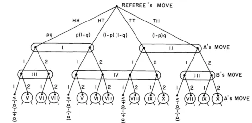
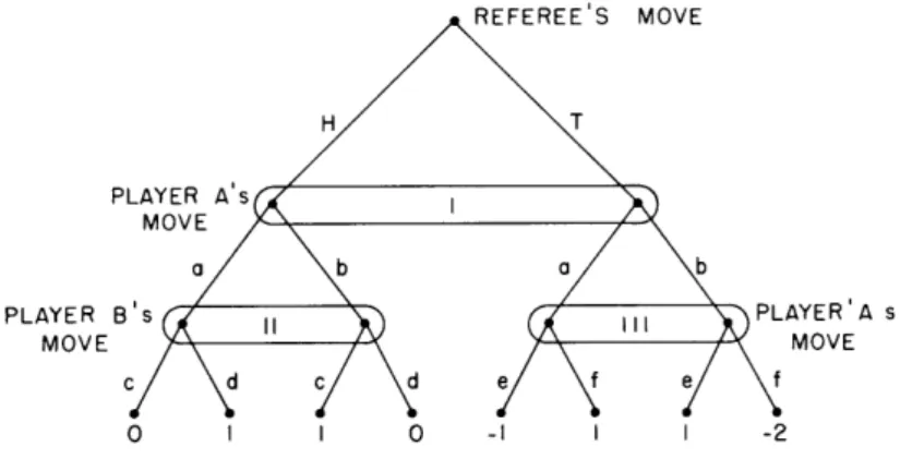
of the company affects the net profit for that year and also the amount of technical knowl-edge gained through research. The last quantity should help the company to increase its future net profits. The game of Kriegspiel is another example of a general adaptive process. Kriegspiel is a modified game of chess in which neither player is allowed to
see his opponent's moves. A referee watches both playing boards and informs players when pieces are captured, or when a player attempts to make a move that is illegal because the path is blocked by a piece of his opponent. A player can learn much about the disposition of his opponent's pieces by attempting to make an illegal move. As a result, both the amount of information a player gathers about the arrangement of pieces and the amount by which the strength of his position changes depend upon his move.
Bush and Mosteller11have developed one of the most widely known general adaptive systems. They made no claims for their "stochastic models for learning" other than that the models are good representations for the outcomes of certain experiments with animals and perhaps can be applied to human behavior. The Bush-Mosteller model sup-poses that the behavior of an organism can be represented at any time by a probability distribution over the courses of action available to the organism. At each trial the response of the organism and the outcome selected by the experimenter determine what event has occurred. Each possible event is associated with a Markov operator that oper-ates on the probability distribution. This produces a new probability distribution that represents the behavior of the system at the next trial. Some organisms that become better at performing certain tasks as they gain experience can be simulated by Bush-Mosteller models. Furthermore, these models can be classified as general adaptive systems (although this was not the intent of their authors' work) because both the data gathered and the reward received at each trial are dependent upon the system's response at that trial. If the parameters are properly chosen, the ratio of the number of success-ful to unsuccesssuccess-ful events increases as the system gathers more data.
Robbins1 2 has posed an interesting problem: "An experimenter has two coins, coin 1 and coin 2, of respective probabilities of coming up heads equal to P = 1 - q and p2
1 - q2 the values of which are unknown to him. He wishes to carry out an infinite sequence of tosses, at each toss using either coin 1 or coin 2, in such a way as to maxi-mize the long-run proportion of heads obtained." (In this paper Robbins gave a good-but not optimum - rule for selecting the coin at each toss. A better rule was suggested by Isbell.1 3 ) A system (experimenter) that performs this maximization is a general adaptive system. The outcome of a toss is dependent upon which coin is tossed, and this outcome determines both the payoff and the data available to the sys-tem.
Several authors have made other excellent contributions to the field of general adap-tive systems: Robbins,14 Flood,15 Bradt, Johnson, and Karlin,16 Kochen and Galanter,17
and Friedberg. 18,19
II. ADAPTIVE DECISION PROCESSES
The mathematical systems that we call adaptive decision processes are general adap-tive systems. They are more restricted than the sequential decision problems posed by Robbins 4; but they represent a fairly broad class of general adaptive systems. It is hoped that the solutions derived for these processes will be a step toward the solution of more general types of sequential decision problems.
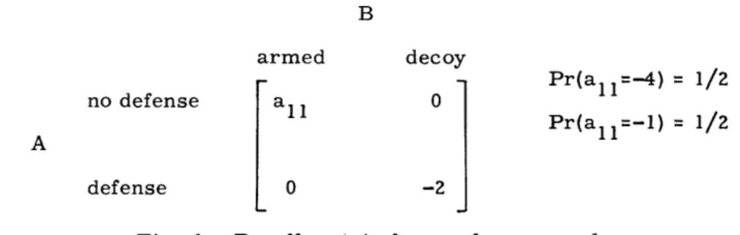
The following warfare situation is a simple example of the type of "realistic n activity represented by adaptive decision processes. The aggressor, called player B, sends missiles toward the defender, called player A. Two indistinguishable types of missile can be sent by B - an armed rocket or a decoy. Player A can use a thoroughly reliable and accurate antimissile missile if he wishes; furthermore, A can tell whether or not a missile sent by B was armed after it has been destroyed or after it has landed in A's territory. The only unknown quantity is the destructive power of B's armed missile when it is allowed to reach its target. Player A has information from two equally reliable spies. One asserts that A will lose one unit (the units may be megabucks) if he allows a warhead to reach his shores; the other spy says the loss will be four units. Player A assigns probability 1/2 to each of these values. However, once A allows an armed mis-sile to land, he will know from then on whether the true destructiveness is 1 or 4. The only other significant loss occurs if A sends an antimissile missile to destroy an unarmed enemy rocket; the loss for this event is 2 units, because of the needless expense. Since A faces the prospect of enduring B's bombardment for a long time, he considers the advisability of learning, by sad experience, the loss that is due to a live missile that is allowed to reach its target. After A has that information, he can decide upon the desirability of using antimissile missiles. In order to make a scientific decision, A constructs the 2 X 2 payoff matrix shown in Fig. 1. The entry in row i and column j,
B armed decoy Pr(all=4) = 1/2 no defense a 0 A11
I
~Pr(a
1ll=-l) = 1/2 A defense 0 -2Fig. 1. Payoff matrix for warfare example.
aij, represents the expected return to A and the expected loss to B is a selects the alternative corresponding to row i and B selects the alternative corresponding to col-umn j. For example, a1 2 equals 0 because A receives no return when he sends no anti-missile anti-missile against a decoy; however, a2 2 equals -2 because A gains -2 units (loses 2 units) and B loses -2 units (gains 2 units) when A sends an antimissile
missile to destroy a decoy.
In this report we present derivations for optimum strategies for player A, based upon certain assumptions about player B. Decision processes in which the payoff matrix is only partially specified at the beginning of an infinite sequence of decisions are studied.
A brief introduction to the theory of games is given in Appendix I. A reader who has no knowledge of the subject will find this introduction adequate to carry him through all but the most detailed of the following arguments. Other references are also sug-gested.2 1 - 5
2. 1 Definition of Adaptive Decision Processes
An adaptive decision process consists of an m X n, two-person, zero-sum game that is to be played an infinite number of times. After each step ("Step" implies a single play of the m X n game.) the payoff is made and each player is told what alternative has been selected by his opponent. The payoff matrix is not completely specified in advance. The nature of the uncertain specification of the matrix and the process by which the uncertainty can be resolved are the heart of adaptive decision processes. Unknown pay-offs are selected initially according to a priori probability distributions, and the players are told only these probability distributions. If a.. is one of the unknown payoffs, the players do not learn the true value of a.. until, at some step of the infinite process, player A (the maximizing player) uses alternative i and player B (the minimizing player) uses alternative j. At this step both players are told the true value of aij, so that it is no longer unknown; A receives aij and B loses aij. Of course, when all of the unknown payoffs have been received, the process is reduced to the repeated play of a conventional m X n, two-person, zero-sum game.
One can visualize a large stack of matrices, each with all of its payoffs permanently recorded. Some of these payoffs are hidden by opaque covers on each matrix. A proba-bility is assigned to each matrix in the stack. The players know this probaproba-bility dis-tribution. One of the matrices is chosen, according to the probability distribution, by
a neutral referee, and that matrix is shown to the players with the opaque covers in place. The game is played repeatedly until the pair of alternatives corresponding to one of the covered payoffs is used. The cover is then removed, and the play resumes until the next cover must be removed, and so on. This process continues until no cover remains. The completely specified game is then repeated indefinitely.
Three basic types of adaptive decision process are discussed in this report. Adaptive Bayes decision is covered in Section III. This case is the situation in which player B is nature, and the probabilities of occurrence of the n states of nature are known and are the same at each step of the process. For example, in the problem illustrated by Fig. 1 if player B announced that half of his missiles were duds, and that there was no corre-lation between the alternatives that he had selected from one step to the next, then A could use the results given in Section III of this report to determine an optimum strategy.
Adaptive decision under uncertainty is discussed in Section V. In this case player A knows nothing about B's strategy. The analysis is based upon the assumption that A uses the same probability distribution over his alternatives at each step of the process until he receives one of the unknown payoffs, after which he changes to another repeated distribution, and so on. Furthermore, A is assumed to adopt the conservative attitude that he should use the strategy that maximizes his return when B selects a strategy that minimizes A's return. Referring to the problem associated with Fig. 1, we see that adaptive decision under uncertainty implies that aggressor B knows both the true loss associated with a hit by an armed missile and also what repeated probability distribution defender A will use. If B always uses this information to minimize A's expected return, then A must select a distribution to maximize the minimum return. Other ways of approaching the problem of adaptive decision under uncertainty are discussed.
A third case, considered in Section IV, covers adaptive competitive decision. Player B is assumed to be an intelligent player attempting to minimize the return to player A. There are two subclasses of adaptive competitive decision: the equal information case, in which A and B are given the same a priori knowledge about the unknown payoffs; and the unequal information case, in which the a priori data are different. The former sub-class corresponds to the situation shown in Fig. 1 when both players make the same evaluation of the probabilities for payoff a1 1; one example of the latter subclass is the
situation in which B knows the true value of all, but A does not. 2.2 Measure of Performance
The phrase "maximize the return" is not precise enough to form a basis for further analysis. It is certainly true that A should play so as to receive a large payoff, learn the payoffs that are unknown to him, and prevent B from learning the payoffs that are unknown to B. Also, A should extract what information he can about the payoffs unknown to him by observing the alternatives that B has chosen during previous steps, and not divulging to B, by the alternatives A chooses, any information about the payoffs unknown to B. It is necessary to find a quantitative measure of performance that will incorporate
all of these aims and then to select a strategy for A that optimizes this measure. The measure that first occurs to us is the expected sum of the payoffs at each step of the game. Player A should attempt to maximize this sum, and player B to minimize it. However, since this measure is generally infinite, the maximization or minimization of the infinite quantity would be meaningless. The difficulty of having to deal with an infinite quantity can be solved by dividing the expected sum of the payoffs for the first N steps by N in order to get the expected payoff per step. The limit of the expected payoff per step can be taken as N approaches infinity. The difficulty with this measure of performance is illustrated by a simple example. Consider two different strategies of player A for which all of the unknown payoffs are learned before the thousandth step of the game and the appropriate minimax strategy of conventional game theory is repeated from the thousandth step on. Both strategies will have the same limit of expected payoff
per step, which is equal to the minimax value of the payoff matrix. Essentially, this is true because in the limit the contribution of the first thousand payoffs is negligible. This measure of performance was rejected because it neglects the effects of the data-gathering process. A measure of performance that does not discriminate among the many strategies for which all the unknown payoffs are learned in a finite number of steps is not useful.
A more useful measure of performance is the expected sum of the discounted payoffs at each step. This measure of performance has been used successfully by Arrow, Harris ' and Marschak,2 6 and by Gillette2 7 for handling infinite processes. The discounted pay-off is especially pertinent to economic situations. For example, if the steps of an adap-tive decision process are made annually and the payoff is invested at 3 per cent interest
(compounded annually), then $100 payoff received now will be worth $103 one year from now. Also $100 received a year from now is equivalent to $100/1.03 invested now. Therefore the present worth of all of the discounted payoffs is the expected sum of the current payoff plus 1/1. 03 times the payoff that will be received a year from now, plus
(1/1. 03)2 times the payoff that will be received two years hence, and so on. The expected sum of the discounted payoffs converges. This measure of performance places more emphasis upon present return than future return. Therefore it overcomes the objection raised against the limit of expected payoff per step. Nevertheless, the possibility exists that with one of two strategies all the unknown payoffs are learned within a finite number of steps, while with the other they are not. Yet the expected sum of the discounted
pay-offs for the former strategy may exceed the sum for the latter strategy for some values of the discounting factor and may be less for other values. This is a reasonable objec-tion to the use of the expected sum of discounted payoffs.
Before some notation is introduced for the purpose of defining the mean loss measure of performance, a basic theorem will be stated explicitly. This theorem states that the players of adaptive decision processes lose no flexibility by restricting their strategies to a class called behavior strategies. A player is said to be using a behavior strategy
if, at each step in an adaptive decision process, he selects a probability distribution over his m (or n) alternatives and uses that distribution to select an alternative. The distribution that he chooses may be dependent upon his knowledge of the history of the process (alternatives selected by both players and payoffs received at all preceding steps). Since behavior strategies are completely general for adaptive decision proc-esses, in the following discussions it will be assumed that players do use behavior strat-egies. This theorem is an obvious extension of Kuhn's results.2 8
Some notation can be introduced. The probability distribution used by player A at the kth step is denoted pk pk k .. Pm), where pk is the probability that A selects alternative i at the kth step. Hence
m
i=l
6
k k k Similarly, the probability distribution used by B at the kth step is denoted q (ql qk
k\ k k "'
., ). Note that k is a superscript -not a power. In general, pk and qk depend upon the past history of the process. The value of the payoff matrix is denoted v; it
rep-resents the maximum expected return that A could guarantee himself (by an appropriate selection of a probability distribution) at one step, if all of the unknown payoffs were uncovered. Of course, v is a function of the values of the unknown payoffs. The precise meaning of the value of v for the three cases of adaptive decision processes will be dis-cussed in the appropriate sections of this report. The expected return to player A at the kt h step, when A uses pk and B uses qk, is denoted rk
m n
rk _ E X piiqj aij. i=l j=l
Since some of the quantities ai. represent unknown payoffs, rk is a function of pk qk and of the values of the unknown payoffs. The term Lk = v - r is called the single-step loss at the kt h step; it is the difference between the expected payoff that A could guaran-tee himself if the values of the unknown payoffs were known and the expected payoff A does receive. If the limit as N approaches infinity of the sum of single step losses for the first k steps exists, it is called the total loss L. The values +oo and -0o are allowable limits.
00
L= Lk
k=l
The expected value of the total loss L, with respect to the probability distributions for the unknown payoffs, is called the mean loss. It is denoted
L= L(unknown payoffs) dP(unknown payoffs),
where P(unknown payoffs) denotes the cumulative probability distribution function for the unknown payoffs. The derivations of the mean loss for the three cases of adaptive
deci-sion will also be covered.
The single-step loss, Lk , represents the expected loss to A at the kt h step because of his lack of data for the unknown payoffs. Lk is similar to the "regret" or "loss" func-tion defined by Savage,2 9 except that regret is defined as the difference between what a player could receive if he knew his opponent's choice of alternative, and what he does receive. Lk is the loss for a single step of the game. When the losses for all of the
steps are summed, the total is L, which is a function of the values of the unknown pay-offs and p , q p , q2 L is the total loss that A sustains because of his igno-rance of the true values of the unknown payoffs. L, the expected value of L (with respect to the probability distributions for the unknown payoffs), is the measure of performance used in this report.
7
-Player A should play so as to minimize the mean loss L; whereas, B should play to maximize this quantity. If A plays wisely, Lk will be smaller, in general, than if
he plays foolishly, and as a result L will also be smaller. Two other factors suggest that the mean loss is a good measure of performance. First, it will be demonstrated that there exist strategies for the players that make finite. Second, if we consider
the definitions for L and L applied to an N-truncated adaptive decision process (a proc-ess that terminates after N steps), we arrive at conclusions that seem reasonable. The following relationships are clearly true:
N LN Nv - rk k= 1 N LNv Nv- rk, k=l kk 1
where LN is the total loss, and LN v, and rk are the mean values of LN, v, and rk respectively. Since V is not dependent upon the strategies used, the mean N-truncated loss, LN, is minimized when player A maximizes the expected sum of his returns at the first N steps, and LN is maximized when B minimizes that sum. Hence, by using the mean N-truncated loss measure of performance, we arrive at the same optimum strategies for A and B as we would when we apply the measure of performance that was
suggested first to the truncated process (the expected sum of the payoff at each step). Note that assumptions of linear utility preference, independence of utility with time and absence of intrapersonal variations in utility, have been tacitly made. They enter implicitly into the definition of the mean loss.
2. 3 Summary of Results
Through adaptive Bayes decision it has been demonstrated that an optimum strategy for player A consists of the repeated use of one probability distribution over A's alter-natives until one of the unknown payoffs is received, and then the use of another distribu-tion until another payoff is received, and so on, until all of the payoffs are known. Then A must repeat another probability distribution indefinitely. Such a procedure is called a stationary strategy. The probability distributions in the optimum piecewise-stationary strategy assign probability 1 to one of A's alternatives and 0 to the others. In general, A should attempt to learn the unknown payoffs as soon as possible. A tech-nique is presented for reducing the computational effort required to determine the opti-mum piecewise-stationary strategy. This simple method eliminates a large amount of computation.
The analysis of adaptive decision under uncertainty is based upon the assumption that player A uses a piecewise-stationary strategy. The significant result is that A can guarantee that the mean loss is finite if he selects a probability distribution that lies
inside a certain linear constraint space, That is, if the components, P1, p2, ... , P of the p vector satisfy a given set of linear inequalities, then L must be finite. When only one payoff is unknown, the optimum p vector is calculated by a simple algorithm. No simple rule has been derived for the case in which there are two or more unknown payoffs.
The principal results for adaptive competitive decision are: (a) a minimax solution exists for the case in which there is equal information, and piecewise-stationary strate-gies are optimum for both players; and (b) in general, piecewise-stationary stratestrate-gies are not optimum for unequal information. A straightforward technique for computing the minimax strategies in problems of equal information will be developed in Section V, but no solution is available for the unequal information case. Another result demon-strates that competitive processes with unequal information can be given meaning as infinite game theory problems.
9
III. ADAPTIVE BAYES DECISION
If player B uses the same probability distribution at each step of the decision proc-ess, and if the alternatives are selected independently at each step, then B is said to be using a stationary strategy. In the adaptive Bayes decision process player B is assumed to use a stationary strategy, which is known to player A. This corresponds to situations in which the alternatives of player B represent possible states of nature, the probability distribution over the states of nature is known, and the state of nature is independently determined at each step of the process. The payoff a.. represents the
1J
award to player A when he uses alternative i and state of nature j occurs. An example of the situation illustrated by Fig. 1 would be a problem of adaptive Bayes decision if the defender (player A) learned through his spies that the aggressor intended to send a certain fraction, ql, of his missiles with warheads and q2 = 1 - ql without warheads.
It is also assumed that none of B's alternatives occurs with zero probability: qj> 0 for j = 1,...,n.
This eliminates from consideration extraneous columns of the payoff matrix.
It is demonstrated in Appendix II that the piecewise-stationary strategy for which the mean loss is smallest is actually the optimum strategy
min L(S') = min L(S),
where S' represents the class of all piecewise-stationary strategies, and S is the class of all possible strategies. This result is the one that intuition leads us to expect. Since no new data are gathered until one of the unknown payoffs is received, it does not seem likely that the probability distribution for each step of the optimum strategy should change between the times when unknown payoffs are learned. The reader is advised to defer the reading of Appendix II until he has read section 3. 1. The result given in Appen-dix II, however, is used hereafter.
3. 1 Single Unknown Payoff
The value, v, of the payoff matrix in the adaptive Bayes decision process represents the largest expected return that A could guarantee himself, for a single step of the proc-ess, if he knew the true values of the unknown payoffs
m n m n
v max( I piqjai) max Pi qi (1)
P i=l j=1 P i=l j=l
where p represents the set of all probability distributions over the alternatives of A. The expected return when alternative i is used will be denoted
n
E(row i) = E qjaij . j=l
When the notation E(row i) is used in Eq. 1, we have m
v = max Pi E(row i) = max E(row i) (i= 1).
P i=l i
The case for a single unknown payoff is considered first. It is completely general, in order to let a11 be the unknown payoff. The single-step loss at the first step and
1
at each succeeding step, until a1 is received, is L = v - r. Because of the stationari-ness of the strategies of A and B, it is true that
1 2 3
P=P =P =p =...
1 2 3
q=q =q q =
until al11 is received. Therefore, no superscript is applied to the expected return, r. After a11 is received, A is assumed to use an optimum strategy for the succeeding steps of the process. This is a fundamental assumption that will be used many times in this report. In general, for the purpose of calculating optimum strategies at any step of an adaptive process, the assumption is made that the players use optimum strategies for the process that remains after the next unknown is discovered. This assumption may be made only for situations in which the techniques of finding the optimum strategies have been developed. Once a11 is discovered, A has all the data available to determine the alternative(s) for which the expected return equals the value of the payoff matrix. As a result, by repeatedly using an optimum alternative, A can play so that the single
-step loss is zero after a1 is received. It follows that
Lk (1Plql)k- L1
because the single-step loss at the kt h step equals the probability that al l is not dis-covered before the kth step [(l-plql)k- l] times the single-step loss when all is not known [L1] (plus the probability that all is discovered before the kth step times the single-step loss when a11 is known, which equals zero). Therefore, the total loss is
oo o00
L= L k= (-plq I)k- lL,
k=l k=l
and the mean loss is
oo
L = (1-plql)k 1 L1, (2)
k= 1
where L1 is the mean value of Ll(all) with respect to the unknown payoff. If P(all) is the cumulative probability distribution function of unknown payoff all' then
Lo SLl(all) dP(a I1).
The single-step loss L1 is non-negative for all possible values of all and all distribu-tions P because the value v of the payoff matrix represents the maximum value of r.
Consequently, L is always non-negative. As a result, L exists and is a non-negative number or +oo.
It may be possible to select a distribution, p, for which L equals zero. This is true if r = v for all possible values of all; that is, if
m
Pi E(row i) = max E(row i) i
for all possible values of a 11 ' This is equivalent to stating that there exists an
alter-native i for which E(row io) > E(row i) for all possible values of al 1and all i i io . This is true if either of these cases holds:
(a) Emin(row 1) > E(row i) for all i 1.
(b) E(row io) > Emax(row 1), and E(row io) >E(row i) for all i 1 or io.
E max(row 1) and Emin (row 1) denote, respectively, the maximum and minimum possible values of E(row 1):
n Emax(row 1)= qlall max + qja1j
j=2 n
Emin(row 1)= qal1 min + qjalj, j=2
where a11 max and a1 mi are, respectively, the maximum and minimum possible val-ues of all. If we introduce the following notation, the results just derived can be expressed more concisely:
n
E(row 1) ql SalldP(all) + qjalj
j=z
If case (a) holds, V = E(row 1). Thus L equals zero if A uses alternative 1 repeatedly. If case (b) holds, = E(row io), so L equals zero if A uses alternative i repeatedly. Case (a) implies that the expected return for alternative 1 is at least as large as the expected return for any other alternative, irrespective of the true value of a1 1; case
(b) implies that the expected return for alternative i is at least as large as the expected return for any other alternative, irrespective of the true value of a 1'
12
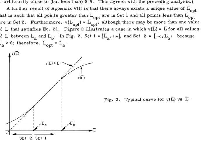
:·~~~~~~~~~~~~~~~~~~~~~~~~~~~~~~~~~~~~-Once the cases for which = have been dealt with, it is possible to con-sider the remaining cases, for which > . (The quantity T is the mean value of r:
= f r(a dP(all ll) ) plql fa 11 dP(all) + Z piq.a..) Equation 2 implies that
v-rM
(3) p1q1
It is demonstrated in Appendix III that r assumes its minimum value for some P1q1
distribution, p, with one component equal to 1 and the remaining components equal to 0; therefore, Eq. 4 follows from Eq. 3.
-min - r minv min - E(row 1) - E(row 2) - E(row m)
P p p q q1 0 0
(4) Because V > T for all distributions p and because ql > 0, it follows that
L V - E(row 1)
min q1
The optimum strategy for A is to use alternative 1 repeatedly. All of the preceding results can be summarized by saying that
0 if V = E(row io) for any io 2, . .,m Lmin = V - E(row 1)
q otherwise.
Therefore, the minimum mean loss, Lmin, is bounded if all positive payoffs are boun-ded. If a distribution, p, with its it h component, Pi, equal to one is denoted by ei, then we can say
ei0 if V = E(row io) for any io = 2,...,m Popt =
el otherwise.
The meaning of this result is clear. The logic behind the cases in which V = E(row i) or V = E(row 1) has been discussed already. The mean loss is 0, for in these cases player A has no reason to wish to know a1 1, since no matter what value the unknown assumes, alternative i dominates all others. Therefore, A's strategy involves no attempt to learn the true value of a11' However, in the case for which there is no uniformly best alter-native, A's optimum strategy is to use alternative 1 repeatedly (in order to discover the true value of unknown payoff all as soon as possible), and after a1 has been received to use an optimum alternative repeatedly for the conventional Bayes decision process that results. In this case the mean loss equals the mean single-step loss,
13
I
L = V- E(row 1) > 0,
times the expected number of steps before all is discovered, which is 1/q1.
If q = (1/2, 1/2) for the missile defense problem of Fig. 1, the following quantities are easily calculated:
-2 if -4 -1 if a -4
E(row 1) /2 if a -1,
v(a
1)-1/2 if all -1,/2 if a
E(row 2) = -1.
The preceding analysis indicates that Lmin equals +1: -3/4 - (-5/4)
mm 1/2
A's optimum strategy is to use alternative 1 repeatedly until all is received, after which he should use alternative repeatedly if all = { -14
3.2 Multiple Unknown Payoffs
The following discussion is for the purpose of determining the optimum probability distribution, Popt' for the first segment of A's optimum piecewise-stationary strategy when two payoffs, a1 1 and a2 2, are unknown. The special cases in which both unknown payoffs are in the same row or column of the payoff matrix will also be mentioned. After one step of the process has occurred, either a 1 has been received (with probability p1ql), a2 2 has been received (with probability p2q2) or neither has been received (with probability (1-p 1ql-p 2q 2)). Player A can play in an optimum fashion after he has dis-covered a 1 or a22' since the optimum strategy for cases with a single unknown payoff has been derived. Let the total loss sustained by A if he uses the optimum strategy for the process with a single unknown payoff, a2 2, be denoted Lmin all. The optimum strategy is a function of the value of a1 ; therefore Lmin a1 1 is a function of both all and a2 2. Lmin la2 2 is defined analogously.
Since player A uses a piecewise-stationary strategy, the single-step loss at each step is L1 until all or a22 is received, after which the loss is Lmin lall or Lminla22. Therefore, the total loss is
+ ( 1-P1q1-P2q2) [ L +PlqLmin la1l +P2q2Lmin la2 2 + (l-pll-P 2q2)[L1+
...
]](L +plqlminlal +p2q2Lmin a22) (1 -p1q1P2q2)k; (5)
k=O
14
and the mean loss is
00
L Z(iO~p q L 1,111p~q'2)E (\ -k (6)
k=O where
L~mla~ -(a ) dP(a )
Lmin I a 1 Lmin(a 1 1
Lmin(all) is the minimum mean loss for the process with a single unknown payoff a2 2,
as a function of a11 ' Lmin la22 is defined similarly.
It may be possible to select a distribution, p, for which the mean loss, L, equals zero. Because L Lmin al, and Lmin a2 2 are non-negative for all possible values of the unknown payoffs and for all distributions, Eq. 6 implies that the mean loss is zero if and only if L1 la Lmin la22 = 0. The mean single-step loss, L1, equals zero when r = v for all possible values of (al 1' a2 2); that restriction also implies that both Lmin all and Lmin la2 2 equal zero. Conditions (similar to cases (a) and (b) for the single unknown payoff process) that must be satisfied if the preceding restriction is to hold, are easily derived. These are cases in which V equals E(row i ), E(row 1), or E(row 2). Player A has no need to learn the true values of the unknown payoffs. If these cases are eliminated first, then the situation in which L1 is positive may be handled. Equation 6 leads to the following expression for the mean loss.
L1 + PlqLmin lall + p2qLminla2 2 L
Plql + P2q2
A result of Appendix III implies that L assumes its minimum value for some distribution = ei
Lm
.< -E (r w 1) + qminl V(row 2) + q2Lminla 2 2
mm ql q2
V - E(row 3) v - E(row m)
0(rw
) 0qlminlaIf V > F for all p, the following relation is true:
min[V-E(row 1)+qmini la V-E(row 2)+ qzLmin az]
min q1 q2
where the definition of E(row 2) is similar to that of E(row 1). All of the preceding results can be summarized in the following form:
15
----il-0 if = E(row i ) for any io = 3 . .. ,m
minv -E(row 1) + qLminal v - E(row 2) + q2Lminla2 otherwise
mn ' q2 otherwise
(Lmin is bounded if all possible payoffs are bounded.) ei if v = E(row i) for any i = 3...,m
0
P opt - e v - E(row 1) + qlLmin all <V - E(row 2) + q2Lmin a 22
1 otherwise, if 1 q2
e2 otherwise.
Once again, the solution shows that the optimum strategy for player A is to use alternative 1 or 2 repeatedly in order to find out unknown payoff a 1 or a22 as soon as possible, unless the expected return of row i is greater than the expected returns for all of the other rows, irrespective of the true values of a11 and a22. (In the last case, A is not interested in learning the true values of al l and a2 2, so he uses alternative i repeatedly.) After A learns the value of a11 or a22, he should use the optimum strat-egy for the process with a single unknown payoff that remains.
We may ask the questions: If player A must learn both a11 and a22 eventually, what difference does it make which he tries to learn first? Why should there be any difference between the mean losses when we use p = e or p = e2? These questions are answered with the help of the mathematical manipulation included in Appendix IV. The results in Appendix IV may enable player A to determine his optimum strategy by means of very simple calculations. This method of determining Pp t is called the abbreviated method, and is valid when a11 and a22 are statistically independent. Three possible situations can arise:
(i) E max(row 1) > E max(row 2) (ii) Emax(row 1) < E max(row 2) (iii) Emax(row 1) = Emax(row 2).
In the first case, the optimum strategy for A is to use p = e1. The reason is that when player A uses e and discovers the true value of all, it is possible that E(row 1) E max(row 2). (The expected return for alternative 1 is at least as large as the expected return for alternative 2 - irrespective of the true value of a2 2.) Thus, after discovering all, A may never wish to learn the true value of a22. On the other hand, if player A starts the two-unknown payoff process by using e2, he must always learn al l after he discovers the true value of unknown payoff a2 2 because it is impossible, by the definition
16
of case (i), to find that E(row 2) > Emax(row 1) for any value of a22. Therefore, if A must always use e1 at some part of his piecewise-stationary strategy until he discovers
al 1 his optimum strategy is to do this first and then use e2 only if it is necessary. In case (i) it is not true that A "must" learn both all and a22 eventually. In case (ii) Popt e2; analogous reasoning demonstrates the validity of this result.
There are four subcases of case (iii)
(a) Pr(a11=all max = 0, and Pr(a22 a22 ma x 0, (b) Pr(a1 1=a l l max) > 0, and Pr(a2 2 a2 2 max) 0 (c) Pr(all a l l max) 0, and Pr(a2 2=a2 2 max) > 0' (d) Pr(a1 1=a l11 max) > 0, and Pr(a2 2=a2 2 max)> 0.
Subcase (a) is the situation in which the random variables a1 1 and a2 2 have probability distribution functions with probability zero of actually attaining the maximum values,
or else they have infinite maxima. The solution for subcase (a), according to the results of Appendix IV, is that the mean losses resulting from the use of distribution e1 or e2 first are the same, so both strategies are equally optimum. The reason is that after learning all, it will be necessary with probability one for A to learn a22 in order to discover the optimum strategy for the payoff matrix, and vice versa. The solution for subcase (b) states that Popt = el', since if e2 is used first, it will be necessary with probability one to use p = e1 to discover al; however, if e1 is used first, it will be necessary only with probability Pr(al 1 < all max) to use e2 in order to discover a2. Subcase (c) is the converse of subcase (b): Popt = e2' Subcase (d) is not as simple as the others, and involves the comparison of the following expressions:
E max(row 1) - E(row 1)
ql Pr(a22=a22 max)'
E (row 2) - E(row 2)
mx q2 Pr(al l=al 1 max)
If the former is smaller, Popt = e; if the latter is smaller, Popt = e2; if the two terms are equal, both e1and e2are optimum. It is difficult to read any significance into this result. Because of the abbreviated method it is possible to derive the optimum strategy from a few easily calculated quantities. An example is worked out in Appendix V by both the regular and abbreviated methods, to illustrate the concepts just derived. This example is a dramatic demonstration of the power of the abbreviated method.
The special cases in which the two unknown payoffs are in the same row or column must be considered now. If the unknown payoffs are in the same column, the preceding results apply with extremely minor modifications. It is obvious that the preceding results can also be specialized to handle the case in which both unknown payoffs are in
17
the same row. Assume that al and a12 are not known. Some simple manipulations lead to the following conclusions:
0 if = E(row io) for any i = 2, ... ,m
min
V - E(row 1) + qLminlall + qLminla12 otherwise otherwise q + q2
and
Sei if V = E(row io) for any io = 2, ... ,m Popt =
He 1 otherwise.
The case with three unknown payoffs, all, a2 2, and a3 3, is handled just as the case of two unknown payoffs:
O if = E(row i) for any i = 4,...,m
Lmin V - E(row i) + qiLmin aii
i=, 2, 3 t qi
qi
min
11
otherwise.Here, for example, L min = in(all) dP(all), and Lmi (all) is the minimum mean loss for the case with the two unknown payoffs a22 and a33 as a function of a 11
The reader will appreciate the difficulties in notation that arise when an attempt is made to write a general expression for cases of more than two unknown payoffs with all possible locations of the unknown payoffs taken into account. Nevertheless, the prin-ciples that have been described are still valid for more than two unknown payoffs. A general principle that deserves attention is that Lmin is bounded whenever all possible payoffs are bounded.
Algorithms that take into account all possible situations that arise can be constructed for the purpose of machine computation of optimum strategies. The computations for k unknown payoffs depend upon computations for the k cases of k-I unknown payoffs, each of which, in turn, depends upon the k-i calculations for processes with k-2 unknown payoffs, and so on. The reader who has ventured into Appendix V will realize how very rapidly the magnitude of the computational effort grows with the number of unknown pay-off s.
It is regrettable that the complexity of the calculations for three or more statistically independent unknown payoffs prevents an extension of the type of analysis for the abbre-viated method which was performed in Appendix IV with two statistically independent unknown payoffs. Nevertheless, the arguments presented above in support of the
analytic results are valid, so the abbreviated method can be extended to the cases in which there are more than two independent unknown payoffs. The essence of the method is, first, to check for the cases in which V = E(row i) or V = E(row i) and for the cases in which the minimum expected return for some alternative exceeds the maximum expected return for another alternative. After these situations are dealt with in the appropriate manners (if V = E(row i) or V = E(row i), Popt = ei; if alternative i is domi-nated, eliminate it from consideration), a comparison is made of E max(row i) for all alternatives associated with unknown payoffs. If there is a single maximum term, then Popt = ei' where i is the index of the maximum alternative. If the maximum is assumed for two or more alternatives but the probability is zero that the expected return for any of these alternatives assumes its maximum value, then Popt = ei' where i corresponds to any one of the maximum alternatives. The case in which several alternatives have the same maximum value of expected return but only one has a finite probability of assuming the maximum implies that Popt = ei i corresponding to the unique row. Because the few remaining cases have proved too complex to understand, it is necessary to return to the standard method in order to calculate the optimum strategies when sev-eral alternatives have positive probability of assuming the same maximum value of expected return.
19
IV. ADAPTIVE DECISION UNDER UNCERTAINTY
4. 1 The Meaning of Adaptive Decision Under Uncertainty
When player A is making decisions in the face of uncertainty, he knows that at any step of the decision process one of n states of nature exists. The uncertainty about which one exists, and the uncertainty about the process that selects the state of nature
are the problems player A must face. If the probability distribution of the states of nature is stationary, and if A knows what this distribution is, he should use the optimum
strategies developed in Section III for adaptive Bayes decision processes. Under other circumstances he must resort to different techniques.
If nature uses a stationary strategy but A does not know the repeated distribution, he is forced to make some assumption that will make the problem amenable to solution. The validity of the assumption depends upon the nature of the process. For example, A may assume the existence of an a priori probability distribution over the possible probability distributions of nature 's stationary strategy. (A common a priori distribu-tion is the one for which all of nature's distribudistribu-tions are equally likely.) After each step of the process player A can derive an a posteriori probability distribution of nature's distributions, which is a function of the a priori distribution and the alternative used by nature. When A has learned all of the unknown payoffs, his problem is not com-pletely solved. Because he does not know B's strategy, he does not know which of his own strategies is optimum. The problem A faces when all of the payoffs are known is an example of a special adaptive process, since the information gathered about B's strat-egy is independent of A's stratstrat-egy. The problem is a generalization of a problem dis-cussed by White.7 The optimum strategy for player A is to use, at each step, the alternative for which the expected return, at that step, is maximized. The correct alternative is easily determined. The problem that A faces before he knows the entire payoff matrix is a general adaptive process, since the information that he gains about the unknown payoffs depends upon the alternative he selects, so the interesting question is, How should A play when some payoffs are unknown? The mean-loss measure of performance can be applied to this form of the adaptive decision under uncertainty prob-lem. A reasonable definition for v, the value of the payoff matrix, is the expected return player A could guarantee himself if he knew both the true values of the unknown payoffs and the distribution used by nature. In this case the single-step loss does not equal zero when all of the payoffs are known, as it does in the adaptive Bayes decision process. Since it is not known whether the mean loss can be finite for any strategy of A, it may be necessary to use a different measure of performance.
Player A faces a more difficult task when it is not reasonable to assume an a priori distribution for the distribution of nature's stationary strategy. It must be realized that the simpler problem of how to play a game against nature when nature 's strategy is unknown - but all the payoffs are known - has not been solved yet. One conservative
20
approach advises player A to use the minimax distribution for the payoff matrix repeatedly. This strategy guarantees A an expected return of at least v at each step. Another approach advises A to make use of his knowledge of the alternatives selected
by nature at preceding steps in order to estimate nature's strategy. A paper by Hannon3 0 deals with this technique. However, there is no generally accepted solution to the prob-lem. Because of the difficulty in finding a satisfactory solution for the special adaptive
process under uncertainty when all of the payoffs are known, the general adaptive proc-ess of repeated decision under uncertainty when some payoffs are unknown appears to be a monumental problem.
When the assumption that nature uses a stationary strategy is not valid, the problem is even more difficult. A very cautious approach suggests that A assume that nature's strategy is chosen to maximize A's loss. That is, whatever strategy A uses, nature selects the worst (from A's viewpoint) possible strategy. Therefore, A should select a strategy that will minimize the maximum loss. Then he can guarantee that his loss never exceeds the minimax value, irrespective of the actual strategy used by nature. (Because this is an infinite process, the minimax loss does not necessarily equal the maximin loss.) The problem handled in sections 4. 2 and 4. 3 is closely related to the minimax formulation. The true minimax problem is a problem of adaptive competitive decision with unequal information - the case in which player B knows all the payoffs. The general solution for this problem has not been found; the problem discussed in sec-tions 4. 2 and 4. 3 is the minimax solution when player A is restricted to the use of piecewise-stationary strategies. Player B is assumed to use the strategy that maxi-mizes the total loss; this maximizing strategy is a function of both the true values of the unknown payoffs and A's strategy. Player A's optimum piecewise-stationary strat-egy is the one that minimizes the mean value of the maximum total loss.
The calculation of minimum mean loss to be given presently is an upper bound to the loss sustained by player A in problems of adaptive competitive decision with unequal information. If A uses a better strategy than the optimum piecewise-stationary strategy, the mean loss will be smaller than the quantity calculated here; however, the strategy derived below will be a fairly good mode of play for both the problem of competitive decision and adaptive decision under uncertainty. Furthermore, some very interesting concepts are brought to light by this study.
The problem of Fig. 1 represents a case of decision under uncertainty if it is known that the aggressor sends only live missiles, but the warheads are unreliable and may or may not explode. Player B is assumed to be a capricious gremlin who determines whether each missile will explode. The first alternative of B represents explosion; the second alternative, nonexplosion. (The payoffs in Fig. 1 ought to be modified in order to take into account the cost to B of armed missiles that fail; however, the purposes of this exposition will not be furthered by a change in Fig. 1.) Player A, being very cautious, assumes that the gremlin knows both the piecewise-stationary strategy that A will use and the true value of all, and will use this information to maximize A's total
21
loss. Therefore, A should select a strategy that minimizes the mean value of the max-imum total loss.
4. 2 Single Unknown Payoff
The value of the payoff matrix, v, represents the largest expected return player A can guarantee for one step of the process when the payoff matrix is completely known. Since it is assumed that B selects a strategy to minimize the return, v equals the mini-max value of the payoff matrix, which is a function of the unknown payoffs:
m n m n
v max m piqiaij = in max
7
piqjaij p q =l j=l P i=lj=Assume that only payoff al11 is not known. Because A is assumed to use a piecewise-stationary strategy known to B, it can be shown that player B maximizes the total loss by using his optimum piecewise-stationary strategy. The arguments of Appendix II apply almost directly to this case. Because both players are assumed to use the minimax dis-tributions repeatedly after payoff a11 has been received, the single-step loss equals zero after that step. This result allows us to prove that to every nonstationary strategy of B there corresponds a memoryless sequence of distributions for which the total loss to player A is no smaller than the loss for the nonstationary strategy. The total loss
can be written
00 k-1
L=
7
(v-r) ( I-Plqtl),k= t=O
where 1 - plql is defined to be equal to one. No matter what probability distribution A uses, B can select a distribution for which the single-step loss is non-negative; there-fore, the least upper bound to the total loss, with respect to B's strategies, is
non-negative. Let the least upper bound of L be denoted Lo. If Lo = 0, player B can attain a total loss of zero by using a stationary strategy. If 0 < Lo < +oo, the logic of Appen-dix II can be used to show that the optimum piecewise-stationary strategy for B ensures a total loss of Lo. It is easily shown that if Lo = +oo, B can attain a total loss of +oo by using a stationary strategy.
It is possible, therefore, to write an expression for the total loss as a function of the piecewise-stationary strategies of A and B (and of all):
oo
L = (1-plql)k-l(v-r). (7)
k= 1
Three cases can arise:
(a) the maximum value of v-r (with respect to q) equals zero; (b) the maximum value of v-r is positive, and P1 = 0; and
22
(c) the maximum value of v - r is positive, and P > 0.
In case (a), L = when B sets q = ej for any j for which E(col j) = v. At least one such alternative j exists. Then the maximum total loss equals zero. The quantity E(col j)
represents the expected return when B selects alternative j: m
E(col j) A Piaij. i=l
In case (b), L = +oo if B sets q = e for any j for which v > E(col j). There must be at least one such alternative. The maximum total loss for case (c) must be positive. This expression for the total loss follows from Eq. 7:
v-r
[vr- if v r
L= pq Pif (8)
0 if v = r.
In Appendix III it is shown that an expression of the form (v-r)/p lql assumes its maxi-mum value with respect to q when q = e for some j = 1, ... , n. If the largest of the n terms equals a positive number c and occurs for q = e with j 1, and if v = E(col j), then
v-r 0 max v =
q Plql
But Eq. 8 implies that L = 0 when v = r. This difficulty can be avoided if B chooses q close - but not equal - to e., so that L is as close to c as desired. Therefore, it is
J possible to write
L
max L max v-E(col 1) v-E(col 2) v-E(col n)
Lmax axL max P ' 0
q
L
(This expression is admittedly meaningless and is to be accepted only as a convenient notation for the preceding description of the quantity L ma.) Notice that cases a and bmax
are also included in the notation of Eq. 9 for Lmax'
Because Lmax is non-negative for all possible values of p and all ' the mean loss,
L(p) -- Lmax(p, al 1 ) dP(al 1)'
is infinite if Lmax = +oo for any values of a 1that have finite probability. In order to ensure that L(p) is finite, A must select p so that the following relations are satisfied for all possible values of all:
E(col 1) >-v if P1 = 0
E(col j) >-v for j = 2, ... ,n.
These inequalities follow from Eq. 9. If they are satisfied for the largest possible value of v, they are satisfied for all other possible values. Since v is a monotonic, non-decreasing function of a1 1, it assumes its maximum possible value, vmax, when the unknown payoff assumes its maximum possible value, all vmax ' (all max Therefore, A guarantees that L(p) is finite if he selects a probability distribution, p, that satisfies these inequalities:
m
a) Piaij > vmax for j = 2, .. ,n, i=l m b) Piail >1 vmax if P1 = (10) i=1 m C) Pi = 1 i=l d) Pi > 0 for all i = 1, ... ,m.
This is an important result. No matter what piecewise-stationary strategy A selects, and no matter what value the unknown payoff assumes, player B can select a
piecewise-stationary strategy (that depends upon p and a1 ) for which the total loss is non-negative. If A uses a distribution p that does not satisfy inequalities (10a), then the expected return for some alternative j 1 of player B is less than the value of the payoff matrix for some possible value(s) of al 1' B's optimum strategy for that value(s) is to select alternative j repeatedly. In this case the single step loss is positive at each step:
L =v - E(col j) > 0 for k = 1, 2, ....
Because j 1, player A never learns the true value of the unknown payoff. As a result, the total loss is infinite, so the mean loss is infinite also. If inequality (10b) is not
satisfied, then for some possible value(s) of a1 1
Lk =v - E(col 1) > 0 for k = 1,2,....
if B selects alternative 1 repeatedly. Because A never receives a11 when P1 = 0, the total loss and the mean loss are infinite. Relationships (10c) and (10d) are the restric-tions imposed by the fact that p is a probability distribution.
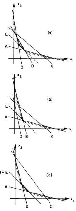
Inequalities (10a), (10c) and (10d) describe a closed convex polyhedron in m space. The coordinates of this m space are P1, ... , m. (Actually, the inequalities determine a closed convex polygon in one hyperplane of m space.) This polyhedron will be called a constraint space for player A.
There exists at least one distribution that lies in the constraint space. Let a11 max