Publisher’s version / Version de l'éditeur:
Evolutionary Computation (CEC), 2011 IEEE Congress on, pp. 1589-1596,
2011-06-08
READ THESE TERMS AND CONDITIONS CAREFULLY BEFORE USING THIS WEBSITE. https://nrc-publications.canada.ca/eng/copyright
Vous avez des questions? Nous pouvons vous aider. Pour communiquer directement avec un auteur, consultez la première page de la revue dans laquelle son article a été publié afin de trouver ses coordonnées. Si vous n’arrivez pas à les repérer, communiquez avec nous à [email protected].
Questions? Contact the NRC Publications Archive team at
[email protected]. If you wish to email the authors directly, please see the first page of the publication for their contact information.
NRC Publications Archive
Archives des publications du CNRC
This publication could be one of several versions: author’s original, accepted manuscript or the publisher’s version. / La version de cette publication peut être l’une des suivantes : la version prépublication de l’auteur, la version acceptée du manuscrit ou la version de l’éditeur.
For the publisher’s version, please access the DOI link below./ Pour consulter la version de l’éditeur, utilisez le lien DOI ci-dessous.
https://doi.org/10.1109/CEC.2011.5949805
Access and use of this website and the material on it are subject to the Terms and Conditions set forth at
Evolutionary computation methods for helicopter loads estimation
Valdés, Julio J.; Cheung, Catherine; Wang, Weichao
https://publications-cnrc.canada.ca/fra/droits
L’accès à ce site Web et l’utilisation de son contenu sont assujettis aux conditions présentées dans le site LISEZ CES CONDITIONS ATTENTIVEMENT AVANT D’UTILISER CE SITE WEB.
NRC Publications Record / Notice d'Archives des publications de CNRC:
https://nrc-publications.canada.ca/eng/view/object/?id=01c32fe6-0056-4670-aafc-94022f56c83f https://publications-cnrc.canada.ca/fra/voir/objet/?id=01c32fe6-0056-4670-aafc-94022f56c83fEvolutionary Computation Methods for Helicopter
Loads Estimation
Julio J. Vald´es, Senior Member, IEEE
National Research Council Canada Institute for Information TechnologyOttawa, Canada
Email: [email protected]
Catherine Cheung
National Research Council CanadaInstitute for Aerospace Research Ottawa, Canada
Email: [email protected]
Weichao Wang
National Research Council Canada Institute for Aerospace Research
Ottawa, Canada
Email: [email protected]
Abstract—The accurate estimation of component loads in a helicopter is an important goal for life cycle management and life extension efforts. This paper explores the use of evolutionary computational methods to help estimate some of these helicopter dynamic loads. Thirty standard time-dependent flight state and control system parameters were used to construct a set of 180 input variables to estimate the main rotor blade normal bending during forward level flight at full speed. Evolution-ary computation methods (single and multi-objective genetic algorithms) optimizing residual variance, gradient, and number of predictor variables were employed to find subsets of the input variables with modeling potential. Clustering was used for composing a statistically representative training set. Machine learning techniques were applied for prediction of the main rotor blade normal bending involving neural networks, model trees (black and white box techniques) and their ensemble models. The results from this work demonstrate that reasonably accurate models for predicting component loads can be obtained using smaller subsets of predictor variables found by evolutionary-computation based approaches.
I. INTRODUCTION
Operational requirements are significantly expanding the role of military helicopter fleets in many countries. This expan-sion has resulted in helicopters flying misexpan-sions that are beyond the design usage spectrum. Due to this change in usage, there is a need to monitor individual aircraft usage to compare with the original design usage spectrum in order to more accurately determine the life of critical components. One of the key elements to tracking individual aircraft usage and calculating component retirement times is accurate determination of the component loads.
The rotor system components and attachments are some of the most fatigue-critical structural components on a he-licopter. Direct measurement of the dynamic loads in these areas has traditionally been accomplished through slip rings or telemetry systems, however, these techniques are difficult to implement and are often unreliable. While advances in sensor technologies in the past decade have produced compact, lightweight, and economical devices, high equipment costs and large data storage requirements still make direct load monitoring impractical.
This work was supported in part by Defence Research and Development Canada (13ph13). Access to the data was granted by the Defence Science and Technology Organisation.
Much research has been carried out using machine learning methods to model operational loads experienced by fixed-wing aircraft structure [19], [7]. In the case of rotary-fixed-wing aircraft, the loading spectrum experienced by the airframe structure is significantly more complex since the dynamic rotating components operate at frequencies several orders of magnitude higher than for fixed-wing aircraft. There have been a number of attempts at estimating these loads on the helicopter indirectly with varying degrees of success [15]. While many efforts have employed artificial neural networks [8], [13], exploiting evolutionary computing methods for this problem is not common.
This paper describes the preliminary study exploring the use of various evolutionary computing techniques to assist in estimating helicopter loads. The specific problem was to estimate one of the loads in the main rotor system of the Australian Army Black Hawk helicopter using only flight state and control system (FSCS) parameters as input variables. The objectives of this work were as follows: i) to identify relevant subsets of input variables with predictive power (hence, to eliminate irrelevant and/or noisy information) capable of cre-ating hopefully simple and well-behaved predictive models;
ii) to make use of a large and broad data set for training and testing; and iii) to extract information from the data that could enable a better understanding of the physical process of the input/output relationship. In the case of objective i) genetic algorithms (single and multi-objective) were used in combination with gamma test (residual variance) analysis in order to determine relevant subsets of predictor variables. For
ii)clustering techniques were used for extracting a statistically representative subset of the data for training and testing purposes and for iii) machine learning techniques involving ensembles of black and white models were investigated.
The paper is organized as follows: Section II describes the problem, Section III the computational intelligence techniques used for search and modeling, Section IV the experimental framework, Section V the results obtained and Section VI presents the conclusions.
II. THEHELICOPTERLOADSESTIMATIONPROBLEM The operational loads experienced by rotary-wing aircraft are complex due to the dynamic rotating components operating
at high frequencies. As a result of the large number of load cycles produced by the rotating components and the wide load spectrum experienced from the broad range of manoeuvres, the fatigue lives of many components can be affected by even small changes in loads. While measuring dynamic component loads directly is possible, these measurement methods are not reliable and are difficult to maintain. Therefore, an accurate and robust process to estimate these loads indirectly would be more practical and efficient.
A. Flight conditions and parameters of interest
While many of the helicopter dynamic loads are of interest, we initially limited our study to just one of these loads: the main rotor blade normal bending (MRNBX). Similarly while there were over 50 flight conditions performed during the flight loads survey, the results from only one manoeuvre are presented: forward level flight at full speed (VH).
One of the main goals of this research was to determine if the dynamic loads on the helicopter could be predicted solely from the FSCS parameters, as these parameters are already recorded by the flight data recorder found on most helicopters. The thirty FSCS parameters that were used as input variables are listed in Table I.
TABLE I
FLIGHT STATE AND CONTROL SYSTEM PARAMETERS.
Parameter Parameter Air speed (boom) Directional pedal position Vertical acceleration,
load factor at CG Collective stick position Angle of attack (boom) Stabilator position
Sideslip angle (boom) % of max main rotor speed Pitch altitude Retreating tip speed
Pitch rate Main rotor speed Pitch acceleration Tail rotor speed
Roll attitude No.1 Engine torque Roll rate No.2 Engine torque Roll acceleration No.1 Eng power lever (temp)
Heading No.2 Eng power lever (temp) Yaw rate Barometric altitude (boom) Yaw acceleration Temperature (Kelvin) Longitudinal stick/cyclic position Altitude (height density)
Lateral stick/cyclic position Barometric rate of climb (boom)
B. The Data
The data used for this work were obtained from a S-70A-9 Australian Army Black Hawk (UH-60/HH-60 variant) flight loads survey conducted in 2000 in a joint flight loads measurement program between the United States Air Force and the Australian Defence Force [10]. During these flight trials, 65 hours of useable flight test data were collected for a number of different steady state and transient flight conditions. Instrumentation on the aircraft included 321 strain gauges, with 249 gauges on the airframe and 72 gauges on dynamic components. Accelerometers were installed to measure accelerations at several locations on the aircraft and other sensors captured FSCS parameters. The parameters were recorded at one of three sampling frequencies: 52 Hz, 416 Hz,
and 832 Hz. Full details of the instrumentation and flight loads survey are provided in [10].
A large number of runs for each flight condition were performed during the flight load survey to encompass different altitudes, pilots and aircraft configurations, such as varying gross weight and centre of gravity position. For the manoeuvre examined in this work, forward level flight at full speed (VH),
there were 27 recordings. With a sampling frequency of 52 Hz for the FSCS parameters and each recording lasting about 15 seconds, over 21000 data points were available for this flight condition. To obtain models with the broadest application for this flight manoeuvre, the data from all of these runs were used in the training and testing stages of the modeling.
III. COMPUTATIONALINTELLIGENCEMETHODS
A. Gamma Test (Residual Variance) Analysis
The Gamma test is an algorithm developed by [11], [21], [5] as a tool to aid in the construction of data-driven models of smooth systems. It is a technique aimed at estimating the level of noise (its variance) present in a dataset. Noise is understood as any source of variation in the output variable that cannot be explained by a smooth transformation (model) relating the output with the input (predictor) variables.
The fundamental information provided by this estimate is whether it is hopeful or hopeless to find (fit) a smooth model to the data. Here a ‘smooth’ model is understood as one in which the first and second partial derivatives are bounded by finite constants. The gamma estimate indicates whether it is possible to explain the dependent variable by a smooth deterministic model involving the observed input and output variables. Model search is a costly, time consuming data mining operation. Therefore, knowing beforehand that the information provided by the input variables is not enough to build a smooth model is very helpful. If for a given dataset, the gamma estimates are small, it means that a smooth deterministic dependency can be expected. It also gives an error threshold in order to avoid overfitting.
LetS be a system described in terms of a set of variables and withy ∈ R being a variable of interest, potentially related to a set ofm variables ←−x ∈ Rm expressed as
y = f (←−x ) + r (1) where f is a smooth unknown function representing the system, ←x is a set of predictor variables and r is a random− variable representing noise or unexplained variation.
Despitef being an unknown function, under some assump-tions it is possible to estimate the variance of the residual term (r) using available data obtained from S. This will give an indication about the possibility of developing models fory based on the information contained in ←−x . Among the most important assumptions are i) the function f is continuous within the input space, ii) the noise is independent of the input vector ←−x and iii) the function f has bounded first and second partial derivatives.
Let ←x−N⌊i,k⌋ denote thek-th nearest neighbor of ←−xi in the
input set{←−x1, · · · , ←−xM}. If p is the number of nearest
neigh-bors considered, for every k ∈ [1, p] a sequence of estimates of E(1
2(y
′− y)2) based on sample means is computed as
γM(k) = 1 2M M ∑ i=1 |yN⌊i,k⌋− yi|2 (2)
In each case, an ‘error’ indication is given by the mean squared distances between the k nearest neighbors, given by
δM(k) = 1 M M ∑ i=1 |←−xN⌊i,k⌋− ←−xi|2 (3)
where E denotes the mathematical expectation and |.| Eu-clidean distance.
The relationship between γM(k) and δM(k) is assumed
linear as δM(k) → 0 and then Γ = V ar(r) is obtained by
linear regression
γM(k) = Γ + G δM(k) (4)
A derived parameter of particular importance is the vRatio (Vr), defined as a normalized γ value. Since it is measured
in units of the variance of the output variable, it allows comparisons across different datasets:
Vr=
Γ
V ar(y) (5)
vRatio and the Gradient (Vr,G) will be fundamental
parame-ters used in the analysis of the present data, as from a multi-objective optimization perspective these two, together with the number of predictor variables form a triple of objectives to minimize.
B. Evolutionary Algorithms
1) Genetic (single-objective) Algorithms: An evolutionary computation (EC) algorithm constructs a population of in-dividuals, which evolve through time until stopping criteria is satisfied. At any particular time, the current population of individuals represent the current solutions to the input problem, with the final population representing the algorithm’s resulting output solutions. Genetic algorithms (GA) are the most popular EC techniques [6], [1]. For the purposes of this paper, where GA were used for finding interesting subsets of predictor variables, the classical binary string representation with ‘1’ bits indicating the index of the selected variables in the tuple describing input patterns was chosen.
2) Multi-Objective Genetic Algorithms: An enhancement to the traditional evolutionary algorithm, is to allow an individual to have more than one measure of fitness within a population. One way in which such an enhancement may be applied, is through the use of, for example, a weighted sum of more than one fitness value [2]. MOGA, however, offers another possible way for enabling such an enhancement. In the latter case, the problem arises for the evolutionary algorithm to select individuals for inclusion in the next population, because a set of individuals contained in one population exhibits a
Pareto Front of best current individuals, rather than a single best individual. Most [2] multi-objective algorithms use the concept of dominance. A solution ↼
x(1) is said to
domi-nate [2] a solution ↼
x(2) for a set of m objective functions
< f1(↼x), f2(↼x), ..., fm(
↼
x) > if 1) ↼
x(1) is not worse than
↼
x(2) over all objectives.
For example, f3(↼x(1)) ≤ f3(↼x(2)) if f3(↼x) is a
mini-mization objective. 2) ↼
x(1) is strictly better than
↼
x(2) in at least one
objec-tive. For example, f6(↼x(1)) > f6(↼x(2)) if f6(↼x) is a
maximization objective.
One particular algorithm for MOGA is the elitist non-dominated sorting genetic algorithm (NSGA-II) [3], [4], [2]. It has the features that it i) uses elitism, ii) uses an explicit diversity preserving mechanism, and iii) emphasizes the non-dominated solutions. The procedure is as follows: i) Create the child population using the usual genetic algorithm operations.
ii) Combine parent and child populations into a merged population. iii) Sort the merged population according to the non-domination principle. iv) Identify a set of fronts in the merged population (Fi, i = 1, 2, ...). v) Add all complete fronts
Fi, for i = 1, 2, ..., k − 1 to the next population. vi) There may
now be a front,Fk, that does not completely fit into the next
population. So select individuals that are maximally separated from each other from the front Fk according to a crowding
distance operator. vii) The next population has now been constructed, so continue with the genetic algorithm operations.
C. Modeling Techniques
1) Neural Networks: Neural networks (NN) are universal function approximators that can be applied to a wide range of problems such as classification and model building. It is already a mature field within computational intelligence and there are many different NN paradigms. Multilayer feed-forward networks are the most popular and a large number of training algorithms have been proposed. In this paper, networks with sigmoid functions 1/(1 + e−x) in the hidden
layers and linear output are used, which is a usual choice for function approximation. The neural network weights are found by optimizing backpropagation errors using the Broyden-Fletcher-Goldfarb-Shanno algorithm (BFGS) [20], [14]. BFGS is a quasi-Newton, second-derivatives method which is more efficient than steepest descent, conjugate gradient and other training approaches. The search direction is determined using an approximation to the inverse of the Hessian as opposed to gradient information only and line search is used to determine the step size rather than using a fixed one. The BFGS algorithm uses a procedure for updating the approximated Hessian after each step of the optimization process and only a small number of the recent updates are required for computing its inverse. Moreover, as the updating process progresses, the approximations of the Hessian become increasingly accurate. From the point of view of training speed, BFGS requires more function evaluations/iteration, but since it requires only a small fraction of the number of iterations than classical backpropagation, the training time is significantly shorter.
2) Model Trees: A decision tree (DT) consists of leaf nodes that indicate a class defined on the predicted (dependent or target) variable and non-leaf (decision nodes) that contain a predictor attribute and branches to other decision trees, one for each value of the predictor attribute. The top-down induction of decision trees is a popular approach in which the process starts from a root node and proceeds to generate sub-trees until leaf nodes are created. Classical algorithms for building decision trees are ID3 and C4.5 [16], [18]. The success with decision trees on classification problems induced the development of extensions of this approach to regression problems with continuous variables [17]. In some schemes the leaf nodes represent ranges in the values of the dependent (numeric) variable, in other constant values (i.e. 0-th order regression models), 1-st order linear models, splines, etc. In these cases what is produced is a Model tree (MT). In the particular case of M5 models, the leaf nodes are multivariate linear regression models. Accordingly, a M5 model is a combination of piecewise linear models each of which is suitable for a particular sub-domain of the input space as determined by the set of predictor variables.
There is a difference with pure linear regression: instead of a single regression there are several and the necessary (sub)optimal splitting of the input space is performed automat-ically. MTs can learn efficiently and can tackle tasks with high dimensionality. They present explicitly the conditions under which a particular multivariate linear model describes well the observed predicted variable (white box). The partitioning of the input space is performed by greedy algorithms that explore only a single predictor variable at a time in a top-down recursive partitioning procedure and a criterion used for splitting the current variable values for the creation of the tree branches. Typically the criterion is based on a so-called impurity function. At each step of the algorithm the idea is to choose the attribute value that minimizes the criterion. In the M5 algorithm, the standard deviation is used as the impurity function [23]. The splitting process terminates either when the number of observations into the node is less than a fixed value (generally equal to or less than 4), or when the standard deviation of the instances that reach the leaf is less than a minimum threshold (generally 5%) of the standard deviation of the original instance set. After having obtained the model tree, it is interpreted through ‘if/then’ rules induced by the nodes. A variety of heuristics and procedures have been proposed for tree pruning and producing a Rule Set from a MT. Here the approach described in [22], [9] is used.
IV. EXPERIMENTALSETTINGS
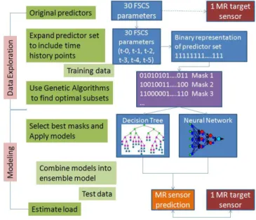
In this work, the experimental methodology consists of the application of computational intelligence and machine learning techniques in two phases: I) data exploration: characterization of the internal structure of the data and assessment of the information content of the predictor variables and its relation to the predicted (dependent) variables; II) modeling: build models relating the dependent and the predictor variables (Fig. 1). For phase (I) the Gamma test was used for estimating
Fig. 1. Experimental methodology.
the embedded dimension of the target series and was used in combination with genetic algorithms to find subsets of the predictor variables with modeling potential (i.e. input variables for function approximation techniques). These results were used as a base for model search at a subsequent stage. In phase (II) two different modeling techniques were used: Neural Networks (NN), and Model Trees (MT) (Section III-C). NN are regarded as a black box technique, while MT are considered a white box one.
A. Data preprocessing
In order to overcome the effect of the different units of measurement of the input variables, which creates semantic incompatibilities, a normalization procedure for all variables was required. Among the different normalization approaches the one applied here transforms the mean of each variable to zero and its standard deviation to 1 (z-scores). With zero mean and unit variance, all variables have an equal chance to contribute to an output prediction and also have an equal weight on similarity and distance measures, which play a crucial role in the nonlinear space transformations and the gamma test techniques.
From the point of view of the relationship between the predictors and the target in Eq.7, there are 2180− 1
combi-nations. They were explored using genetic algorithms (single and multi-objective) aimed at minimizingVr (Eq. 5) as well
as the Gradient G and the proportion of predictor variables P Vr simultaneously (with P Vr defined as the ratio between
the cardinality of the subset of predictor variables considered and the total number of available predictors (180)). The rep-resentation chosen was based on binary chromosomes coding the characteristic functions of each predictor variable, so that the position of the 1 bits indicate whether the corresponding variable from the set of 180 predictors is chosen for assem-bling a multivariate vector used as input variables for theVr
computation. In particular, the number of nearest neighbors for the computation of the two objectives related to the Gamma test was set to 25 after studying its variation over a broad range of neighborhood values (up to100). In order to explore the structure of the time dependencies within the FSCS and the MRNBX variables, phase space methods [12] were used. In the case of the MRNBX series (denoted asT ), 30 time lags were considered (which cover its embedding dimension).
{T (t − 30), T (t − 29), · · · , T (t − 1), T (t)} (6) For the FSCS variables, a more complex setting was con-structed in order to capture the nature of the lagged interactions between the whole set of predictors. IfPk(t), denotes the k-th
FSCS time series (k ∈ [1, 30]), tuples describing the state of the systems in terms of the predictors and the target can be formed as
{[P1(t − τ ), · · · , P1(t)], [P2(t − τ ), · · · , P2(t)], (7)
· · · , [P30(t − τ ), · · · , P30(t)]}, T (t)
where τ is a maximum embedding lag for MRNBX and the curly brackets separate the predictor from the target components of the tuple. In this studyτ = 5 in order to cover a time span of approximately two times the embedding of MRNBX (they are sampled with a 1:8 frequency ratio). The tuples in Eq.6 determine a 30-D phase space, while those of the predictor part of Eq.7, a 180-D space.
Typically the data is divided into training and testing sets in a proportion that favors the training set. In the present case it could not be done. The data set contains 21426 181-D tuples and even with a50% training set the genetic exploration using gamma test related variables as objectives (Vr,G) would
become unpractical due to the high computing times involved. In order to compose a training set with manageable size while still containing a statistically representative sample of the whole dataset, k-means clustering was applied. Accordingly, 1000 clusters were formed using k-means with Euclidean distance and for each cluster, the data vector closest to its centroid was selected (the so called k-leader). This sampling procedure ensures that every pattern in the original data is represented in the training sample and at the same time that it is a reasonable large one for training purposes. Thus due to the above mentioned constraints, the training set was composed of 1000 vectors and the testing set of the remaining 20426.
For the single-objective GA experiments (SOGA) (Sec-tion III-B1) a binary string representa(Sec-tion was used with classi-cal one-point crossover and bit flip mutation. An additional pa-rameter was introduced for generating initial populations with different proportions between ‘0’ and ‘1’ bits. The purpose was to put different levels of pressure (bias) on evolving population spawning a broad range of abundance of predictor variables. In cases where that probability is small, subsets with a few predictors are favored and conversely when the probability is high. Table II shows the set of SOGA parameters, defining a collection of 450 GA experiments. In this case the objective was to minimizeVr (Eq. 5).
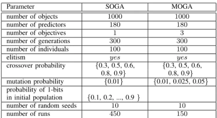
TABLE II
EXPERIMENTAL SETTINGS FOR THESOGAANDMOGA.
Parameter SOGA MOGA
number of objects 1000 1000 number of predictors 180 180 number of objectives 1 3 number of generations 300 300 number of individuals 100 100
elitism yes yes
crossover probability {0.3, 0.5, 0.6, {0.3, 0.5, 0.6, 0.8, 0.9} 0.8, 0.9} mutation probability {0.01} {0.01, 0.025, 0.05} probability of 1-bits
in initial population {0.1, 0.2, ..., 0.9 }
number of random seeds 10 10 number of runs 450 150
Considering that an ideal model would be one approximat-ing the target variable values as much as possible while beapproximat-ing simple and depending on as few predictor variables as possi-ble, a multi-objective optimization approach was investigated. For this purpose, a 3-objective problem was formulated aimed at finding subsets of predictor variables that simultaneously
i) minimize Vr as an approximation to the MSE of the
model’s residual, ii) minimize Γ (Eq. 4) as a measure of model complexity and iii) the ratio of the number of predictor variables in the model with respect to the total number of potential predictors (180). Table II shows the set of MOGA parameters, defining a collection of 150 GA experiments.
B. Modeling Techniques
Neural networks trained with the BFGS algorithm (Sec-tion III-C1) were obtained for the training set using two hidden layers and one output layer with (15-5-1) and (20-5-1) neurons respectively. Training was stopped when the mean squared error achieved the value of Γ in Eq. 4 in order to avoid overfitting. In the case of M5 models the training procedure used the parameters described at the end of (Section III-C2).
V. RESULTS
A. Data exploration results
Using the experimental settings shown in Table II, 450 runs of a single-objective GA aimed at minimizing Vr were
performed. The best two individuals had similar Vr values
(0.2662 and 0.2682 respectively) but different number of predictor variables (41 and 94 respectively). The small size of the first mask was not typical of the top 25 SOGA solutions, where the average subset size was 85 predictors.
In the second approach for searching subsets of input variables with predictor potential, an exploration using multi-objective GA with the NSGA-II algorithm was made with the experimental settings from Table II (150 runs). In this case the goal was to minimize simultaneously Vr, G and
P Vr. As is typical in real-world multi-objective optimization
problems, no single solution can absolutely optimize all of the objectives. The algorithm produces a set of candidate solutions representing the best tradeoffs between the different objectives (the non-dominated solutions). Each individual MO
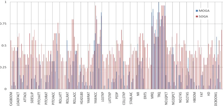
Fig. 3. Frequency distribution of predictor variables (6 time history points each) in the best 25 solutions obtained with single and multi-objective GAs.
Fig. 2. Objective spaces for the two best compromise solutions obtained with multi-objective GA . Note the typical upward curvature to the approximation of the Pareto front given by the set of (NSGA-II) non-dominated GA-solutions. The two selected runs (93 and 36) were the individual solutions with the closest distance to the origin. Left: run 93. Right: run 36.
solution is a vector in the objective space and the criterion used for ranking them was their module. It represents the Euclidean distance to the origin, which would represent a solution with no residual variance (Vr= 0. That is, a perfect
fit model), a perfectly smooth model (G = 0) and no predictor variables (clearly a physical impossibility, but just indicating a minimum of predictors requirement). Using such a criterion, the two ‘best’ solutions were chosen for model building using the training set. For them Vr = 0.1049, G = 0.0342,
P Vr= 0.1889 (34 predictors) and Vr= 0.1175, G = 0.0409,
P Vr = 0.1833 (33 predictors) respectively. These subsets
therefore contain less than 20% of the total available predictor variables (180). They belong to MOGA runs 93 and 36, whose final feasible solutions in the objective space are shown in Fig. 2. They both show the approximation to the Pareto fronts as concave-upwards surfaces bent as the coordinate origin is
approached, as expected for a three-objectives minimization problem.
The chart in Fig. 3 shows the frequencies of the predictors for the 25 best masks obtained through the single-objective and multi-objective GAs. The distribution of the frequencies across the predictors reflects the difference in the average size of the masks found by the two methods. These results provide some insight into the predictor/target relationship between the FSCS parameters and MRNBX for the flight condition examined in this work, forward level flight at full speed. The SOGA results show that none of the FSCS parameters were consis-tently eliminated from the subsets, while a number of FSCS parameters were consistently eliminated from or appeared with low frequency in the MOGA subsets (roll attitude, longitudinal and latitudinal stick position, stabilator position, retreating tip speed, temperature, and altitude). Three FSCS parameters were consistently identified as very important inputs as almost all of their 6 time history points were included: yaw acceleration, main rotor speed, and tail rotor speed. The relevance of the time history points as seen in the chart illustrate the importance of the time dependencies of the predictor variables in estimating the target sensor.
B. Modeling results
The best two masks found by the SOGA were used to build models using the training set, which comprises two neural networks trained with the BFGS algorithm, a model tree and an ensemble model averaging these. The results obtained on the testing set are shown in Table III (where rmse= root mean squared error, corr= correlation coefficient).
The results of the neural networks and the model trees were of the same order in terms of both rmse and correlation,
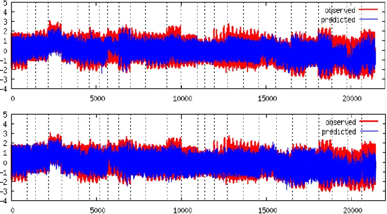
Fig. 4. Main rotor blade normal bending prediction based on ensemble models. Horizontal axis is sample number. Vertical axis is normalized MRNBX. Top: Ensemble model prediction using the best two subsets found by single-objective GA minimizing Vr. Bottom: Ensemble model prediction using the best two
subsets found by the MOGA NSGA-II algorithm (44 predictors) minimizing 3-objectives. Models were built using BFGS neural networks and M5 model tree techniques. For illustration purposes, the 27 distinct flight records were juxtaposed, each representing an individual time series separated by vertical dashed lines.
TABLE III
SINGLE-OBJECTIVEGATESTING SET RESULTS.
BFGS Neural Networks architecture 15-5-1 20-5-1 15-5-1 20-5-1 mask 1 1 2 2 Ensemble rmse 0.7591 0.7498 0.6519 0.6445 0.6189 corr 0.6953 0.6958 0.7690 0.7713 0.7875 M5 Model Trees mask 1 2 Ensemble rmse 0.7806 0.7010 0.6737 corr 0.6423 0.7234 0.7395
BFGS Neural Networks and M5 Model Trees
model Ensemble
rmse 0.6104
corr 0.7923
although slightly better for the neural networks. The models built from the second mask (with 94 predictors) yielded slightly better results than for the first mask using either M5 model trees or BFGS neural networks. It is interesting to note that while the first mask comprised less than half as many predictors as the second mask (41 vs 94), the omission of these predictors had little effect on the model results. The overall best is obtained with the ensemble of all individual models (rmse=0.6104 and corr=0.7923) indicating not only a reasonably good approximation of the MRNBX values, but also a good phase follow up of the signal, even though the
entire dataset is composed of records obtained at different times. The behavior of the ensemble model on the testing set is shown in Fig. 4(Top), from which it can be seen that although the model has a general good behavior, it consistently under-predicts the target signal, thus providing lower bound (i.e. conservative) estimates.
TABLE IV
MULTI-OBJECTIVEGA (NSGA-II)TESTING SET RESULTS.
BFGS Neural Networks architecture 15-5-1 20-5-1 15-5-1 20-5-1 mask 1 1 2 2 Ensemble rmse 0.7584 0.7377 0.7846 0.7974 0.6186 corr 0.7096 0.7343 0.6975 0.7067 0.7938 M5 Model Trees mask 1 2 Ensemble rmse 0.7534 0.7851 0.7146 corr 0.7016 0.6474 0.6964
BFGS Neural Networks and M5 Model Trees
model Ensemble
rmse 0.5928
corr 0.8006
The performance of the models obtained using the best two MOGA subsets on the testing set is shown in Table IV. The results obtained by the neural networks and the model trees are similar (although slightly better for the model trees). The behavior of the MOGA ensemble model on the testing set is
shown in Fig. 4(Bottom). Overall, the MOGA results are better than those for SOGA in terms of both rmse and correlation, but by a small margin. However, it is interesting to observe that the MOGA (NSGA-II) algorithm found subsets with i) significantly smaller number of predictor variables and ii) smallerVrvalues. This effect can be appreciated when looking
at the the model trees for the single and multi-objective cases: the former has 5 rules (in two model trees) with large linear regression terms, while the latter has only 3 rules in the two model trees with much smaller number of variables in the linear regression expressions.
The plots in Fig. 4 show how well the models were able to predict the main rotor blade normal bending as compared to the observed data. The upper and lower plots are almost undistinguishable; however, in certain sections, such as the first 3 flight records and those between samples 15000-18000, the superior performance of the MOGA models is noticeable. Overall, the models provide a fairly good prediction for the target parameter. Certainly the upper peaks are underestimated, the lower peaks less so, and overestimation of the values is rare. The main and secondary peaks as well as the phase of the predicted signal match up well with the target signal, which are important features for helicopter load monitoring.
It is important to keep in mind that the test data were taken from 27 different flight records with different aircraft configurations whose variation was not necessarily captured in the 30 FSCS parameters. Furthermore the training set was smaller than the test data set in a ratio of 1:21. Perhaps increasing the size of the training set, for example from 1000 to 2000 points, would improve the performance of the models without demanding overly high computing times. Even so, the results presented here are promising especially given the relatively small size of the training data set and that the predictor set to obtain these results, in the case of the MOGA models, used less than 20% of the total predictor variables.
The highlights of the approach used in this work, not typically found in traditional methods, include: i) assessment of predictive potential of variables and internal structure of data, ii) inclusion of time dependencies of variables, iii) use of white box techniques (MT) in addition to black box ones (NN), and iv) accounting for large variation in the flight condition in the training data. The inclusion of these aspects makes for a more robust, statistically sound approach to the problem of helicopter loads estimation.
VI. CONCLUSIONS
This work studied the use of evolutionary computation methods to assist in estimating helicopter dynamic loads. Us-ing sUs-ingle and multi-objective genetic algorithms to optimize residual variance, gradient, and number of predictor variables, subsets of the input variables were found that generated reasonably accurate and correlated models of the main rotor blade normal bending during forward level flight at full speed. From the set of 30 flight state and control system parameters and their time histories used as input variables, a large amount of irrelevant and/or noisy information was discovered and
identified, reducing the predictor set to less than 20% of the original size using multi-objective genetic algorithms. The frequency distribution of the predictor variables for the best GA subsets provides some insight into the possible physical process behind the input/output parameter relationship for this flight condition. The next task will be to extend the scope and complexity of the output parameters and flight conditions and work towards the goal of accurately estimating the dynamic loads on the helicopter indirectly for its entire usage spectrum.
REFERENCES
[1] T. B¨ack, D. Fogel, and Z. Michalewicz. Handbook of Evolutionary
Computation. Institute of Physics Publishing and Oxford Univ. Press, UK, 1997.
[2] E.K. Burke and G. Kendall. Search Methodologies: Introductory Tutorials in Optimization and Decision Support Techniques. Springer Science and Business Media, New York, 2005.
[3] K. Deb, A. Pratap, S. Agarwal, and T. Meyarivan. A fast and elitist multi-objective genetic algorithm - NSGA-II. Technical Report 2000001, Kanpur Genetic Algorithms Laboratory, 2000.
[4] K. Deb, A. Pratap, S. Agarwal, and T. Meyarivan. A fast and elitist multiobjective genetic algorithm: NSGA-II. IEEE Trans. on Evol. Comput., 6 (2):182–197, 2002.
[5] D. Evans and A.J. Jones. A proof of the gamma test. Proc. Roy. Soc.
Lond. A, 458:1–41, 2002.
[6] D. Goldberg. Genetic Algorithms in Search, Optimization, and Machine
Learning. Addison-Wesley Professional, 1989.
[7] J. G´omez-Escalonilla, J. Garc´ıa, M.M. Andr´es, and J.I. Armijo. Strain predictions using artificial neural networks for a full-scale fatigue monitoring system. In Proc. 6th DSTO Int. Conf. on Health & Usage
Monitoring, Melbourne, Australia, March 2009.
[8] D.J. Haas, J. Milano, and L. Flitter. Prediction of helicopter component loads using neural networks. J. American Helicopter Society, 40(1):72– 82, 1995.
[9] G. Holmes, M. Hall, and E. Frank. Generating rule sets from model trees. In 12th Australian Joint Conf. on Artificial Intelligence, pages 1–12, 1999.
[10] Georgia Tech Research Institute. Joint USAF-ADF S-70A-9 flight test program, summary report. Technical Report A-6186, Georgia Tech Research Institute, 2001.
[11] A.J. Jones, D. Evans, S. Margetts, and P. Durrant. The gamma test.
Heuristic and Optimization for Knowledge Discovery, 2002.
[12] H. Kantz and T. Schreiber. Nonlinear Time Series Analysis (2nd ed). Cambridge University Press, UK, 2003.
[13] A. Liu, C. Cheung, and M. Martinez. Use of artificial neural networks for helicopter load monitoring. In Proc. 7th DSTO Int. Conf. on Health
& Usage Monitoring, Melbourne, Australia, March 2011.
[14] J. Nocedal. Updating quasi-newton matrices with limited storage.
Mathematics of Computation, 35:773–782, 1980.
[15] F. Polanco. Estimation of structural component loads in helicopters: a review of current methodologies. Technical Report DSTO-TN-0239, Defence Science and Technology Organisation, 1999.
[16] J.R. Quinlan. Induction of decision trees. Machine learning, 1:181–186, 1986.
[17] J.R. Quinlan. Learning with continuous classes. In 5th Australian Joint
Conf. on Artificial Intelligence, pages 343–348, Singapore, 1992. [18] J.R. Quinlan. C4.5: programs for machine learning. Morgan Kaufmann,
San Francisco, CA, 1993.
[19] S. Reed and D. Cole. Development of a parametric aircraft fatigue monitoring system using artificial neural networks. In Proc. 22nd Symp.
Int. Committee on Aeronautical Fatigue, Lucerne, Switzerland, March 2003.
[20] R.Fletcher. Practical Methods of Optimization. John Wiley & Sons, 1987.
[21] A. Stef´ansson, N. Kon˘car, and A.J. Jones. A note on the gamma test.
Neural Computing and Applications, 5:131–133, 1997.
[22] Y. Wang and I.H. Witten. Induction of model trees for predicting continuous classes. In Proc. European Conf. on Machine Learning, pages 128–137, Prague, 1997.
[23] I.H. Witten and E. Frank. Data Mining: Practical Machine Learning