Assessment of a sulfur dioxide based diagnostic system in characterizing real time oil consumption in a diesel engine

Assessment of a Sulfur Dioxide Based Diagnostic System in Characterizing Real

Time Oil Consumption in a Diesel Engine

by

Mark A. Jackson

B.S., Marine Engineering; United States Coast Guard Academy, 1989

Submitted to the Department of Ocean Engineering and Mechanical Engineering in

Partial Fulfillment of the Requirements for the Degrees of

MASTER OF SCIENCE IN NAVAL ARCHITECTURE AND MARINE

ENGINEERING

and

MASTER OF SCIENCE IN MECHANICAL ENGINEERING

at the

Massachusetts Institute of Technology; May 1996

© 1996 Mark A. Jackson. All rights reserved.

The author hereby grants to MIT permission to reproduce and to distribute publicly, paper

and electronic copies of this document in whole or in part.

Signature of Author

._

-"Department of Ocean Engineering May 1996

Certified by_

...

Dr. Alan J. Brown

Professor, Department of Ocean Engineering

Thesis Advisor

Certified by

Dr. Victor W. Wong

Lecture Department of Mechanical Engineering

Thesis Advisor

Accepted by

.. _.--.,,

.

le

A. Douglas Carmichael, Chairman

Denartment Committee on Graduate Studies

Department of Ocean Engineering

Accepted by

A. Sonin, Chairman

Departmental Committee on Graduate Studies

Department of Mechanical Engineering

JASiSAI.Q--UETTS .NS'!i' rE OF TECHNOLOGY

Assessment of a Sulfur Dioxide based diagnostic system in

characterizing Real-Time Oil Consumption in a Diesel Engine

by Mark A. Jackson

Submitted to the Department of Ocean Engineering and the Department of Mechanical Engineering in Partial Fulfillment of the Requirements for the Degrees of Master of Science in Naval Architecture and Marine Engineering and Master of Science in Mechanical Engineering.

ABSTRACT

A study of oil consumption characteristics was completed using a single cylinder direct injection diesel engine. The objectives included assessing the performance and procedures of a real time sulfur dioxide oil consumption system and studying oil consumption including testing the repeatability and variability through load changes, speed changes, air intake manifold pressure changes, and the performance of various ring packs.

The testing included six matrices. Three of the matrices conducted measured the steady state speed and load effects on oil consumption for three different ring pack configurations (Standard Ring Pack, reduced Oil Control Ring Tension, and Inverted Scraper Ring). A matrix was conducted to measure the effects of reduced intake manifold pressure with standard ring pack configuration. Two matrices were conducted to monitor speed and load transients. The transient testing included alterations of speed at two loads and the alteration of load at two speeds.

The first steady state matrix with the standard ring pack showed that the SO2based diagnostic

system is a viable means to measure oil consumption and is capable of delivering repeatable results. The second steady state matrix with the reduced oil control ring tension showed an increase in oil consumption by, on average, 10.5 times. The third steady state matrix with the inversion of the scraper ring showed an increase in oil consumption by, on average, 6.4 times. The reduction of the intake manifold pressure to 90 kPa and 80 kPa caused increases in oil consumption by 84.2% and 165.5% respectively. This increase in oil consumption is likely caused by the differential pressure between the cylinder and the lands during the intake stroke. The two transient matrices showed that for small speed and load transients oil consumption measured by the SO₂diagnostic showed oil consumption "hump" in the positive and negative directions depending on speed or load.

Thesis Advisor: Alan J. Brown

Title: Professor, Department of Ocean Engineering Thesis Advisor: Victor W. Wong

ACKNOWLEDGEMENTS

I would like to thank the faculty at MIT Sloan Automotive Lab and that of the rest

of the Mechanical Engineering and Ocean Engineering Departments. You have made my

stay here at MIT challenging and rewarding. I would particularly like to thank Capt. Alan Brown and Dr. Victor Wong who have helped guide me through this thesis. Also, thanks to Prof. John Heywood for timely advise and overall perspective.

I cannot with any degree of consciousness mention anyone else before thanking

Tom Miller. Although we've known each other for many years I don't think either of us

had a clue how well we would truly end up knowing each other. Thank you for listening to my endless banter, and for helping when the "legacy" was about to break us. I really, couldn't have done it without you.

Richard Flaherty at Cummins Engine Company who answered my thousands of

questions and gave technical advice in solving some of my problems. Special thanks to;

Dave Fiedler of Dana Perfect Circle, Norbert Abraham and Weibo Weng also of

Cummins Engine Company.

I must thank my wife Suzanne who endured endless nights of me being the "ultimate of crabdom". You stood by me and were always very understanding. I

appreciate that more than you could know. Thanks.

I'd like to thank all those fellow students I worked alongside with at the Sloan Lab. To Tian Tian and Bouke Noordzij thanks for helping with those moments when my theories started to diverge. To Mark Kiesel thanks for asking all those questions that

made me delve deeper into the understanding of the system. To Alan Shihadeh thanks for

your patience with the engine. You put your work on hold and I deeply appreciate it. To

Brian Corkum, thanks for your assistance in, well, just about everything. I'd also like to

thank all the rest of the sloan students and staff who helped make life more pleasant and

enjoyable.

I'd also like to thank all of the Coast Guard and Navy students and staff who

made life more interesting, especially during those five class semesters. Lee, Tom Moore,

Chris Trost, Chris Warren, John D., Jim T., Dan P., Joc, Tim, Rob, Mike and Bob.

This project was primarily sponsored by the Maritime Administration (MARAD)

with support from the United States Coast Guard under contract DTMA 91-95-00051. Special thanks to Dan Leubecker of MARAD and Dr. Alan Bentz of the USCG R&D

Center for their guidance and support. This project was also supported by the Consortium

of Lubrication in Internal Combustion Engines, whose members include Dana

TABLE OF CONTENTS

ABSTRACT 3 ACKNOWLEDGEMENTS 5

TABLE OF CONTENTS

7

LIST OF FIGURES

9

LIST OF TABLES

11

ABBREVIATIONS 13 Chapter 1 MOTIVATION 15 1.1 Introduction 15 1.2 Previous Work 16

1.3 Oil Consumption Sources 16

1.4 Oil Consumption Measurement Techniques 17

1.5 Objectives 18

Chapter 2 EXPERIMENTAL APPARATUS

19

2.1 Engine 19

2.2 SO2 Diagnostic 22

Chapter 3 TESTING PROCEDURE

29

3.1 General Overview of Testing Procedure 29 3.2 Testing Procedure for the Standard Ring Pack 33

3.21 Test Matrix 1 33

3.22 Procedure

34

3.23 Matrix 1 - Engine Specifics, Controls and Variables 37

3.3 Testing Procedure Matrix a - Altered intake pressure

39

3.31 TestMatrix la

39

3.32 Procedure

39

3.33 Matrix la- Engine Specifics, Controls and Variables

39

3.4 Testing Procedure Matrix 2

3.41 Test Matrix 2 3.42 Procedure

3.43 Matrix 2 - Engine Specifics, Conti 3.5 Testing Procedure Matrix 3

3.51 Test Matrix 3

3.52 Procedure

3.53 Matrix 3 - Engine Specifics, Conti 3.6 Testing Procedure Matrix R

3.61 Test Matrix R 3.62 Procedure

3.7 Testing Procedure Matrix L 3.71 Test Matrix L 3.72 Procedure

Chapter 4 TEST CALCULATIONS

4.1 Determination of Engine Oil Consumption

40

40

40

rols and Variables 41

42

42

42

rols and Variables 43 43

44

44

45

45

45

47

47

I

Chapter 5 RESULTS AND ANALYSIS 53

5.1 Results of SO2 Uncertainty Analysis 53

5.11 Effect of Bypass Flow Rate

53

5.12 Effect of Various Sample Line Temperatures

56

5.13 Electronic Drift of Detector Output

57

5.14 Partially Completed Tests

59

5.2- Results for the Standard Ring Pack (Matrix 1)_ 61 5.21 Matrix 1: Steady State Speed and Load Effects on Oil 61

Consumption

5.22 Variability of Matrix I During Steady State Operation 62 5.3 Results for Various Intake Pressures (Matrix I a) 63 5.31 Results for Matrix la: Steady State Oil Consumption at 63

Various Intake Pressures

5.32 Results from Gas Flow and Ring-Dynamics Simulation 64 5.4 Results for Reduced Oil Control Ring Tension (Matrix 2) 65

5.41 Results for Matrix 2 65

5.42 Variability of Matrix 2 During Steady State Operation 66 5.5 Results for Inverted Scraper Ring (Matrix 3) 67

5.6 Results for Matrix R 68

5.7 Results for Matrix L 74

Chapter 6 CONCLUSIONS 81

Chapter 7 RECOMMENDATIONS

85

REFERENCES 91

Appendix A TESTING DATA SHEETS

93

Appendix B UNCERTAINTY ANALYSIS RESULTS

97

Appendix C MATRIX 1 RESULTS 103

Appendix D MATRIX a RESULTS 117

Appendix E MATRIX 2 RESULTS 128

Appendix F MATRIX 3 RESULTS

135

Appendix G MATRIX R RESULTS 144

LIST OF FIGURES

Figure 2-1 Figure 2-2 Figure 2-3 Figure 2-4 Figure 2-5 Figure 3-1 Figure 7-1 Figure A- 1 Figure A-2 Figure A-3

Figure A4

Figure B- 1 Figure B-2 Figure B-3

Figure B-4

Figure B-5 Figure B-6 Figure C- 1 Figure C-2 Figure C-3

Figure C-4

Figure C-5

Figure C-6

Figure C-7 Figure C-8 Figure C-9 Figure C- 10 Figure C- 11 Figure C- 12 Figure C-13

Figure C-14

Figure D-

Figure D-2

Figure D-3

Figure D-4

Figure D-5

Figure D-6

Figure D-7 Figure D-8

Figure D-9

Figure D- 10 Figure D-1 1

Intake System

Exhaust System

Oil Consumption Sampling System

Furnace Tube Setup

Bypass Flow Line Diagram

ISO 8178-4 Test Cycle Different Engine Applicati

Recommended Cell Air alteration

Overall Test Matrix

Daily Data Sheet

Oil Consumption Pre-Run Data Sheet

Oil Consumption Testing Data Sheet

Various Bypass Flow Rates

Sample Line Test (Line Temp @ 600°F)

Sample Line Test (Line Temp @ 950F)

Interval Test Series #1

Interval Test Series #2 Interval Test Series #3 Results: Test Matrix 1

Oil Consumption at Steady State (individual runs) Oil Consumption at Steady State (averages) Oil Consumption at Steady State (averages)

Oil Consumntion comparison with previous data

Oil Consumption at 1200 RPM and Low Load Oil Consumption at 1200 RPM and Med Load Oil Consumption at 1200 RPM and High Load Oil Consumption at 2400 RPM and Low Load Oil Consumption at 2400 RPM and Med Load... rosm o .t240RP.ad.. La

Oil Consumption at 2400 RPM and High Load Oil Consumption at 3200 RPM and Low Load Oil Consumption at 3200 RPM and Med Load Oil Consumption at 3200 RPM and High Load Results: Test Matrix 1 a

20

22

23

26

27

30

ions 86 93

94

95 96

97

98

99

100 101 102 103 104 105 106 107 108 109 110 111 112 113 114 115 116 117 OC at 1200 RPM and 5 Nm Various Press. (individual runs) 118 OC at 1200 RPM and S Nm Various Press. (averages) 119

OC at 1200 RPM and 5 Nm (90 kPa) 120

OC at 1200 RPM and 5 Nm (80 kPa) 121

Gas Flow at 1200 RPM and 5 Nm (101 kPa) 122 Gas Flow at 1200 RPM and 5 Nm (90 kPa) 123 Gas Flow at 1200 RPM and 5 Nm (80 kPa) 124

Mass Flow through Top Ring Gap

Intake Stroke

2nd

Land Pressures

Peak Pressures at Various Intake Pressures

125 126 127 -- -- -- - -- - - -J .... --

~~r-

J _ ... -- ... --- --- a- _ __ ___ .

LIST OF FIGURES (continued)

Figure E- 1

Figure E-2

Figure E-3

Figure E-4

Figure E-5

Figure E-6

Figure E-7

Figure F- 1

Figure F-2

Figure F-3

Figure F-4

Figure F-5

Figure F-6

Figure F-7 Figure F-8

Figure F-9

Figure G- 1 Figure G-2 Figure G-3

Figure G-4

Figure G-5

Figure G-6

Figure G-7 Figure G-8 Figure G-9

Figure G-10

Figure G- 11 Figure G- 12 Figure G- 13 Figure G- 14 Figure G- 15 Figure G- 16 Figure G-17 Figure H- 1 Figure H-2 Figure H-3 Figure H-4 Figure H-5 Figure H-6 Figure H-7

Results: Test Matrix 2 128

Oil Consumption at 52% OC Ring (individual runs)

129

Oil Consumption at 52% OC Ring (averages) 130 OC at 1200 RPM and 5 Nm with 52% OC Ring 131 OC at 1200 RPM and 10 Nm with 52% OC Ring 132 OC at 2400 RPM and 5 Nm with 52% OC Ring 133 SO2 at 2400 RPM and 10 Nm with 52% OC Ring 134

Results: Test Matrix 3 135

Oil Consumption with Inverted Scraper (individual runs) 136

Oil Consumption with Inverted Scraper (averages)

137

OC at 1200 RPM and 5 Nm with Inverted Scraper 138 OC at 1200 RPM and 10 Nm with Inverted Scraper 139 OC at 2400 RPM and 5 Nm with Inverted Scraper 140 OC at 2400 RPM and 10 Nm with Inverted Scraper 141

OC Comparison for various Ring Pack Designs

142

OC Comparison for various Ring Pack Designs

143

Speed Transient 2400-3200 at 5 Nm #1 144 Speed Transient 2400-3200 at 5 Nm #2 145 Speed Transient 2400-3200 at 5 Nm #3 146 Speed Transient 2400-3200 at 5 Nm #4 147 Speed Transient 2400-3200 at 10 Nm #1 148

Speed Transient 2400-3200

Speed Transient 2400-3200

Speed Transient 2400-3200

Speed Transient 3200-2400

Speed Transient 3200-2400

Speed Transient 3200-2400

Speed Transient 3200-2400

Speed Transient 3200-2400

Speed Transient 3200-2400

Speed Transient 3200-2400

Speed Transient 3200-2400

Speed Transient 3200-2400

Load Transient

Load Transient

Load Transient

Load Transient

Load Transient

Load Transient

Load Transient

(5-10 Nm)

(5-10 Nm)

(5-10 Nm)

(5-10 Nm)

(5-10 Nm)

(5-10 Nm)

(5-10 Nm)

at 10 Nm #2

at 10 Nm#3 at 10 Nm #4 at 5 Nm #1 at 5 Nm #2 at 5 Nm #3 at 5 Nm #4

at 10 Nm#l

at 10 Nm #2 at 10 Nm #3 at 10 Nm #4 at 10 Nm #5 at 2400

at 2400

at 2400 at 2400 at 3200 at 3200 at 3200 149 150 151 152 153 154 155 156 157 158 159 160 161 RPM #1

RPM #2

RPM #3

RPM #4

RPM #1 RPM #2 RPM #3 162 163 164 165 166 167 - __ - - -,

LIST OF FIGURES (continued)

Figure H-9

Figure H- 10

Figure H- 11

Figure H-12

Figure H-13

Figure H-14

Figure H- 1 S Figure H- 16 Figure H- 17

Load Transient (10-5

Load Transient (10-5

Load Transient (10-5

Load Transient (10-5

Load Transient (10-5

Load Transient (10-5

Load Transient (10-5

Load Transient (10-5

Load Transient (10-5

Nm) at 2400 RPM #1

Nm) at 2400 RPM #2

Nm) at 2400 RPM #3 Nm) at 2400 RPM #4 Nm) at 2400 RPM #5 Nm) at 3200 RPM #1 Nm) at 3200 RPM #2 Nm) at 3200 RPM #3 Nm) at 3200 RPM #4 169 170 171 172 173 174 175 176 177 - -__ --

-LIST OF TABLES

Table 3-1 Table 3-2 Table 3-3 Table 3-4 Table 3-5 Table 3-6 Table 3-7 Table 3-8 Table 3-9 Table 3-10 Table 3-11 Table 3-12 Table 3-13 Table 3-14 Table 3-13 Table 5-1 Table 5-2 Table 5-3 Table 5-4 Table 5-5 Table 5-6 Table 5-7 Table 5-8 Table 5-9

Table 5-10

Table 5-11 Table 5-12 Table 5-13 Table 5-14 Table 5-15 Table 5-16 Table 5-17 Table 5-18 Table 5-19 Table 5-20 Table 7-1

Differences in Test Matrices Test Matrix 1

Typical Run of Matrix

Diesel Fuel Characteristics

Ring Specifications

Matrix 1 Variable Specifics

Matrix la

Matrix 2

Typical Run of Matrix 2

Modified Oil Control Ring Speci

Matrix 3

Matrix R

Typical Run of Matrix R Matrix L

fications

Typical Run of Matrix L

Uncertainty Tests

Results Bypass Flow Test Results Sample Line Test Results Interval Test #1 Results Interval Test #2 Results Interval Test #3 Results Matrix 1 Results Matrix a Results Matrix 2 Results Matrix 3

Results Matrix R - Test R 1 BC 1 A

Results Matrix R - Test R1BC2A

Results Matrix R - Test RICB 1A

Results Test R I CB I A area of hui Results Matrix L - Test L 1B 12A Results Test L 1B 12A area of hun Results Matrix L - Test L 1 C 2A Results Matrix L - Test L1 B2 A Results Test L 1 B2 I1A area of hun

Results Matrix L - Test LIC21A

Recommended Variables to Mon"

31 33 36 37 38 38 39

40

41

42

42

44

45

45

46

53 54 57 58 58 59 61 63 65 67 69 71 72 73 76 76 77 78 79 79 88 -__ -- . S -- -4 - - - -- - -w _ A . , . L --

I-ABBREVIATIONS

DEFINITION

a AIRvolt b

BTDC

COmol CO2mol EXHtot FUELppm H2Oair H2Ocombmol H2Ocomb H2Oexh H2Owf Lubes MWexh OC Pa Pf Sexh SAIMPvolt

SOC

SPANppm SPANvolt T Va

# of carbon atoms per fuel molecule

Meter voltage output due to sulfur in ambient air

# of hydrogen atoms per fuel molecule

Before top-dead-center

Carbon monoxide concentration in exhaust

Carbon dioxide concentration in exhaust

Exhaust flow rate

Sulfur content in fuel

Water in ambient air

Water in exhaust due to combustion

Water in exhaust due to combustion

Water in exhaust

Fraction of water in air

Relative air to fuel ratio

Sulfur content in lubricating oil

Molecular weight of exhaust gases

Oil Consumption

Density of air

Density of fuel

Sulfur dioxide flow rate in exhaust

Detector output for OC reading

Specific oil consumption

Span gas ppm by weight

Output voltage from the detector due to span gas

Temperature

Volumetric air flow rate

volt

% molar

% molar

g/hr ppm by wt % by wt

% molar

% by wt

% by wt

% by wt

g/g-mole

gg/cyl-cycle

g/m3 g/cc

g/hr

volt

g/kW-hr

ppm by wt

volt

Celsius

m3f/hr

SYMBOL

UNITS

Vf

Volumetric fuel flow rate

cc/hr

y Relative hydrogen to carbon ratio

Chapter 1 MOTIVATION

1.1 Introduction

The United States has become very conscious of the ever growing pollution

problems existing throughout the country. Strict regulations have been implemented by

the EPA on heavy-duty diesel particulate emissions. The standard particulate rate for

1996 urban buses is 0.05 g/bhp-hr [20]. It also has become a concern in the marine

environment where emissions up to this point have not been regulated. In states such as

California cases have been noted of officials forcing ships to be towed out to sea 12 miles

before allowing the ship to start their engines. The Maritime Administration (MARAD)

has shown interest in knowing the relationship between lubricating oil consumption and

particulate emission rates. The amount of lube oil derived particulate of the overall

particulate rate was reported by Laurence [1] to be between 24-33% in a small light-duty

engine. With a significant portion of the particulate rate coming from the oil more

analysis is necessary to further the understanding of the relationship. In the past decade

new and improved methods have been introduced to study lubricating oil consumption in

engines. Most of the older methods have been "time-averaged". They required many

hours of study with results which had many errors. The sulfur dioxide tracer technique is

a "real-time" measurement system. It responds as the engine oil consumption changes.

Cummins Engine Company designed and built a real time oil consumption diagnostic

which utilized the SO

2

tracer technique. In the spring of 1995 Cummins loaned this

apparatus to M.I.T. for the purposes of research.

First uses of the system showed that oil consumption at specific speeds and loads

on various engines had unexplained variability. The newness of the system left some

uncertainty as to the cause of this variability. The SO2diagnostic, although an excellent

method to measure oil consumption, was untested as to its limitations and possible errors

introduced by the diagnostic itself.

In the past, attempts to take oil consumption and particulate data simultaneously

had been thwarted for various reasons. The relationship between the two is necessary to

fully understand what the effects of altering oil consumption has on particulate emissions.

1.2 Previous Work

In recent history many studies of oil consumption have been completed at M.I.T..

Most recent studies included the use of a tritium radio-tracer technique, by Lusted [3] and

by Hartman [4], and a sulfur dioxide tracer technique, by Schofield [9], to measure oil

consumption rates. All of these studies revealed large unexplained oil consumption

variability at particular speeds and loads. Lusted [3] studied the oil consumption behavior

in a production four cylinder spark ignition engine and found a variability of greater than

20% at one specific speed and load. Hartman [4] conducted similar oil consumption

measurements on a single cylinder Kubota diesel engine and his results showed a large

unexplained variability at one speed and load. Schofield [9] studied the oil consumption

behavior of a Ricardo Hydra single-cylinder direct injection naturally aspirated diesel

engine. Schofield used an SO2 diagnostic to measure the oil consumption and found a

similar variability at one specific speed and load. Thus far, no justification has been determined to describe this phenomena, but it has been hypothesized by Schofield that this large variability may be due to ring dynamics within the cylinder.

1.3 Oil Consumption Sources

Hill [6] describes four primary paths of oil consumption in diesel engines.

1.

Piston-ring-liner system

2. Overhead valve seals

3. Crankcase ventilation system

In this study, since the crankcase ventilation is not coupled with the air inlet and there is no turbocharger, the oil consumption can primarily be attributed to the piston-ring-liner system and the overhead valve seals. These two sources can be separated for oil consumption measurements utilizing a separate closed loop valve train oil system. If a "zero sulfur" oil is utilized in the valve train then any valve seal oil consumption would

be masked using the SO

2

technique. This study is focusing on overall oil consumption

and not on any particular sources. It is also coupled with a study on particulate emissions.

Since the source of the emission is irrelevant, the isolated valve train is not used.

1.4 Oil Consumption Measurement Techniques

Oil consumption measurement methods have varied greatly over the past 50 years.

There are two primary categories of measurement systems, time-averaged and real-time.

Up until the early '90's the most common method of measurement was time-averaged. In

those cases any transient behavior was hidden as was any true variability.

The most simplistic method to measure oil consumption consists of the "weight"

method. The weight method entails the weighing of the oil prior to running the engine

and then again after running the engine a known time period. This method requires a time

constant which is "very long" for any degree of accuracy. The longer the time run the better the results. This method has advantages in that it doesn't require any special

apparatus nor does it require additives or special fluids which might alter the operation of

the engine itself. Its disadvantages are that it requires such long periods of running to get

one data point and it is unknown what goes on in the engine during those times.

Another method is the tritium radio-tracer technique. The radio-tracer technique

requires a radioactive dye to be placed in the oil which is "traced" over a "long" time

period (approx. 10 min). This method decreases the time constant significantly but it still

lacks any real-time capability. Its advantages are that it doesn't require that the engine be run for days, but due to the difficulty in actually measuring the radioactive dye in the

exhaust it requires "long" time constants. It also has the disadvantage of requiring

radioactive material in the engine to run these tests. This requires special certification and

special caution in all aspects of testing.

A sulfur dioxide method was developed in the late 80's and early 90's. Its mode

of operation is to analyze the exhaust gas of an engine. A "zero sulfur" fuel and a relatively high sulfur oil are run in the engine. Sulfur dioxide found in the exhaust is

produced from the lubricating oil which is consumed. A system was prototyped by

Cummins Engine Company and loaned to MIT for use. This diagnostic was used

extensively by Schofield [9] in measuring steady state results.

1.5 Objectives

The large oil consumption variability found in many of the previous works was

hypothesized as being due to ring dynamics, the diagnostic equipment, or other

undetermined factors. This thesis work, sponsored by a joint Maritime Administration

(MARAD) and Coast Guard committee will focus on meeting the following objectives:

1. Providing oil consumption characteristics for different ring pack

configurations and air intake manifold pressures.

2. Assessing the SO2 diagnostic as a possible source of oil consumption

variability.

3. Eliminating or confirming ring dynamics as a contributor to oil consumption

variability.

A Ricardo Hydra single-cylinder direct injection naturally aspirated diesel engine

configured by G. Cussons Ltd. is used as the test bed for the study.

Chapter 2 EXPERIMENTAL APPARATUS

2.1 The Engine

The engine used in this experimental study was a Ricardo Hydra single-cylinder

direct injection naturally aspirated diesel engine configured by G. Cussons Ltd. It was

setup in a research test cell with separately mounted oil and water pumps. The engine

startup and load monitoring were accomplished utilizing a Dynamatic dynamometer and

variable speed coupling mounted on the engine drive shaft. Fuel flow, air flow, load and

engine speed were each controlled independently. Engine specifics are listed below.

Manufacturer: G. Cussons Ltd.

Model: Hydra single cylinder research engine

Bore: 80.26 mm Stroke: 88.9 mm Cylinders: 1 Swept Volume: 0.4498 1 Compression Ratio: 19.8:1

Aspiration:

Natural/Throttled

Rated Speed:

4500 RPM

Due to the limitations of the dynamometer, the maximum speed of the engine in

the current design is 3400 RPM. The manufacturer suggests that the engine's power be

limited by the exhaust smoke. The maximum power output is 8 kW at a smoke level of 4

Bosch units at 4500 RPM.

The engine's speed was set using the dynamometer controller. The controller is

capable of running at a set speed or a set load depending on the selected operating mode.

When the engine's speed was controlled the load was adjusted by altering the fuel flow.

The dynamometer uses resistive torque to control the speed which was set at the

operating condition, and ranged from 10-20% throughout the range of operation. In this

work, when load is referenced it refers to the average load. The load was monitored by a

load cell which was calibrated prior to the commencement of testing and monitored

thereafter. The load cell was attached directly to the controller and had an outlet which

allowed for monitoring via the data acquisition system.

The dynamometer controller was never set to the "load" operating mode during

testing. When in that mode the dynamometer controller maintains a constant load. This causes the engine to slow down or speed up depending on the fuel flow rate. It was too difficult to maintain a steady engine speed in this mode for any kind of steady state to be

reached.

The fuel flow was controlled remotely by a servo motor. The fuel flow was monitored using a "paddle wheel" flow meter. The flow meter was calibrated prior to use. The fuel injection timing was also controlled independently. The cylinder pressure was

monitored during operation via an oscilloscope to ensure timing was set to maximize

torque and engine performance.

The intake was equipped with a valve so that the air intake manifold pressure could be altered. A mass flow meter and a pressure transducer were placed in the intake line to monitor pressure and flow. Both instruments were calibrated prior to use. A diagram of the intake system can be seen in Figure 2-1.

Air Flow

ermocouple

Filter

Ex

Thermocouples were placed at several locations on the engine to monitor engine

operating condition. Thermocouple locations are listed below:

Thermocouple

Description

Number

1 VALVE OIL

2

FUEL IN

3 OIL INTO BLOCK

4 COOLANT TANK

5

EXHAUST MANIFOLD

6

AIR INTO HEAD

7

EXHAUST MIXING TANK

8 OIL OUT OF SUMP

9 INOPERATIVE

10 OIL INTO THE BLOCK

11

COOLANT TANK (ENGINE)

12 INOPERATIVE

13

COOLANT INTO ENGINE

14

CYLINDER COOLANT OUT

15

HEAD COOLANT OUT

16 INOPERATIVE

The exhaust system was modified to facilitate the taking of all data. A

1/4

in

stainless steel line was introduced right after the exhaust manifold to extract a sample for

the SO

2

diagnostic. A mixing tank is approximately one meter downstream from the

exhaust manifold. At the mixing tank fittings were added to allow for the monitoring of

the gaseous emissions content by two methods. The two methods were the ENERAC

2000 and the gas cart. A comparison was made of these by Miller [21 ]. After the mixing

tank the exhaust gas was funneled to the dilution tunnel for particulate sampling or the

exhaust trench for removal from the facility. The particulate sampling system is described

by Miller [21]. The valve (labeled # in Fig 2-2) which leads to the trench was used as a

back pressure valve. This will be described in more detail in the description of the SO

2

diagnostic.

To S02

System

Shop Air

ution

nnel

,Particulate

Filters

To Trench

Fig 2-2

The oil usedin the engine was a special 30W oil made by Lubrizol. This oil was

chosen for its specific performance characteristics. This oil, when compared to most

standard oils, has an even sulfur distribution throughout the distillation range of the oil.

This was also noted by Ariga [7]. The even sulfur distribution ensures that for any

operating condition (cylinder temperatures) an equivalent amount of sulfur is released.

This makes results more precise and comparable over various speeds and loads.

2.2 The SO2 Diagnostic

The oil consumption was measured using a pyrofluorescence sulfur dioxide

testing diagnostic developed by Cummins Engine Company, Inc. The principle of this

gas. This is made possible by using a "zero sulfur" oil and lubricating oil which contains

sulfur. The system is diagrammed in Fig 2-3.

The diagnostic was changed multiple times throughout testing. As one of the

objectives was to assess whether the diagnostic was the cause of the variable oil

consumption, changes were made in an attempt to improve the functionality of the

diagnostic. A brief description of the diagnostic in its initial state sets the foundation for

the alterations which were made.

Lch

- valve

Fig 2-3

Immediately following the exhaust manifold the exhaust gas is drawn through a

1/4

inch stainless steel tube (sample line). The sample line leads the gas through a solenoid

valve which allows for the isolation of the exhaust gases from the system during

calibration. Immediately following the solenoid valves is the furnace which is heated to

1000° C. The furnace is to ensure combustion of all particles in the exhaust gas. After the

furnace the gas flows through a 60gm filter which removes any remaining large particles,

which escaped combustion in the furnace, prior to entering the analyzer.

Heated lines maintain the temperature of the gas above the point of condensation.

Immediately prior to the analyzer a pair of membrane dryers remove the 3-12% water in

the exhaust directly from the vapor phase without condensing the moisture first.

The sample is then mixed with ozone to oxidize any NO to NO2. The sample is

then analyzed by a pulsed fluorescent ambient SO

2

detector. The detector's linear DC

voltage output is recorded by a computer data acquisition system and a linear chart

recorder.

The concentration readings were real-time measurements of the SO

2

concentration

and were proportional to the oil consumption of the engine. The details of the calculation of oil consumption from the voltages can be found in Chapter 4.

The real-time oil consumption (RTOC) system, being a prototype, was initially run at the original specifications. Those specifications are outlined by Schofield [9]. The initial focus in regard to the diagnostic was to determine whether any of the variability

associated with Schofield's data was due to the system itself. Through multiple

conversations with members of the Lube Oil consortium and Richard Flaherty of Cummins Engine Company it was theorized that part of the variability might be caused by the sample line being at too low of a temperature and too great a length (--42 in for Schofield's setup). In the literature generated about the system it was stated, "keep the sample line temperature above 600°F". The vaporization temperatures of typical oil range from 600-900°F (Flaherty[5]). It was decided to do two things; I1) Increase the

temperature of the sample line above the vaporization/condensing point of the oil (=950°F), and 2) To shorten the length of the sample line. As the length of the line increased the more oil was capable of becoming resident in the lines.

The sample line was installed with a length of 18 inches and temperatures were increased to greater than 950°F. The temperature increase included not only the sample line but also the line between the solenoid valves and the furnace. Another modification

which was along similar lines was the addition of insulation at the exhaust manifold. It

was insulated only to the sample line and no further. This was done in an attempt to

The system was operated in this configuration for approximately 15 test runs. At

that time it became a concern that the exhaust back pressure requirements might be

excessive. The system requires that pressure be applied to the exhaust system to get flow

to the analyzer. This was done by closing the back pressure valve on the exhaust (Valve #1 on Fig 2-2). The literature stated that 1.5 liters/min (/m) was required as a "bypass flow" to ensure that only exhaust gas was received at the SO2 detector and an accurate

reading was given. The bypass (see Fig 2-3) is a "vent" for the analyzer. The exhaust gas in the analyzer itself needs to be at atmospheric pressure. For this reason the bypass flow line was added to reduce or "vent" any excess pressure. The bypass line was periodically

monitored for flow using a "floating ball" flow meter installed with the system. Due to

this requirement of 1.5 1/m bypass flow a pressure transducer was installed in the exhaust system following the exhaust manifold, and prior to the sample line (see Fig 2-3) to monitor the back pressure on the engine. At the same time modifications to the sample line location were made. Initially the sample line was attached to the exhaust manifold perpendicular to the flow of the exhaust. It was chosen for ease of operation and it enabled us to have a "short" sample line. With the concern over back pressure it was

decided that the use of the engines flow would decrease the need to create pressure in the

exhaust line. The furnace and other apparatus were moved so that a more "direct" sample line could be installed. The sample line was placed such that the exhaust gas velocity was utilized in increasing flow (see Fig 2-4). No back pressure measurements were taken prior to the sample line change. For this reason it is unknown whether the new location

improved the flow and if so, to what degree.

While repositioning the furnace the glass furnace tube was broken. This tube was replaced several times during this operation and it became apparent that it was a weak

link in the system. The slightest misalignment caused a bending moment on the tube and

it would break. The engine's vibration during startup and shutdown also caused

breakage's to occur. A revised "bracing" system was designed and implemented. Previously, both ends of the tube were connected to stainless steel swagelock fittings.

These fittings were rigidly mounted to the furnace by steel braces. With alignment being a

problem it was decided that if the ends of the tube were mounted to flexible tubing the

tube would "float" in the furnace and would not be susceptible to misalignment or

vibration problems. It was decided to install this tubing only on the downstream end due

to a concern that oil and combustion particles might accumulate in the corrugations of the

flexible tubing prior to the furnace. This tube was installed as shown in Figure 2-4.

Furnace Tube Setup

Riou

COU]

Fig 2-4

After the new flexible tubing was installed the downstream end was capable of moving when necessary, but only minutely due to the packing material around the tube

itself as it exited the furnace. This arrangement worked satisfactorily with no more glass

tubes being broken.

The previous concern over maintaining at least 1.5 /m was erroneous. The

previous explanation was that the analyzer would utilize 1/m and the additional flow

(then thought to be 0.5 /m with a 1.5 /m bypass) was to ensure that only sample gas was reaching the analyzer. This additional flow is not 0.5 I/m, but actually all of the bypass flow is additional flow. A simplified line diagram can be seen in figure 2-5 which shows the flow. If the analyzer always draws 1 /m and the bypass is 1.5 l/m then the sample line

flow must be at least 2.5 /m assuming no losses. A sample line flow of only 1.5 1/m is

necessary.

Sample Line

Flow

_-

1 1/m

_{x,. %} 4. .g2f

Bypass Flow

Fig 2-5

It could be theorized that the excess bypass flow, an extra liter/min, would not

have any effect, but, it is possibly detrimental to the operation of the diagnostic. Any

reading at the bypass at all would ensure that the analyzer is getting a pure sample. The

excessive flow(1.5 Url/m) may have been detrimental in that it was causing the analyzer to become pressurized. The bypass flow was designed as a vent to ensure that the analyzer was at atmospheric pressure. Too much flow causes the bypass to be an inadequate vent. The uncertainty analysis (to be discussed in more detail in Chapter 5) showed that the change from 1.51/m to 0.5 U/m bypass flow altered the S02 concentration of a known span gas by 10%. There was also "unsteady" behavior at the higher bypass flow rates and none

at the lower flow rates. Overall, if the bypass is maintained at either level during

calibration and then during testing the results should be equivalent. However, the higher

flow rates required a much higher pressure be placed on the exhaust system. This could

be avoided by using the lower flow rates.

Following the installation of the flexible tubing and the new furnace tube it was noticed that the filters located after the furnace were clogging with soot more readily and

the furnace exit temperature was lower than before. The furnace tubes are filled with a

quartz substance. It was believed that the new furnace tube was not as tightly packed as the previously used tubes. For this reason the gas had less surface area to come in contact

within the tube and the temperature of the gas was not getting to the desired level. New

tubes were ordered. A change in design was made which increased the diameter of the

Analyzer

..ap __

-I

tube from 1 to 2 inches. This would increase the time the gas spent in the tube by four

times. With the new tubes in place the soot found in the filters was eliminated and the

exit temperature of the furnace was increased back to previous levels. No comparisons

were made of previous tubes and current tubes for exact change in exit temperatures or

soot accumulation. The system has been modified (i.e. distance to thermocouple, flexible

tubing, etc..) such that the study would prove inconclusive results.

At one point during testing it was detected that the signal coming from the analyzer was erratic. The analyzer itself was faulty and it was necessary to replace the lamp and the socket for the lamp. A check of the lamp voltage should be made

periodically to ensure proper functioning of the lamp.

The data acquisition system utilized was a 486/66 MHz computer with an Analog

to Digital card inserted. It was capable of monitoring a maximum of six channels

(normally eight, but two were found to be inoperative). The computer was set up to acquire real-time SO2 concentration, Engine Speed, Engine Torque (Load), Fuel Flow,

Air Flow, and CO

2

concentration of the exhaust gas. The signals were converted using

Global Lab software and then input into an Excel spreadsheet for conversion to oil

consumption.

The exhaust gases were monitored by two different sources, the MIT gas cart and

the ENERAC 2000. The gas cart was calibrated on a daily basis. The exhaust gases CO, CO2, NO and NOx were monitored manually. The ENERAC 2000 is a portable exhaust

gas measurement system. Its results were not used for any of the oil consumption

calculations. For a comparison between the ENERAC 2000 and the gas cart see Miller

[21].

Chapter 3 TESTING PROCEDURE

3.1 General Overview of the Testing Procedure

This chapter presents the testing procedure for the oil consumption data. The

actual testing was categorized into five matrices, 1, la, 2, 3, L and R. All of the matrices used zero sulfur diesel and Lubrizol 30W oil. Matrices 1-3 were generated in an attempt to match the typical duty cycle of a marine diesel engine operating near land (harbor). In order to determine what a "complete" marine diesel duty cycle would be, ISO 8178 Part 4

"Reciprocating Internal Combustion Engines- Exhaust Emission Measurement" was

evaluated. The test cycle for different engine applications as outlined in ISO 8178-4 are

shown in Figure 3-1.

Cycle Definitions are described as follows:

Cycle

Description

A Reference cycle for vehicle engines

B Universal cycle, applications similar to on -road service

C1

Off-road vehicles and industrial equipment, medium and high load

C2 Off-road vehicles and industrial equipment, low load

D

Constant speed applications, power plants

D2

Constant speed applications, generator sets with intermittent load

E1

Marine engine applications, pleasure craft engines

E2

Marine applications, constant-speed engines for ship propulsion

E3

Marine applications, heavy-duty propulsion engines

F

Locomotive applications

G1/G2

Small engines, utility lawn and garden

G3

Small engines, hand held equipment

ISO 8178-4 Test Cycle for Different Engine Applications

Idle

160

Percent of Rated Speed I Rated Speed

Cycle

Percent Load

0

10

25

50

75

100

10

25

50

75" '

100 A 0.25 0.08 0.08 0.08 0.08 0.25 0.02 0.02 0.02 0.02 0.10 B 0.25 0.08 0.08 0.08 0.08 0.25 0.02 0.02 0.02 0.02 0.10 C1 C2

Dl

D2

F

GI

I-'%

u

/-G3

El

E2

E3

I%Speed/%Load/Wt

63/25/0.15

180/50/0.15

91/75/0.5

]100/100/0.2

Fig 3-1

The duty cycles considered to be applicable for simulation of low speed marine diesel engine operations were cycle E2 (Marine Applications, constant speed engines for

ship propulsion) and cycle E3 (Marine Applications, heavy-duty propulsion engines).

Cycle E2 applies to constant speed diesel engines and is not applicable to this study. The unmodified version of the E3 duty cycle would require four engine test speeds and loads

-as shown in Figure 3-1. However, time constraints demanded that the scope of this study

be limited to ensure ample time for data analysis. Therefore, a modified version of the E3

cycle was selected to model operating conditions for low speed marine diesel engines.

The lowest recommended test speed for the E3 duty cycle, 63% of maximum, does not

adequately model near land or maneuvering operating conditions. For this reason, an

engine is a small bore, high speed diesel engine and the intent of this study is to model low speed marine diesel engines. For this reason, high end test speeds of 70% and 97% (2400 and 3200 RPM) vice 90%, 91% and 100% of maximum rated speed were

incorporated. These chosen values match the work done by Schofield [9] and Ford [10],

which is ideal for evaluating repeatability of test results, and they sufficiently cover the

suggested E3 duty cycle test speeds.

The modified E3 duty cycle utilized in this study includes three test loads vice two. -x mid-range test load was added to provide a more complete range of loading

conditions. This approach meets the requirements for this study and sufficiently

incorporates the guidance of ISO 8178 Part 4.

In addition to the modifications mentioned above, air intake manifold pressure

was varied for the low speed low load condition. This was to obtain a baseline indication of its effects. Two alternative ring pack configurations were chosen to include a reduced oil control ring tension and an inverted scraper ring. A summary of all six test matrices and their primary differences is given below in Table 3-1.

Table 3-1

Test Matrices , a, 2, and 3 were all conducted in conjunction with particulate

testing completed by Miller [21]. Tile transient tests for speed and load were done in

between steady state tests, but no particulate samples were taken. The engine was

overhauled twice to reconfigure the ring pack. Re-assembly of the engine was done such

Matrix

Ring Configuration

Intake Pressure

Test Condition

I

Standard

Atmospheric

Steady State

l a Standard 80 kPa, 90 kPa Steady State

2 50% OC Ring Tension Atmospheric Steady State 3 Inverted Scraper Ring Atmospheric Steady State

R

Standard

Atmospheric

Speed Transient

that the engine was as close to the original configuration as possible. No alterations were

made other than the rings with the exception of the hydrocarbon deposits which had

built-up on the cylinder liner. These deposits were removed each time to facilitate the removal

of the piston assembly.

A method to easily distinguish between all test runs and to label them appropriately was developed. Runs were labeled using the following coding system;

- Letter (A, B, C)

-

# (1-3)

-

Letter (A, B, C)

# (1-5)

For example; 2B IA3 - represents a run with a 50% oil control ring tension, at 2400 RPM with a 5 Nm load, at Standard atmospheric pressure, and it is the third run at this

operating condition. A similar system was put in place to monitor transient tests. It is as

follows;

Speed Transients;

R # (1-3) Ltr (A, B, C) Ltr (A, B, C) # (1-3) Ltr (A, B, C) # (1-5)

Type

Ring

Initial

Speed

Final Speed

Load

Intake Press.

Run #

Pack

Example; RlBC2A2 - Speed Transient, Standard Ring Pack, 2400 RPM * 3200 RPM,

10 Nm Load, Atmospheric Pressure, Run #2.

# (1-3)

Ring Pack

Speed

Load

Intake Pressure

Run #

I- Standard A - 1200 RPM I - 5 Nm A - Standard Press. I - Run #1 2-50% OC ring B - 2400 RPM 2 - 10 Nm B - 0 kPa 2 - Run #2 3-Invert Scraper C - 3200 RPM 3 - 15 Nm C -80 kPa

3

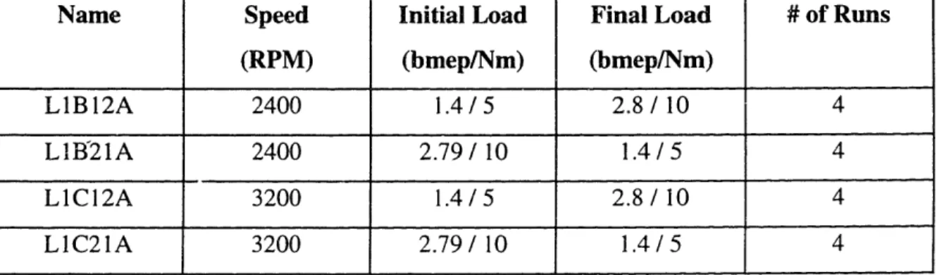
- Run #3

Load Transients;

Example; L1B21A4 - Load Transient, Standard Ring Pack, 2400 RPM, 10 Nm

zz

5 Nm

Load, Atmospheric Pressure, Run #4.

This system allowed for easy labeling and retrieval of computer files and general

organization.

3.2 Testing Procedure for the Standard Ring Pack

3.21 Test Matrix 1

Table 3-2 shows the details of Matrix 1.

Name Speed (RPM) Load (Nm/bmep) # of Tests

1A1A(1-4)

1200

LOW(5 Nm/1.4 bar)

4

1A2A(1-4) 1200 MED(10 Nm/2.8 bar) 4

1 A3A(1) 1200 HIGH(15 Nm/4.2 bar) 1

1B 1A(1-5) 2400 LOW(5 Nmrn/1.4 bar) 5

1B2A(1-4) 2400 MED(10 Nm/2.8 bar) 4

1B3A(1-2) 2400 HIGH(15 Nm/4.2 bar) 2

1C1A(1-4) 3200 LOW(5 Nm/1.4 bar) 4

1C2A(1-4) 3200 MED(10 Nm/2.8 bar) 4

1C3A(1-4)

3200

HIGH(15 Nm/4.2 bar)

4

Table 3-2

This matrix includes three speeds and three loads. Initially, four runs were planned for each condition. The high load condition was completed only once at low

speed and twice at medium speed due to the accumulation of particulates in the sample

line. With the back pressure remaining steady the bypass flow decreased by over 0.5

I/min over a period of 2-5 minutes. A decrease in bypass flow causes the calibration data

to be inaccurate for the test condition. An increase in back pressure would increase the

bypass but would alter the operating condition of the engine. This was decided to be a

problem to the system and not correctable at the time of testing. No further runs were

completed at high load. The medium speed-low load condition was previously noted to have variability by Schofield [9]. For this reason an additional run was conducted at that

speed and load.

3.22 Procedure

The engine was received and was immediately run for 50 hours to break in the oil. This was to ensure that the oil volatility and viscosity levels were at a steady state level and that the "high-end" sulfur compounds were released (Flaherty [5]).

Once the engine was broken in, testing commenced. Tests were run in random order to best ensure repeatability. A typical test day was started with the purging and

calibration of the SO2 diagnostic. This consists of purging the system with "Zero Air"

which is compressed air that all sulfur compounds have been filtered out. This occurs while the system is allowed to reach its operating temperature. While this is occurring the engine is warmed and prepared for operation. The gas cart, which consists of a Carbon Dioxide, Carbon Monoxide, Nitrogen Oxide, Nitrogen Dioxide, and Oxygen analyzers, was purged with Nitrogen and then calibrated. These were used to monitor gaseous

emissions for calculation of oil consumption and comparison with the ENERAC 2000

(see Miller [21]).

After zero air purging and warm up a known concentration of SO2 was introduced

to the system. This "span" gas was allowed to flow for a minimum of 6 minutes to allow for complete settling of the system. Once this was done the span pot on the front of the detector and/or the photomultiplier setting within the detector housing were set so the readout was identical to the concentration of the span gas. During this time, the linear

and a computer file respectively. An example of the data sheets is located in Figures A- 1 through A-3 in Appendix A.

The system was then again purged using zero air for a minimum of six minutes or

until the detector again settled on zero ( 0.005 ppm). While the system was being

calibrated the engine was being warmed at 3200 RPM and 4.2 bar bmep (15 Nm). This was done to ensure that the exhaust system and combustion chamber were heated to a point where any residual oil particles were vaporized in the system and the surrounding metal was heated such that no oil particles could condense.

Once the SO2 system was "zeroed" again the system was checked for 03

production. A 5000 ppm NO gas was introduced to the system and allowed to flow for approximately six minutes. Once the system was settled out, the 03 was secured. The

detector output was monitored for a "spike". Once the detector began spiking, the

03

was

re-energized. The detector was then allowed to zero again. The NO was disconnected. Span gas was again introduced to the system. This was to check the calibration and was again monitored by chart recorder and computer. The span gas was secured and the system was purged with zero air. Once the system was purged the exhaust gas solenoid valve was opened and the "gasses" valve was secured (see Fig 2-3). This allowed the engine exhaust gases to enter the system. With the exhaust gases valve open the exhaust back pressure valve was regulated to ensure proper bypass flow. In this case it was set at

1.5 /min. The system was allowed to settle out for approximately 45 minutes to an hour. Once the system settled at a test condition, data was taken.

For Matrices 1, l a, 2 and 3 testing consisted of runs of 40 minutes of data

acquisition. Once a run began, SO2concentration, RPM, Load, Fuel Flow, Air Flow, and

CO2 were monitored for the entire time. Miller took two particulate samples per run. The

particulate samples ranged from 5-20 minutes apiece (see Miller [21]). Manual

monitoring occurred of all other parameters of the engine and SO

2

diagnostic.

A typical time table was as shown in Table 3-3.

Time

Events

o0

min

-Computer Acquisition started monitoring

SO2,

RPM, Load, Fuel Flow, Air

Flow and CO2concentration.

- Manual recording started of C0

2

, CO, NO and NO,, via Gas Cart and

ENERAC 2000 (every 3 minutes)

5 min -Particulate Sample #1 commenced

10 min -Pre-Test operating parameters recorded manually 15-20 rin -Particulate Sample #1 completed

20 min -Engine operating parameters recorded

-Particulate Sample #2 commenced

30-35 min -Particulate Sample #2 completed

40 min

Test Ende

d

Table 3-3

At the completion of a days testing the engine solenoid valve was secured and the "gases" valve (see Fig 2-3) was opened. This allowed zero air to flow through the system and to allow a thorough purging of the diagnostic. Once the detector again reached zero, span gas was introduced to the system and the detector was again calibrated to check for drift in the detector. Any drift was taken into account with a linear interpolation of the morning and evening calibrations in the calculation for oil consumption.

The temperatures in the engine very often took up to an hour to reach steady state, especially the oil temperature. The temperatures had to be monitored carefully to

duplicate previous operating conditions. The oil consumption was calculated from data

collected in the first 10 minutes of testing. This required that the engine was at steady

state prior to commencing testing. The data was collected at a sampling frequency of 0.2

Hz or a point every five seconds. Once all data was collected at the 40 minute mark a new operating condition was set and the procedure was repeated for the entire matrix.

3.23 Matrix 1 - Engine Specifics, Controls and Variables

During the testing the engine was run with an ultra low sulfur diesel fuel so that it

would not contribute significantly to the overall sulfur dioxide concentration. Table 3-4

shows a summary of the diesel fuel characteristics.

API GRAVITY

39.8

FLASH POINT(°C)

68.9

POUR POINT(°C) -20.6 CLOUD POINT(°C) -23.3 VISCOSITY (Cs @ 40°C) 2.7 SULFUR(weight ppm) 0.1

HYDROGEN-CARBON RATIO

1.88

HEAT OF COMBUSTION (MJ/kg) 43.1

PARTICULATE MATTER (mg/l)

5.06

CETANE INDEX 55 CETANE NUMBER 42 Table 3-4

The lubricating oil was, as previously stated, Lubrizol 30W with a sulfur content of 1.27% by weight.

The ring pack configuration for test Matrix was the standard as set by

manufacturer's specifications. The first ring or compression ring was chrome plated and

slightly rounded in shape. The second ring or scraper ring was beveled. The third ring or

oil control ring was chrome plated with two rails and a separate coil spring for tension

control.

Table 3-5 shows the manufacturer's specifications.

Table 3-5 - Standard Ring-Pack Characteristics

The operating conditions for all runs were matched as closely as possible. During runs initial settings were made versus speed and load. Once these were set the exhaust temperatures and fuel flow rate were targeted. The following table shows the speed, target load, fuel flow rate, injection timing and exhaust temperatures.

Table 3-6 - Matrix 1 Variable Specifics

Ring Diameter (mm) Cold Gap (mm) Tension (N)

Compression 80.25 0.43 9.3

Scraper 80.25 0.43 8.2

Oil Control 80.25 0.51 53.8

Speed

Engine Load BMEP/Torque

Fuel Flow

Injection

Exhaust

(RPM)

(bar/Nm)

Rate

Ti.ning

Temperature

(cc/min) (°BTDC) (°C) 1200 LOW 1.4 / 5 8.0 9 240 1200 MED 2.8/ 10 10.9 9 321 1200 HIGH 4.2/ 15 14.0 9 395 2400 LOW 1.4 /5 16.4 14 300

2400

MED

2.8 / 10

22.0

14

365

2400 HIGH 4.2 / 15 29.0 14 475

3200

LOW

1.4 / 5

26.0

15.5

415

3200

MED

2.8 / 10

33.5

15.5

480

3200 HIGH 4.2 / 15 41.1 15.5 545

3.3 Testing Procedure Matrix la - Standard Ring Pack with altered Intake Pressure

3.31 Test Matrix la

Matrix 1 a utilized the same setup as Matrix with the single exception that the intake manifold pressures were altered. The matrix was setup as shown in Table 3-7.

Table 3-7

3.32 Procedure

The calibration of the SO

₂

diagnostic was completed as outlined in section 3.22.

The engine was adjusted to the 1200 RPM-5 Nm load and allowed to steady out. Once

steady, the throttle valve which was installed in the intake of the engine was slowly

closed while the intake pressure was monitored. When the intake pressure reached the

desired value the engine load was re-adjusted to the proper level, if necessary. The intake

was again monitored and adjusted as necessary. The throttle valve has only a "coarse" adjustment and a great deal of manipulation was necessary to reach the desired level. The

engine was then allowed to settle out. Engine parameters were monitored to ensure

steady state operation. These runs were intermixed with those of matrix 1 and the

procedure was identical to that which was outlined in section 3.22.

Name

Speed

Load

Intake Pressure

# of Tests

(bmep/Nm)

lAlB 1200 1.4 / 5 90 kPa 4

IAIC 1200 1.4 / 5 80 kPa 4

3.33 Matrix la Engine Specifics, Controls, and Variables

All of the engine specifics, controls, and variables were the same as in Matrix 1

with the exception of the air intake manifold pressure.

3.4 Testing Procedure for Matrix 2

3.41 Test Matrix 2

Table 3-8 shows the details of Matrix 2.

Name

Speed

Load

# of Tests

(RPM) (Nm/bmep)

2A I A(I -4) 1200 LOW(5 Nm/1l.4 bar) 4

2A2A(I1-4) 1200 MED(10 Nm/2.8 bar) 4

2B 1 A( 1-4) 2400 LOW(5 Nrn/ 1.4 bar) 4

2B2A(0) 2400 MED(10 Nm/2.8 bar) 0

Table 3-8

3.42 Procedure

The engine was dismantled following the completion of Matrix 1, a, R and L.

The head and piston assembly were removed. A new ring pack which had been modified

by Dana Perfect Circle was inserted. The same standard top and scraper ring which were used in previous testing were again used for the top two rings. The only difference was a lesser tension oil control ring. The tension was reduced to 28.0 N from an original tension of 53.8 N. This is a reduction to 52. 1% ring tension. The piston assembly and head were re-installed. The engine was checked and run to monitor for leaks.

before. The measurement of the oil consumption for these tests was above the range of the detector (> 2 ppm SO₂ concentration). The test procedure was modified slightly for

these tests. After calibration and system purging of the SO

2

detector the engine solenoid

valve was opened, but the gases solenoid was not closed. This allowed a flow of zero air

to flow into the system. The exhaust gases and zero air were mixed thus diluting the sample to the detector. The amount of zero air injected into the system was monitor:d

manually using the Tylan flow meters associated with the syste.n. A typical run's timeline

would appear as described in Table 3-9.

Time

Events

0

min -Computer Acquisition started monitoring SO2, RPM, Load, Fuel Flow, Air

Flow and CO

2

concentration.

- Manual recording started of CO2, CO, NO and NOx via Gas Cart and

ENERAC 2000, and zero air flow recorded.

5 min -Particulate Sample #1 commenced

10 min -Pre-Test operating parameters recorded manually -Zero air flow altered and recorded

15-20 min -Particulate Sample #1 completed 20 min -Engine operating parameters recorded

-Particulate Sample #2 commenced

-Zero air flow altered and recorded 30-35 min -Particulate Sample #2 completed

-Zero air flow altered and recorded

40 min

Test Ended _

Table 3-9

No data was recovered for test 2B2A. The dilution ratio became excessive and the

signal became erratic. (See Chapter 5)

Several levels of dilution were used in an attempt to better calibrate the dilution

ratios. With multiple concentrations and flow rates of dilution gases results were

accurately obtained.

3.43 Matrix 2 Engine Specifics, Controls, and Variables

All of the engine specifics, controls and variables were the same as Matrix 1 with

the exception of the ring-pack oil control ring tension. A new oil control ring was

installed with a lower tension as shown in Table 3-10.

Ring

Diameter (mm)

Cold Gap (mm)

Tension (N)

Oil Control 80.25 0.51 28.01

Table 3-10 Modified Oil Control Ring Characteristics

3.5 Testing Procedure for Matrix 3

3.51 Matrix 3

Table 3-11 shows the details of Matrix 3.

Name Speed (RPM) Load (Nm/bmep) # of Tests

3AlA(1-4) 1200 LOW(5 Nm/1l.4 bar) 4

3A2A(1-4) 1200 MED(10 Nm/2.8 bar) 4

3B 1A(1-4) 2400 LOW(5 Nm/1.4 bar) 4

3B2A(1-4) 2400 MED(1lONm/2.8 bar) 4

Table 3-11

3.52 Procedure

The engine was dismantled following the completion of Matrix 2. The head and

piston assembly were removed. A new ring pack configuration was inserted. The same