Bearings-Only Tracking Automation for a Single
Unmanned Underwater Vehicle
by
Danica Lee Middlebrook
B.S. Systems Engineering
United States Naval Academy, 2005
Submitted to the Department of Mechanical Engineering
in partial fulfillment of the requirements for the degree of
Master of Science in Mechanical Engineering
at the
MASSACHUSETTS INSTITUTE OF TECHNOLOGY
June 2007
@2007
Danica Middlebrook. All rights reserved.
The author hereby grants to MIT permission to reproduce and to
distribute publicly paper and electronic copies of this thesis document
in whole or in part in any medium now known or hereafter created.
Author ...
Department of Mechanical Engineering
May 18, 2007
Certified by.
Certified by.
....
....
...
Christopher Dever
Senior Member, Tech
taff, C.S. Draper Laboratory
Thsis Supervisor
. . . . . . .. . .
Michael Triantafyllou
Professor of Mechanical and Ocean Engineering
Thesis Supervisor
Accepted by ...
Lallit Anand
OFTECHNOLOGY Professor of Mechanical Engineering
Bearings-Only Tracking Automation for a Single Unmanned
Underwater Vehicle
by
Danica Lee Middlebrook
Submitted to the Department of Mechanical Engineering on May 18, 2007, in partial fulfillment of the
requirements for the degree of
Master of Science in Mechanical Engineering
Abstract
Unmanned underwater vehicles have various missions within civilian, military and academic sectors. They have the ability to explore areas unavailable to manned as-sets and to perform duties that are risky to humans. In particular, UUVs have the ability to perform bearings-only tracking in shallow areas near shorelines. This thesis presents a guidance algorithm for this particular mission. This thesis first presents a Modified Polar Extended Kalman Filter for the estimation problem. Bearings-only tracking is a nonlinear problem that requires some sort of estimator to determine the target state. The guidance algorithm is developed based on the relative positions of the observer and the target. In order to develop the guidance algorithm, the effec-tiveness of a variety of course maneuvers are presented. The effeceffec-tiveness of these maneuvers are analyzed both quantitatively and qualitatively. The results from this analysis is incorporated into the final guidance algorithm. This thesis also evaluates the developed guidance algorithm through a series of simulation experiments. The experiments explore a variety of scenarios by varying speed, geometry and acoustic environment. The results of the experiments are analyzed based on estimation errors and detection time. The final conclusions indicate that some of the geometries are more favorable than others. In addition, the degree of noise in the acoustic envi-ronment affects the range of the UUV's sensors and the UUV's ability to perform bearings-only tracking for an extended period of time. In addition, the desired speed ratio is one in which the observer is either the same speed as or slower than the target.
Thesis Supervisor: Christopher Dever
Title: Senior Member, Technical Staff, C.S. Draper Laboratory Thesis Supervisor: Michael Triantafyllou
Acknowledgments
This thesis would not have been completed with out the help and support of a diverse group of people.
I first want to thank Chris Dever, my supervisor at Draper, for his hard work in providing guidance in both my research and my writing. Thanks also goes to Michael Triantafyllou, my advisor at MIT for keeping me on the right track.
I want to thank the Draper fellows that my time here as overlapped with, for provided some much needed breaks and laughter.
For support while I have been here in Boston, I would like to thank the girls from my small groups at Park Street Church. Thank you for your prayers and friendship. I would especially like to thank Katie Jenks for her friendship and for all of the dinners that we have shared together.
Thanks also goes out to Livia King and Karen Zee, my two swimming buddies for getting me out of the office on a mostly weekly basis. Thank you for your time and understanding and good luck as you continue your research.
Of course I want to thank my parents, Rod and Jan Adams and my sister, Brianne
Adams, for their love and support and the rest of my extended family. Thank you for being there for me, and understanding when I didn't want to talk about my work.
Let me not forget to thank my husband, Justin Middlebrook. Thank you for your love, support and faith in me. It's been a tough two years, mostly apart and I look forward to growing in our life together.
And finally: And whatever you do, whether in word or deed, do it all in the name
of the Lord Jesus, giving thanks to God the Father through him. - Colossians 3:17
This thesis was prepared at The Charles Stark Draper Laboratory, Inc., under Inde-pendent Research and Development Project Number 21181-001.
Publication of this thesis does not constitute approval by Draper Laboratory of the findings or conclusions contained therein. It is published for the exchange and stim-ulation of ideas.
Contents
1 Unmanned Underwater Vehicles 13
1.1 Missions for UUVs ... 13
1.2 Choke Point Monitoring ... 14
1.2.1 Bearings-Only Tracking . . . . 14
1.3 Problem Statement . . . . 16
1.4 Literature Review . . . . 17
1.5 Thesis Organization . . . . 20
2 Modified Polar Extended Kalman Filter 21 2.1 State Space and Measurement Models . . . . 21
2.1.1 State space coordinate transformation . . . . 22
2.2 Filter Equations . . . . 23 2.3 Observability . . . . 25 3 Guidance algorithm 27 3.1 Guidance concept . . . . 27 3.2 Maneuver scenarios . . . . 29 3.3 Guidance logic . . . . 34
4 Simulation and Environment Models 37 4.1 Detection Algorithm . . . . 37
4.2 Environment . . . .. . . . ..39
4.3 Vehicle capabilities . . . . 40
4.4 Simulation set-up . . . . 41
4.4.1 Nominal cases with geometric variations . . . . 41
4.4.2 Nominal cases with speed variations . . . . 41
4.4.3 W orst Case . . . .. . . . 44
4.5 Final experimental setup . . . . 45
5 Experimental Results 47 5.1 Nominal Case Geometry Experiments . . . . 47
5.2 Nominal Case Speed Experiments . . . . 56
5.3 Worst Case Speed Experiments . . . . 61
6 Conclusion 69 6.1 Further W ork . . . . 71
List of Figures
1.1
1.2
1.3
Basic Geometry Definition . . . . ASW Sub-Pillar Capability "Hold at Risk" Proposed Problem Flowchart . . . .
. . . . 15
. . . . 16
. . . . 18
2.1 Target Coordinates . . . . 3.1 Conceptual Guidance Pseudo-code 3.2 Sample Target Observer Trajectories 3.3 Course Error .. ... 3.4 Speed Error . . . . 3.5 Range Error . . . . 4.1 Simplified Wenz Curve . . . . 4.2 Experiment 1 Geometry . . . . 4.3 Experiment 2 Geometry . . . . 4.4 Experiment 3 Geometry . . . . 4.5 Experiment 4 Geometry . . . . 4.6 Experiment 5 Geometry . . . . . . . . 22 . . . . 28 . . . . 30 . . . . 32 . . . . 33 . . . . 33 . . . . 40 . . . . 42 . . . . 42 . . . . 43 . . . . 43 . . . . 44
5.1 Experiment 5: Observer and Target Trajectories . . . . 48
5.2 Range Error Plot . . . . 49
5.3 Course Error Plot . . . . 49
5.4 Speed Error Plot . . . . 50
5.5 Bearing and Bearing Rate Errors and Covariance . . . . 52
5.6 Bearing and Bearing Rate Errors and Covariance: Zoom . . . . 52
5.7 Range Rate and Reciprocal of Range Errors and Covariance . . . . . 53 5.8 5.9 5.10 5.11 5.12 5.13 5.14 5.15 5.16
Range Rate and Reciprical of Range Errors and Covariance: Zoom . . Experiment 6: Observer and Target Trajectories . . . . R ange Error Plot . . . . Course Error Plot . . . .. Speed Error Plot . . . . . . . .. Bearing and Bearing Rate Errors and Covariance for Experiment 8 . Normalized Range Rate and Reciprocal of Range Errors and Covari-ance for Experiment 8 . . . . Experiment 11: Observer and Target Trajectories . . . . Experiment 4: Observer and Target Trajectories . . . .
53 57 57 58 58 62 62 66 68
List of Tables
3.1 Observer-Target Geometries . . . . 31
4.1 Environment Parameters . . . . 39
4.2 Simulation parameters for nominal case geometries . . . . 41
4.3 Simulation parameters for nominal case speed ratios . . . . 44
4.4 Simulation parameters for worst case speed ratios . . . . 45
5.1 Loss of detection in the nominal case geometries . . . . 47
5.2 Errors in Reported Information: Nominal Case Geometries . . . . 51
5.3 Bearing and Bearing Rate Errors and Covariances for Nominal Case G eom etries . . . . 54
5.4 Normalized Range Rate and Reciprocal of Range Errors and Covari-ances for Nominal Case Geometries . . . . 55
5.5 Nominal Speed Detection Loss . . . . 56
5.6 Errors in Reported Information: Nominal Speed . . . . 59
5.7 Y State Errors and Covariances for Nominal Case Speed Ratios . . . 60
5.8 Worst Case Speed Detection Loss . . . . 61
5.9 Errors in Reported Information: Worst Case Speed . . . . 63
5.10 y State Errors and Covariances for Worst Case Speed Ratios . . . . . 64
5.11 Nominal vs. Worst Case Detection Loss . . . . 65
5.12 Errors in Reported Information: Nominal vs. Worst Case . . . . 66
Chapter 1
Unmanned Underwater Vehicles
Autonomous vehicles allow humans to explore places that were previously unreach-able to them. They also provide access into areas that are too dangerous or too risky for humans to enter. This is constant through all environments but especially underwater. The realm under the oceans is mostly a mystery to humans. However, unmanned underwater vehicles (UUVs) provide new and insightful information about this underwater world.
1.1
Missions for UUVs
The missions for UUVs are vast and diverse. They have topographical, archeological, oceanagraphic, reconnaissance and other types of operations. UUVs have been used to photograph the Titanic, examine steam vents, map the ocean floor and detect mines, to name a few specific missions. They provide access to the depths of the ocean as well as the shallows.
UUVs can withstand pressures that manned vehicles can not. They can also operate in littoral areas without risking human lives. Littoral areas are the ocean areas near the shore. The smaller size of the UUVs allows them to operate in areas too shallow for larger vessels.
These differences allow UUVs to perform missions that are-either impossible for a larger platform to accomplish or that are too dangerous for a human to perform. UUVs have missions in both civilian and military arenas. In 2004, the US Navy re-leased an update to its UUV Master Plan in which the main missions for UUVs included maritime reconnaissance, undersea, search and survey (both for oceano-graphic and mine countermeasures), communication/navigation network nodes and anti-submarine warfare [29]. Current. missions for UUVs include inspection and iden-tification as well as the mine countermeasures. Many of the recent developments have been in these two areas. The UUVs are intended to be modular and able to perform multiple missions depending on the circuitry installed.
The UUVs also vary in size depending on the mission. They range from man portable size (diameter of 3-9 inches) to a large class UUV (diameter > 36 inches).
vehicle (HWV). The different classes have different endurance times and are used for various missions. For example, mine countermeasures could be performed by either the LVV (operation area clearance) or the HWV (clandestine reconnaissance). Large
class. LWVs and HWVs can perform oceanographic surveys. The choice of class
depends on the specific area, and endurance required for the survey. The large UUVs are the primary class for anti-submarine warfare (ASW) and payload delivery [29].
1.2
Choke Point Monitoring
Unmanned underwater vehicles have a potential to be a force multiplier for various platforms. As a force multiplier, the UUVs would allow for more missions with the same number of manned platforms. Within the mission of anti-submarine warfare, the UUVs could monitor choke points and harbors to track and trail the enemy. This usage would allow other assets to be otherwised engaged until the UUV handed off its subject. When the UUV hands off its contact, it transfers the information it has collected to another platform, which will then continue the tracking and make the decision whether or not to engage the contact.
Choke points are areas in which there are few possible courses through which a vehicle can travel. Some examples include the Strait of Gibralter or the Suez Canal. Due to the depth of these channels, any vehicle exiting them would have few course options until it gets out into deeper water. In order to monitor these areas. possible platforms include UUVs. Due to the reduced nature of choke points and harbors, they are easier to monitor than the wide open ocean. A sensor network would allow for potential interesting targets and contacts to be monitored and tracked as soon as they are leaving port or a choke point.
1.2.1
Bearings-Only Tracking
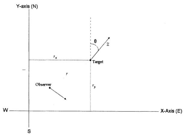
In order to be able to track an enemy submarine or ship, the UUV must be able to perform target motion analysis (TMA). This is the ability to determine the range, course and speed of a target. In order to maintain secrecy, the only information used would be the bearings between the observer and the target, resulting in bearings-only target motion analysis (BO-TMA). The bearing between the observer and the target is the angle at which the observer detects the target (see Figure 1.1). Bearings-only
TMA uses passive sensors, which allows the UUV (or any other vessel) to observe
without being detected itself [30]. This type of underwater TMA has typically been performed by submarines or surface ships performing anti-submarine tactics. The ability to perform TMA with UUVs would allow the UUVs to aquire and track the target sooner than conventional means.
The UUVs could be part of a. sensing network that monitors choke points and delivers information to another vessel that is waiting further out from the choke point,. Figure 1.2 demonstrates the UUV laying out the sensor field as well as tracking a target. The UUV could be cued either by a sensor field or a third party source such as another UUV or a manned vessel. The sensor field might be laid out in advance
Y-axis (N) ~e
z
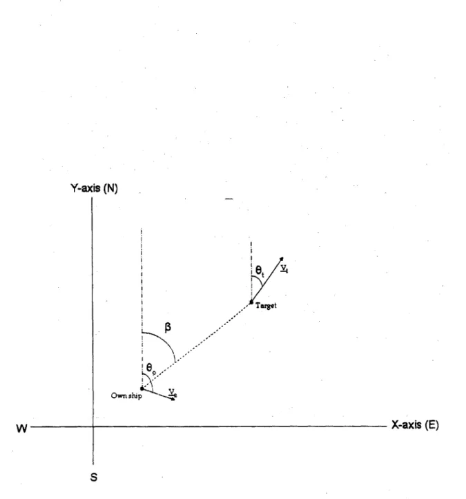
Target V Own ship-d W X-axis (E) SFigure 1.1: Basic geometry definition of bearing between the observer (own ship) and the target. All angles are measured from with respect to 000 as north.
#
is the bearing or line of sight angle between the observer and the target from the point of view of the observer. vt is the velocity of the target (speed and course) while v0 isthe velocity of the observer. 9
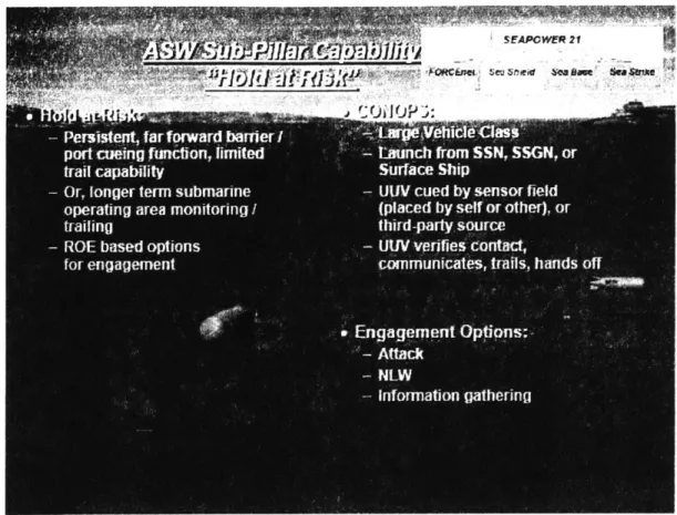
Figure 1.2: Anti-Submarine Warefare Sub-Pillar Concept of Operation "Hold at Risk" from the Navy Unmanned Undersea Vehicle Master Plan [29]
by the same UUV. another UUV. a diver or some other method.
This thesis looks at creating a framework in which to perform bearings-only track-ing with UUVs. In order to do so, some sort of processtrack-ing must be done with the
noisy bearings only data. The different types of ianeuvers that are performed to
accomplish bearings-only tracking are analyzed and used as a starting point to codify
BO-TMA for UUNVs.
1.3
Problem Statement
The fundamental question that this thesis looks at is whether or riot UUVs have the capability to performn BO-TMA without human interaction. Some of the main challenges within this thesis is to develop a proper estiniation algorithm as well as develop a guidance systen for the UUV to perform the required maneuvers to track the target. The estimation algorithm is inherently linked to the guidance svstemr in this application because the guidance system uses the output of the estimation algorithm in making its decisions. This capability is useful because it, allows the UUVs to be iutilized in tracking targets sooner than a manned asset imight, be able to. In order to deterimine whether or not. BO-TMA is feasible using UUVs, an
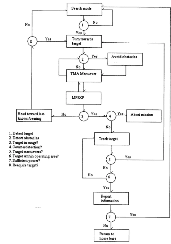
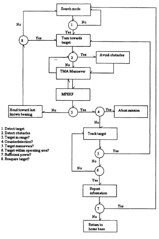
es-timation algorithm was chosen. For the purpose of this research, a modified polar extended Kalman filter was chosen. The reasons for this choice will be further ex-plored in a later chapter. Figure 1.3 presents the proposed flow chart for the control of the vehicle. The chart includes the various aspects of the required mission. In addi-tion to tracking another vessel, the UUV must be aware of its surroundings (avoiding obstacles and avoiding counter-detection) as well as able to complete its mission and report the information that it has gathered to the rest of the area.
The main contributions of this thesis are a working Modified Polar Extended Kalman Filter and a guidance system which allows the UUV to track another vehicle based on sensor information and the surrounding environment.
1.4
Literature Review
The problem of performing and optimizing bearings-only target motion analysis has been extensively studied. There has not been much work with performing BO-TMA with UUVs specifically, but with submarines in general. Much of the work done in target motion analysis was done prior to the major push in work in UUVs in the past ten years. The previous work focused more on the problems of estimation, observability and processing rather than on the actual platform performing the BO-TMA. The work done in bearings-only target motion analysis fall into a few different categories. Typical work has focused on the observability of the problem, what type of estimation to use in processing the data and the optimal observer maneuvers.
The first area in which much work has been done in the bearings-only target motion analysis problem is that of observability. Observability for this problem is defined as the existence of a unique tracking solution [3]. Becker presents both a derivation for a linear approach to the Nth-order dynamics target case [2] and further simplification and application of the observability conditions to more general cases
[3]. Fogel and Gavish also obtained the observability conditions, in which the observer
must have an order of trajectory dynamic greater than that of the target [10]. For example, to observe the trajectory of a constant velocity target, the observer must have some sort of acceleration (either change in course or change in speed). Jauffret and Pillon build on both of these works, examining the nature of observability in passive target motion analysis [15]. For angles-only TMA, a maneuver is required by the observer to obtain observability. The observability problem influences both the choice of estimator as well as the optimal maneuver problem.
A natural extension of the observa-bility problem is to use some form of estimation
algorithm. There are various approaches to this problem: the maximum likelihood estimator (MLE), the pseudo-linear estimator (PLE) and Kalman filters. A fourth approach to the problem is the graphical method, which was commonly used prior to computers and is still taught to submarine officers. Two examples of the graphical method are the Ekelund range and the Spiess range [30]. These were devised by two naval officers in the 1950s and were the first two complete bearings-only TMA solutions.
Searchmode No I No Yes 8 Yes Tu towards target 2 Yes , Avoid obstacles No TMA Manuever MPEKF
Head toward last ,3N Yes ,4 Yes Abort mission
known bearing
No
1. D ete ct target
2. Detect obstacles Track tairget
3. T arget in range? 4. Counter detection? 5. T arget manuevers?
6. Target within operating area? Yes
7. Suffcient power? 8. Reaquire target? N4 P o P 6 Yes Report information 7Yes N No home b as e
estimator is an explicit method which provides solutions as a funtion of the measure-ments [4, 251. However, the PLE has known bias and is not very efficient. Pham presents a quadratic estimator that is similar to the PLE but lacks the bias of the PLE [25]. The PLE is also used in a comparison study of performance against the MLE [22]. Within this study, it is determined that the PLE has increased bias as the effective noise increases, making it an unsuitable estimator for this project.
Nardone, et. al. further explore a closed form solution that is applied in a similar method to the MLE [21]. In Berman's work, a reliable MLE is found that is a hybrid of sorts that works at high ranges [5]. Both the maximum likelihood estimator and the pseudo-linear estimator are nonrecursive batch methods.
These batch methods are compared to recursive methods (which are based in Kalman filtering) [14, 8]. The main difference between the two methods is the method of linearization. The batch processing was determined to be more accurate at ex-tremely long ranges than the recursive processing [14].
The recursive methods consist of the use of Kalman filters. The earliest work in this area developed a Modified Polar Extended Kalman filter (MPEKF) to use in lieu of a regular cartesian Kalman Filter [1]. This modification allows for the state equations to be decoupled and for the measurement to be linear. The modified polar coordinates better reflect the coordinates in which the problem was set. Moorman and Bullock made modifications to the extended Kalman filter to remove most of the bias that was present [20]. All three estimators have been the basis of much of the work done in bearings-only TMA. The MPEKF has advantages in that it uses less processing power. The batch processing of the MLE improves the long range estimation. For the purpose of this thesis, the MPEKF was chosen.
In addition to the work done in observability and estimation, there has also been a focus on optimizing the maneuvers performed by the observer (or own ship). Fawcett used the Cramer-Rao lower bound to predict the behavior of an MLE in response to various maneuvers in order to chose the course that would optimize the performance of the estimator [9]. Passerieux and Van Cappel used optimal control theory to determine the maneuver that minimizes a criterion based on the Fisher information matrix. They determined that [24]
the obtained optimal (or very close to optimal) observer trajectories are as follows: 1) with the range accuracy criterion, a > trajectory with two legs of equal lengths, target near the broadside direction on both legs and direction of the second leg such that bearing rate is maximized, 2) with the global accuracy criterion, a smooth Z trajectory composed of three legs of approximately equal lengths, and 3) in both cases the averaged observer motion is oriented towards the target.
Kronhamn used an adaptive ownship motion control based on the multihypothesis cartesian Kalman filter to determine optimal maneuvers [17]. S.E. Hammel has done much of her work in the area of BO-TMA. Her doctoral thesis focuses specifically on optimal observer motion for the nonlinear tracking problem [13]. Like much of the other work done in this area, it shows that there is a trade-off between increasing bearing rate and decreasing range in the observer maneuvers. LeCadre and Tremois
took a different approach in determining optimal observer motion within bearings-only tracking. They used dynamic programming within a hidden Markov model of the problem [6, 7, 26].
In 2004, the US Navy released its Unmanned Underwea Vehicle Master Plan which was the culmination of many hours of work done by various committees and workshops. It presents an overall view of the current uses of UUVs and a plan for future development [29]. This document presents an overview of the research timelines and areas of necessary development and research. In his master's thesis, Mierisch examined and developed a situational awareness algorithm for UUVs [19]. His basic premise was for the UUV to use its measurements of the contact's motion to determine whether or not it had been detected. Mierisch used probability and known observations of passive and hostile behavior to make this determination.
Another area of work that is vital to bearings-only tracking is that of underwater acoustics. Underwater acoustics provides of the basis of the bearing measurements. Both Lurton and Urick present a comprehensive introdution to underwater acoustics and sound
[18,
28]. Building on Lurton and Urick's work as well as their own practicalexperience, the professors of Underwater Acoustics and Sonar at the United States Naval Academy have created their own set of course notes based on this information
[27]. This work provides the basis for the environmental simulation within this thesis.
1.5
Thesis Organization
This thesis will further delve into the choice and the development of the Modified Polar Extended Kalman Filter in Chapter 2. The guidance algorithm will be pre-sented in Chapter 3, along with its development. Chapter 4 examines the simulation environment and experimental setup. Also, this chapter will further explain the models chosen to represent the underwater environment. Chapter 5 will look at the performance of the algorithm and present. the results of the simulations. The final chapter, Chapter 6, will draw conclusions from these results and present further areas of research.
Chapter 2
Modified Polar Extended Kalman
Filter
There are various approaches to the bearings-only estimation problem. The Modified Polar Extended Kalman Filter (MPEKF) was chosen for this thesis in part due to the commonality of the Kalman filter. The lower processing power and recursive structure required by the MPEKF also makes it a more appropriate candidate for UUVs with limited power. In addition, the proposed situation does not require extreme long range estimation (the area in which the maximum likelihood estimator outperforms the MPEKF). Therefore, this thesis focuses on the use of the MPEKF for its estimation algorithm.
2.1
State Space and Measurement Models
Bearings-only tracking is inherently a nonlinear problem. The nonlinearity can either be in the state equations or in the measurement equations. If a traditional cartesian Kalman filter is used, the state dynamics are linear while the measurement relation-ships are nonlinear. The traditional cartesian state vector consists of the relative position and relative velocity of the target in both the x and y direction.
Transforming the problem into modified polar coordinates, on the other hand, causes the state equations to be nonlinear but the measurement matrix to be linear. The state vector then contains the bearing, the bearing rate, the range rate divided by range and the reciprocal of range of the target from the observer's perspective. The measurement vector has been simplified since it is solely concerned with the bearing. Another benefit of using modified polar coordinates is that the state vector is partially decoupled. The only component that is not observable prior to an observer maneuver is the reciprocal of range. This allows the state estimates to behave as one would theoretically expect, even in the face of errors. unlike the Cartesian coordinates [1].
Y-axis (N) W ~Taget r Observer N X-Axis (E) S
Figure 2.1: Visual representation of the target state vector where r, is the target's x-position, ry is the target's y-position, 9 is the target's course, v is the target's speed and r is the range between the observer and the target.
2.1.1
State space coordinate transformation
Since the algorithm uses the modified polar coordinate system, the transformation from the target and observer state vectors is presented. The initial absolute state space vector for the target is given by
Xt = rxt ryt Vt ot (2.1)
where rxt and r,g are the target position, vt is the target speed and Ot is the target course in cartesian coordinates (Figure 2.1). The state vector for the observer is similar. The modified polar state vector, on the other hand is defined by
Y1
y _ Y2 _ (2.2)
Y3
where r is the range between the observer and the target and 3 is the bearing angle from the observer to the target. The modified polar extended Kalman filter uses the modified polar (MP) state vector for its estimation. However, the information that is of interest to the observer is the course and speed of the target, as well as its position. Therefore, transformations between the two coordinate systems are included within the MPEKF. The cartesian state vector used in Aidala and Hammel's work consists of the relative position and velocity of the target with respect to the observer [1]. The formation of this vector from the aforementioned target state vector is given as
follows:
X1 " vtsin(0t) - vosin (90)
S X2 [vtcos (9t) -vocos (0) (2.3)
3 rXt - rX0
X4 ryt -ryo
where vj is the target's speed, v, is the observer's speed, &t is the target's course, 0, is the observer's course, rxt and ryt are the target's position and rxo and ryo are the observer's position.
Once this state vector is obtained, it can easily be transformed into the y-coordinate system and vice versa. Since the observer state is assumed known with reasonable accuracy, the target information can be pulled from the transformed x state vector. The transformations between the coordinate systems are as follows:
y2sin (y3) + yicos (y3)
X = - Y2cos (y3) - Y1sin (Y3) (2.4)
Y4 sin (y3) [x1X4 - X2x3]/[x + x4] [X1X3 + X2x4] / [x 2 + X 2] y = fy [xix+ -x]/ x4] . (2.5) _ 1/ 2x + X4
2.2
Filter Equations
The filter equations are based on the general discrete time Kalman filter relations from Gelb's Applied Optimal Estimation [12} and the derivation of the MPEKF found in
Tracking [1]. The filter is initialized using
yo
= initial estimate of the MP state vector (2.6) Po = initial estimate of the MP state vector error covariance matrix. (2.7)Once the filter is initialized, the propagation phase commences. This filter does not include any process noise [1]. In the propagation phase between measurements,
= f[y] (2.8)
&f[y]
Ay = f (2.9)
ay
P = A, *P*A . (2.10)
where the function
f
is defined as[S1S4 - S2S3]
/
[S3 + S4] f [Y [S1S3 + S2S4]/ [S3 + S](2.11)
Y3 + tan-1 [S3/S4]]
Y 4/ VS3+ S4 where S1 = y1+y4[wicos(y 3)-W 2sin(y3)] (2.12)S2 = Y2+y41[wsin(y3)+w 2cos(ya)] (2.13)
S3 = (At)yI + y4[w3cos (y3) - w4sin (y3)] (2.14)
S4 = 1 + (At)y2 + y4[wasin (y3) + w4cos (y)] (2.15)
in which wi is relative acceleration term that is dependent on the characteristics of the motion of both the target and observer and At is the time between measurement steps (assumed to be 1 for this thesis). The measurement matrix for this particular EKF is
H = [0, 0,170] (2.16)
because 3 is measured directly.
Using the measurements, the filter estimate is updated using the following equa-tions:
K = P~HT[HP-HT + R] (2.17)
P = [I - KH]P- (2.18)
9 = 9~ + K[z - H -] (2.19)
where R is the measurement noise covariance and z is the actual sensor measurement of bearing 13.
2.3
Observability
Due to the fact that the bearing is the only measurement that the filter is receiving, neither the range nor its reciprical is observable without some sort of maneuver. A passive sensor gives bearing information and possibly frequency information but is unable to obtain range information. An active sensor on the other hand, provides range information since it is known how long it takes the energy to travel to the target and back to the sensor. A passive sensor is just receiving energy. The other parts of the state vector are observable because they can be derived from the bearing measurements. In order for the state vector to be fully observerable, the observer needs to perform some type of maneuver. In this case, the observability of the range is intuitive.
The necessity of an observer maneuver can also been seen by looking at the system dynamics [12]. The A matrix is a partial differentiation of Equation (2.11). This is made up of the S functions given in Equations (2.13) through (2.15). When both the target velocity and the observer velocity are constant, the w terms are equal to zero because the target's and observer's accelerations are zero. If the w terms are equal to zero, the y4 term falls out of the S functions, thereby having no effect on the other states. State y4 = i, so the reciprical of range is not observerable when neither the
target nor the observer have any acceleration. However, when the observer performs a known maneuver, the w terms are now nonzero and y4 will drive 3 (the direct measurement), causing 1 to be observable through 0.
The final method of looking at the observability is to look at it from a linear algebra point of view. In this method, the rank of the observability matrix determines how many states in the state vector are observable [16]. The observability matrix is shown as
H
0 = H A (2.20)
H -A 3
where H is the measurement array given in Equation (2.16) and A is the matrix given in Equation (2.10). During a straight segment of the observer's motion
0 0 1 0
0
[
X 1 0 (2.21)X X 1. 0
where x represents any non-zero value. This matrix has rank(0) = 3 and therefore
is not fully observable. As can be seen by the observability matrix itself, the final column is always zero, indicating that y4 is unobservable. When the observer is in
the middle of a maneuver, the observability matrix is 0 0 1 0
S=
X1 X X X 1X L X1x
(2.22)again where x represents any non-zero value. In this case rank(O) = 4, indicating a fully observable state vector.
All three of the methods demonstrate that a maneuver is required in order to have
a fully observable state vector of the target.
The next chapter will focus on the development of the guidance algorithm and logic through the used of the modified polar extended Kalman filter.
Chapter 3
Guidance algorithm
This chapter looks at the process of developing the guidance algorithm. The various steps building towards the final guidance system include a conceptual flow chart, an examination of the effect of a wide range of maneuvers and the incorporation of the general rule of balancing increasing the bearing rate and decreasing the range, verified
by a detailed maneuver examination, into the final algorithm. Each of these steps will
be further explored in the different sections of this chapter. The guidance algorithm is one of the main contributions of this thesis.
3.1
Guidance concept
Figure 3.1 is a presentation of the conceptual high-level guidance flow chart. This section further examines the guidance components that the flow chart contains.
The initial concept for the guidance begins with the UUV in a search mode, waiting to detect a target or to be cued. This mode allows the UUV to either be in a sweeping mode or a loitering mode. There are two options for the search mode: the
UUV looks for contacts or waits to be cued. When the UUV is looking for contacts, it
will most likely make continuous sweeps of a specified area. An example of this would be to "mow the law" in long paths. On the other hand, a sensor network could have been previously laid. In this scenario, the UUV will loiter until the sensor network alerts it to a coming contact. The sensor network then passes on the target's course, speed and position information to the UUV.
Once the UUV either detects a target or is cued by the sensor network, it turns towards an intercept course with the target. The UUV will either use the information from its own sensors or the information passed from the sensor network to determine the intercept course. Once the UUV has turned towards the target, the bearings-only TMA goes into effect.
Running concurrently with the bearings-only target motion analysis (BO-TMA) is an obstacles avoidance regime. The BO-TMA maneuvers are intertwined with the updates to the Kalman filter, in which both affect the other. Once the maneuvers are complete and the UUV has a good tracking estimate, it falls in behind the target and continues to track it until it either goes out of range, maneuvers, goes out of
Search mode
No 1 No
Yes 1
Yes Turn towards
target 2 2 Yes , Avoid obstacles No, TMA Manuever MPEKF
7.ardlast No 3 Yes 4 yes Abortmission
konearing
No
1. Detect target
2. Detect obstacles Track targeu
-3. Target in range?
4. Counterdetection?
5. Target manuevers?
6. Target within operating ared? Yes
7. Sufficient power? 5 Ye 8. Reaquire target? L o No No6 Yes Report information: 7Yes No Returnto home base
the UUV's operating area or counterdetects the UUV. If the target goes out of range of the UUV's sensors, the UUV attempts to reaquire it. After a specified amount of time, the UUV goes back into serch mode if the target has not been reaquired. Otherwise, if the target is reaquired or if it has maneuvered, the UUV will reenter the BO-TMA mode. If the UUV determines that it has been counterdetected, it will abort the mission, shutting down to minimal power for a certain period of time and wait for a retrieval [19]. This prevents the contact from following the UUV back to its home base. If the contact has left the UUV's operating area, the UUV will report the aquired course, speed and position information to its home platform and return to its search mode. The home platform is the platform from which the
UUV is launched, which could be a ship or a shore station. The UUV can report
the information through a variety of means. Some of these means include using an antennae, or through underwater communication to another UUV or communication buoy. In addition, the UUV can monitor its power availability. If it does not have sufficient power, it will return to its home base to recharge before completing another mission.
3.2
Maneuver scenarios
The development of the guidance logic begins with examining the effectiveness of various maneuvers. An observer maneuver is defined as a course change at a constant
speed for this thesis. These design scenarios vary both the target course and the observer maneuvers. The target course varies between 0 degrees, 15 degrees and 45 degrees. The speed (8 yd/s ~ 14 kts) and the initial absolute starting point (500,500)yds of the target remain constant throughout the various scenarios. The observer also has a constant speed throughout the experiments at a value of 6 yd/s
(~
10 kts). The initial state vector is a transformation of the absolute cartesian states of the observer and target with some added noise. The initial covariance P0 isconstant throughout the trials and is given by [1]:
[ x 10-3rad/s 0 0 0
0 1 X 10⁻³,;-l lxlor= 0 0
o(3.1)
P0
0 1 X 10⁻³rad 0[
0 0 1 x10⁻⁷yd-Ten trials are run within each set-up to allow for the variation in the initial estimate quality. The trials run for 1200 sec each.
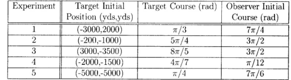
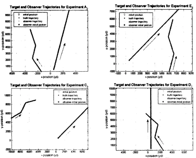
For the most part, the observer performs two maneuvers. The only exception is having the observer begin with a course moving away from the target and performing a 180 degree turn, then performing the normal two maneuvers. The different scenarios include the observer moving away from the target (Fig 3.2 :A 2), moving towards the
target (Fig 3.2 :E 3), long range detection (Fig 3.2 :C3) and short range detection (Fig
3.2 :D 1). The specific parameters of each experiment are presented in Table 3.1.
x-postpon (yd)
Target and Observer Trajectories for Experiment C.
W Zitth trajectory
-bs.O9fr tfajectoly * obhmev milal posntofi
4
Target and Observer Trajectories for Experiment E3
7000
S initial posimon
6MO * lnjth tIaecotry
obseer trjeclory
+ obser initel pestion
2000-1001)
0 "
-1 0D 0 1000 2 0 5 7M0M 8040 9 60
x-posmon fyd)
Target and Observer Trajectories for Experiment D 9020 ac S4001110 initial positiOn 11.1h trajectarv obsever trajeltory
4 obs-ifu Menlt ptiOVIon
-4100 240 60w
x-ri0b0 o (yd)
Figure 3.2: Sample Target Observer Trajectories
Target and Obsirver Trajectories for Experiment A-,
0 initial position
IptAh Iraitctory
- ' bserm I
aietory-+ bse ial pos2on0
EM (O 4( -2(D 0 20M 4CM0 acm cirl 3m0 200 4 10I0O em 40 2000 A im -8 - 0 -I &(N; S= -11%% -~lo EWD -40m 2po sw k30 0CD GO
Experiment Target Observer Ini- Observer Course Change Course tial Position Initial
(rad) (yds,yds) Course (rad)
Turn 1 Turn 2 Turn 3 (rad) (rad) (rad)
A1 0 (2500,200) 37r/16 7r/6 -7/4 0 B1 0 (2500,200) 37/16 -7r/6 7r/4 0 C1 0 (2500.200) 37r/16 -57/12 r/3 0 D, 0 (2500,200) -37/16 7r/4 -7/3 0 E, 0 (-1500,200) -37r/16 r/4 -7r/6 0 A2 7r/12 (-1500,200) -37r/16 7r/4 -7r/6 0 B2 7r/12 (-1500,200) 0 7r/4 -7r/6 0 C2 Tr/12 (2700,200) 7r/4 -37r/8 7r/3 0 D2 7r/12 (2700,200) 37r/16 7r/6 -77r/16 0 E2 7r/12 (2700,200) 37r/4 -7 r/6 -7/3 A3 r/4 (200,2500) </12 </3 -27r/9 0 B3 7/4 (-1500,200) r/16 r/4 -7/3 0 C3 7r/4 (-10000,5000) 7r/3 -7/6 /4 0 D3 r/4 (6000,-1000) -7/6 7/2 -7/4 0 E3 7/4 (6000,-1000) 7r/12 -7/6 r/6 0
Average Course Error (Magnitude)
Over 10 trials for target angle 0
Experiment A Experiment B -uever Experiment C Experiment D Experi 2nd Manuever - - -200 400 600 800 Time in simulation 1000 1200 1400
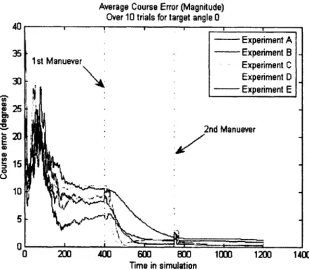
Figure 3.3: Course Error results for the set of experiments that include a target course of 0 degrees
and estimated trajectories. This is one of the areas in which the effectiveness of the maneuver is determined. Using the different parameters, various aspects and effects of the maneuvers are analyzed both qualitatively and quantitatively. For a purely qualitative analysis, the visual results of the estimated and actual trajectories are used.
For each trial and each experiment, the initial guess of the y state vector is varied from truth by a random number. The initial visualization of the results allows for a basic analysis of the effectiveness of the maneuver. The estimation often goes from having erratic behavior to a bit more consistent behavior after the first maneuver is performed (as expected). Even in cases where there are large initial errors, the maneuver brings the estimation closer to the actual course of the target.
In addition to a qualitative analysis, a quantitative analysis is performed. This quantitative analysis takes the average of the ten trials for each experiment. The initial estimatation error varies over the trials due to the random error that was added to the actual value of the state vector. Three different metrics are evaluated in each run: the error in the course estimation, the error in the speed estimation and the error in the range estimation. The calculation of the averages uses the absolute values of the errors, since the magnitude of the error provided more information than the sign of the error. An example of the results can be seen in Figures 3.3, 3.4 and
3.5.
These figures also plot the time of the maneuvers. In each of the metrics, the maneuver has an effect on the results. In both the course and speed, the error estimate levels out prior to the maneuver to a steady error. However, after the maneuver, the
40 351
I
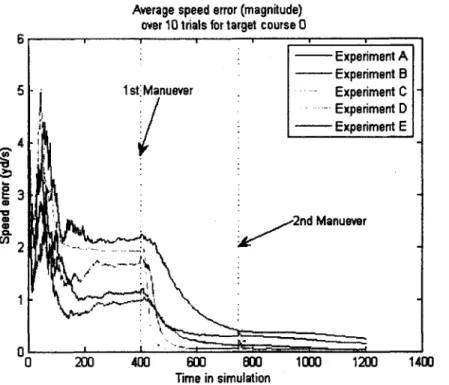
1st Man 30 i ~2S o20 0) 10 15 0 10 5 01 0 ment EAverage speed error (magnitude)
over 10 trials for target course 0
5 4 3 0 0 200 400 600 800 Time in simulation 1000 1200 1400
Figure 3.4: Speed Error results for the set of experiments that include of 0 degrees
a target course
E A
Average range error (magnitude) over 10 trials for target course 0
1st Manuever AVp Exper Experi Experi Experi -
:1
-' 2nd ManueverL~
200 400 600 800 1000 1200 1400 Time in simulationFigure 3.5: Range Error results for the set of experiments that include a target course of 0 degrees Experiment A Experiment B mentC -ment D ment E - 1st Manuever Experi Experi Experi 2nd Manuever 2000 1500 1000 500 ment A ment B ment C ment D ment E 0 a) 0 0 I I
error decreases in all three metrics. In general, the range error tends to rise prior to the observer's maneuver. The only exception in these 5 experiments is experiment
D. In this case, the range error initially decreases rather than increases, due to the
fact that its initial course is directed towards the target rather than away from it. The general rise in range error is the expected result since the state that. includes the range is unobservable prior to a maneuver. All five of the experiments result in a. decrease in the error after the first maneuver, however the steepness of that decrease varies. The quicker the drop, the more effective the maneuver. This is true within all three metrics. As can be seen in Figures 3.3, 3.4 and 3.5, experiments C and D have the most significant drops in error after the maneuver. They also have the smallest errors at the end of the run. Since these results look at the averages over ten trials,
some of the large errors that occur in individual trials are smoothed out.
An observation from these experiments is that the observer's motion should gen-erally be towards the target. The results of these experiments confirm the generalized rules for optimal observer maneuvers found in the literature [24]. In general, one wants to find a balance between
" increasing the bearing rate and
" decreasing the range [4].
The maneuvers that did better tend more towards the target than away from the target. Another observation from these experiments is that the initial estimate needed to be tweaked a bit. The initial estimate is based on the actual state values with some random error added to it. The issue develops for the long range scenarios since the error is added into the y state vector. In this state vector, one of the states is the reciprocal of range. For long range scenarios, the same error creates a much greater initial error since the magnitude of the error added to the state was greater than that of the state itself. In order to overcome this in the final runs, the error is added to the x state vector prior to it being transformed into y space. This change is also consistent with the scenario in which the x state vector is the information given to the UUV by the sensor network that has cued it. It is assumed that there is an initial error in the information that passed to the UUV, rather than perfect information.
3.3
Guidance logic
The guidance logic takes various factors into account. The variables that are fed into the logic include the observer's current state, the target's estimated state, the estimated y state vector, the detection of the target, the current observer course com-mand, the future course commands, the length of an individual leg of the maneuver and the current BO-TMA command. The main output is the course command for the observer.
The first part of the guidance logic calculates a good intercept course based on the relative positions of the target, and observer as well as the target's estimated course. The goal of this logic is to calculate a course that will allow the observer to come
within range of the target. In order to do so, the observer's course must be in the direction of a point ahead of the target's current position. In order to achieve this point, the command course is chosen to be either perpindicular to, 45 degrees off of or 15 degrees off of the target's estimated course based on the relative positions of the observer and target. If the observer course is close to parallel to the estimated bearing between it and the target, its course remains constant. Otherwise, the observer turns towards the target's course.
Once the target is within range of the observer, the guidance calculates the BO-TMA maneuver. The basis of this maneuver are the guidelines presented in the literature that have been verified within this thesis. The maneuvers follow a basic Z pattern as described in Passerieux and Van Cappel's work [24]. The guidance logic calculates the two different courses the observer needs to take. The general direction of the maneuver is always towards the target. In each of the following cases, the third leg of the maneuver is the same as the first leg of the maneuver.
* If the observer's course is within 15 degrees of the target's estimated course
- The first leg of the maneuver is the observer's current course
- The second leg of the maneuver turns towards the target with a course that is 30 degrees off of the target's estimated course
* If the observer's course is close to being the reciprocal' of the target's estimated course
- The first leg of the maneuver is the target's estimated course
- The second leg of the maneuver turns towards the target with a course that is 30 degrees off of the target's estimated course
" If the observer's course is towards the target
- The first leg of the maneuver is the observer's current course
- The second leg of the maneuver is the target's estimated course * If the observer's course is away from the target
- The first leg of the maneuver is the target's estimated course
- The second leg of the maneuver turns towards the target with a course that is 30 degrees off of the target's estimated course
The guidance algorithm allows the maneuver to complete, even if the target is out of range of the observer. Once the maneuver is complete, the observer will either come to a course parallel to the target's estimate or it will turn around, indicating that the target has moved outside the range of the observer. However, this does not happen immediately but rather after a specified amount of time has elapsed.
The guidance logic also keeps track of the history of the target state estimations. The history provides the metric to determine whether or not another maneuver is required. One of the basic assumptions for this problem is that the target has a constant course and speed. Within the estimation, small variations are expected. However, if there is a large jump within either the course or the speed history, a new maneuver is required to maintain the integrity of the estimation. Once this is determined, the guidance algorithm will calculated another set of maneuvers.
If the target leaves the range of the observer's sensors, the observer continues on
its current course for a specified time in order to try to reaquire the target. If the observer does not reaquire the target, it turns away from the last known position of the target and returns to its home base. In the simulation, this is represented by a
180 degree turn.
The guidance logic is incorporated into the main control of the UUV. The next chapter will explore the environmental model and simulation set-up.
Chapter 4
Simulation and Environment
Models
This chapter explores the environmental and the simulation models. The underwater environment is a tough environment to model. This chapter presents the various simplifications and assumptions made in the final simulations. After exploring the sensor detection radius and environment, this chapter will present the set up for the various trials used to test the guidance algorithm.
4.1
Detection Algorithm
The detection algorithm determines whether or not the target is within the range of the passive sonar. If the range of the sonar extends past the location of the target, then the target is detected. A sonar range algorithm is used in conjunction with the detection algorithm.
The range in which a target. can be detected depends on various factors and parameters. For passive sonar. these factors are the target source level (SL), the ambient and self-noise level (NL), the transmission loss
(TL).
the detection threshold (DT) and the receiving directivity index (DI) [28, 271. These parameters are combined in the passive sonar equation:SL - T L - AIL + DI ;> DT ,(4.1)
expressed in dB. The range at which a target is likely to be detected can be estimated
by solving for the transmission loss at a specific detection threshold:
r.
TL = 20logi0ro + 10log,1 - + a (r x 1() (4.2)
where r-0 is the transition range between spherical and cylindrical spreading and a is the attenuation coefficient. In order to simplify the calculations, the transmission loss due to attenuation is assumed to be very small. It is also assumed that the transmission loss is due to spherical spreading and the effects of cylindrical spreading
are ignored. This results in
TL ~~ 10loglor (4.3)
being the function used to calculate the range of the sonar. This relation is a simplified version of a more detailed model and does not take into account all of the aspects of the environment. However, the purpose of this exercise is to have a way to model the range of the sonar in the scenario with some basis in reality rather than picking
a number out of thin air.
The detection threshold is the point at which the system determines that there is a contact. This threshold is based on the detection index desired for the sonar, as well as the bandwidth and integration time of the sonar. The detection index is pulled off of a chart based on the desired probability of detection, p(D), and probability of a false alarm, p(FA):
DT = 5og10o ( (4.4)
where d is the detection index, T is the integration time and
6f
is the bandwidth frequency of the sensor.The directivity index, detection threshold and the self-noise are all parameters based on the sonar equipment. The directivity index depends on the type of array used as well as the frequency of the sound wave. There are many different estimations of the directivity index, depending on the shape of the array. For this thesis, the sonar was assumed to be a conformal array, with a DI of 19.54 dB at broadside [11]. For the purpose of these calculations, the directivity index was assumed to be constant thoughout the entire scenario. The transmission loss and the ambient noise level depend on the environment that the observer is in. The noise level in the passive sonar equation includes the self-noise and the ambient noise of the environment:
NLamb = NL8, E NLship (4.5)
NLto=N Lamb E NLself (4.6)
where E represents the power sum of two decibel quantities:
L1 e L2 = 1-010 10 (100 + 100. (4.7)
The source level is the level of noise radiated by the target [18, 27, 28]. Of these parameters, only the transmission loss is unknown. The sonar parameters are modeled based on known literature. Within this thesis, two environments will be modeled through the use of varying the ambient noise level for different conditions. The source level of the target can also be modeled for various targets. This variation is important because it allows for the effectiveness of the algorithm to be evaluated in different situations.
The model of the source level of the target used and modified old data from World
War II era submarines [18, 28]. It is assumed that all current data is classified, but, that the presented model can easily be adjusted for proper parameters.
algo-rithm can determine whether or not the UUV can "hear" the target. This algoalgo-rithm is used both in initiating the bearings only tracking as well as maintaining the track of the target.
4.2
Environment
Target motion analysis and target tracking are common activities in blue water en-vironments. Blue water environments are also known as open ocean or those waters that lay beyond the coastal regions of the earth [23]. A key benefit of using UUVs is to perform this mission within a littoral area. The littoral area is that area that is closest to shore (within 600 feet of the shoreline) [23]. The UUV would be able to penetrate closer to harbors and choke points than would a manned sub, effectively becoming a force multiplier. The effects of the environment are simulated within the passive sonar equation in the detection algorithm.
For the purpose of this thesis, two different scenarios are created. Their specific parameters are presented in Table 4.1. Both occur in shallow water environments. The two aspects of the ambient noise are due to shipping and to the sea state. The two different scenarios represent a typical day (refered to as the nominal case) and a worse case scenario type of day. For the typical day, the shipping is assumed to be heavy since the UUV would be acting either just outside a harbor or a choke point. The sea state is assumed to be 1, with a wind speed of four to six knots. For the worst case scenario, the sea state is assumed to be 6, the highest sea state with wind speeds of 28 to 33 knots. Since it is a very heavy sea state, the shipping levels are assumed to be moderate.
Wenz curves are used in order to convert this information into the decibel form that is required for the passive sonar equation [18, 27, 28]. Figure 4.1 is a simplified version of the Wenz curves that was used to determine the noise levels due to shipping and sea state. The value is found at the intersection of the shipping or sea state with the center frequency of the bandwidth. The center frequency is found by taking the geometric mean of the two end frequencies of the bandwidth.
Parameter Environment 1: Nominal Case Environment 2: Worst Case Self noise (NL,ef) 50 dB 50 dB
Source level (SL) 110 dB 110 dB
p(D) .90 .90
p (FA) .002 .002
Bandwidth (Af) 400 Hz 400 Hz Integration time (T) 20 ins 20 ms
Sea state 1 6
NLS 81 dB 99 dB
Shipping heavy moderate
NLesh 93 dB 80 dB
![Figure 4.1: Simplified Wenz Curve [27]](https://thumb-eu.123doks.com/thumbv2/123doknet/14148374.471507/40.918.104.781.114.521/figure-simplified-wenz-curve.webp)