Analysis of the impact of collaborative ground delay programs in air traffic control

ANALYSIS OF THE IMPACT OF

COLLABORATIVE GROUND DELAY

PROGRAMS IN AIR TRAFFIC CONTROL

by John R. Jensen

Submitted to the Department of Civil and Environmental Engineering in Partial Fulfillment of the Requirements for the

Degree of

Master of Science in Transportation at the

Massachusetts Institute of Technology February 1999

© Massachusetts Institute of Technology All rights reserved

A uthor...--... ... --- --...

Department of Civil and Environmental Engineering January 26, 1999

Certified by...---. ... --- .---.--- . --... Amedeo R. Odoni T. Wilson Professor Department of Aeronautics and Astronautics and Civil and Environmental Engineering

Accepted by ...---... .. ;: .And--- h---AndrewJ. Whittle Chairman, Departmental Committee on Graduate Studies

ANALYSIS OF THE IMPACT OF

COLLABORATIVE GROUND DELAY

PROGRAMS IN AIR TRAFFIC CONTROL

by John R. Jensen

Submitted to the Department of Civil and Environmental Engineering on January 26, 1999, in partial fulfillment of the requirements for the Degree of

Master of Science in Transportation

Abstract

Ground delay programs (GDPs) have been a pervasive feature in U.S. air traffic management for many years. Recently, an enhanced version of the ground delay programs has been instituted as part of collaborative decision making, a new approach to air traffic management. This enhanced versions holds out the promise of improving the system by making better use of the scarce resources during capacity-constrained operations, and by giving the airlines greater flexibility in managing their flights. Prototype operations of the enhanced program went into effect on January 2 3rd at two airports, and was subsequently extended to two additional airports on April 28th. This thesis analyzes and evaluates the information collected from the first nine months of prototype operations.

A computational analysis model has been developed to analyze the effects of the enhanced GDPs. The model uses information about flights arriving at airports under prototype operation and about the GDP programs themselves. The model extracts the critical pieces of information, and organizes this information in a database. This database is then used as the basis for all subsequent analysis. The model has been used to analyze the incidence of GDPs, ground hold delay savings gained by airline flight substitutions and GDP compression, capacity utilization during restricted operations, unexpected airborne holding, airborne delays during GDPs, and the increase in flight cancellations due to GDPs.

Thesis Advisor: Dr. Amedeo R. Odoni

Title: T. Wilson Professor of Aeronautics and Astronautics and Civil and Environmental Engineering

Dedication

This study is dedicated to MJ, my wife, and to Mark and Todd, our two sons. Without their love and support over the years, I would never have been able to engage in my studies at M.I.T. I owe them a debt of gratitude, especially for their endless patience and understanding over the last ten months, when I would frequently absent myself to work on this study.

Acknowledgements

I am grateful for the support of the Federal Aviation Administration, which funded the research for this thesis.

I am especially indebted to professor Amedeo Odoni, who suggested I work on this study. His constant prodding and probing questions often induced me to reevaluate my line of thinking and explore new avenues, gaining a new understanding of and a better appreciation for the complexities of the subject along the way.

I would also like to thank Joe Sussman, Cynthia Barnhart and Carl Martland in the Center for Transportation Studies, and John Hansman and Peter Belobaba in the Department of Aeronautics and Astronautics. I have enjoyed their teachings and their wisdom over the last

six years more than I can say in words.

I have had the opportunity to meet many gifted people and make many new friends during my stay at M.I.T. They are a big part of why I have found this time to be such an enjoyable and learning experience.

TABLE OF CONTENTS

1 Introduction ... 7

1.1 B ackground... 7

1.2 O verview of content... 11

2 R esults ... 13

2.1 T erm inology used ... 13

2.2 Incidence of G round D elay Program s ... 14

2.3 Substitution and Com pression A nalysis... 20

2.4 A rrival Slot Utilization... 30

2.5 U nexpected A irborne H olding... 40

2.6 A irborne delay ... 49

2.7 Cancellations... 68

3 Conclusions and Suggestions for Further Analysis and Research ... 73

3.1 Conclusions ... 73

3.2 Suggestions for further analysis and research ... 77

A A cronym s ... 85

B Com putational A nalysis M odel... 86

B .1 O verview and Environm ent... 86

B .2 Flight D ata Extraction... 89

B .3 G D P Program Param eters... 91

B .4 D atabase Processing... 92

A .5 Q uerying the database... 96

A .6 Finalizing the results ... 100

C D atabase Tables and File Form ats...102

C .1 D atabase tables... 102

C .2 File Form ats... 104

C .3 Program s...108

LIST OF TABLES

Table 2-1: G round delay program s ... 15

Table 2-2: SFO average scheduled arrivals and active-GDP AARs ... 17

Table 2-3: Airline substitution and GDP compression summary results ... 22

Table 2-4: Flown flights that were at some point affected by GDP... 23

Table 2-5: SFO average delay and delay savings per GDP flight, by month... 25

Table 2-6: Adjusted arrival capacity (AAR') example ... 32

Table 2-7: SFO slot utilization, by hour... 33

T able 2-8: SFO capacity analysis... 36

Table 2-9: Average unexpected airborne holding, by month... 42

Table 2-10: STL Unexpected airborne holding for 4/28, 4/29, 5/15 and 5/22... 44

Table 2-11: STL hourly AAR and unexpected airborne holding on 4/29... 44

Table 2-12: STL hourly AAR and unexpected airborne holding on 5/22... 44

Table 2-13: Unexpected airborne holding variance at EWR and SFO ... 46

Table 2-14: Comparing the unexpected airborne holding means statistically ... 47

Table 2-15: Average airborne delay per flight, by month ... 51

Table 2-16: SFO average airborne delay per flight, by month ... 52

Table 2-17: EWR average airborne delay per flight, by month... 54

Table 2-18: Average airborne delay, by destination... 60

Table 2-19: SFO mean airborne delay test results for six airports... 61

Table 2-20: SFO average airborne delay test results, by GDP state ... 65

Table 2-21: Average airborne delay, by destination... 65

Table 2-22: Airborne delay statistical comparisons, by GDP state... 67

Table 2-23: Airborne delay statistical comparisons, by destination ... 68

Table 2-24: Average daily cancellations for GDP and non-GDP days ... 69

Table 2-25: Testing increases in cancelletion on days with GDPs ... 70

Table B-1: Scheduled number of flights at 12 airports for one day (9/30/98) ... 94

T able B -2: File size com parison... 96

Table B-3: comprep example output (partial results from 'comprep sfo 19980930')... 97

Table B-4: aarrep example output (partial results from 'aarrep sfo 19980930')... 98

Table B-5: abhrep example output (partial results from 'abhrep -g etatz sfo 19980930') ... 99

Table B-6: eterep example output (partial results from 'perl eterep') ... 100

T able C -1: flights table definition ... 102

T able C -2: A A R table definition ... 103

T able C -3: G D P table definition ... 103

T able C -4: G dpevent table definition ... 103

T able C -5: A irport table definition ... 103

Table C-6: ADL file format (arrivals section) ... 105

T able C -7: Slot assignm ent file form at...105

Table C-8: flight and flight.db2 file form at...106

T able C -9: gdp.event file form at...107

T able C -10: G D P event types... 107

T able C -11: G D P .db2 file form at...108

T able C -12: gdpevent.db2 file form at... 108

LIST OF FIGURES

Figure 1-1: C om pression exam ple... 10

Figure 2-1: G round delay program s ... 16

Figure 2-2: SFO incidences of G DPs, by hour... 17

Figure 2-3: SFO average scheduled arrivals and active-GDP AARs, by hour ... 18

Figure 2-4: SFO quarterly incidences of GDPs, by hour ... 19

Figure 2-5: EWR quarterly incidences of GDPs, by hour... 19

Figure 2-6: Flown flights affected at some point by GDP ... 24

Figure 2-7: SFO substitution and compression savings per GDP flight, by month... 25

Figure 2-8: SFO number of CTA changes, by hour... 27

Figure 2-9: SFO ground delay, by hour ... 27

Figure 2-10: EWR number of CTA changes, by hour ... 29

Figure 2-11: EW R ground delay, by hour... 29

Figure 2-12: SFO average net matching of slots to demand, by hour... 34

Figure 2-13: SFO average active-GDP matching of slots with demand... 35

Figure 2-14: SFO fraction of days where AAR capacity is sufficient to handle actual arrivals . 37 Figure 2-15: SFO average quarterly matching of slots with demand, by hour... 38

Figure 2-16: SF0 average recovered slots from a cancelled GDP ... 39

Figure 2-17: Average unexpected airborne holding for GDP and non-GDP flights ... 42

Figure 2-18: Average unexpected airborne holding for active-GDP flights... 43

Figure 2-19: SF0 average monthly UABH, by type of GDP flight... 46

Figure 2-20: SF0 average monthly UABH, by type of GDP flight... 48

Figure 2-21: Average airborne delay per flight, by month... 51

Figure 2-22: SFO average airborne delay per flight, by month... 52

Figure 2-23: EWR average airborne delay per flight, by month ... 53

Figure 2-24: Average airborne time delay, by destination... 55

Figure 2-25: SFO scheduled vs actual airborne time on 9/1 (non-GDP) and 9/30 (GDP) ... 56

Figure 2-26: SFO number of scheduled flights versus actual flights for six origins ... 57

Figure 2-27: SFO airborne time distribution for six origins ... 58

Figure 2-28: SF0 airborne delay distribution for six origins ... 59

Figure 2-29: SFO relative airborne delay distribution for six airports... 59

Figure 2-30: SEA-SFO scheduled and actual airborne time, by GDP state ... 62

Figure 2-31: SEA-SFO airborne delay, by GDP state ... 62

Figure 2-32: ORD-SFO airborne delay, by GDP state ... 64

Figure 2-33: Cumulative arrival percent by relative airborne delay, by GDP state... 66

Figure 2-34: Cumulative arrival percent by airborne delay, by destination ... 66

Figure 2-35: Correlating number of cancellations to average GDP delay ... 70

Figure 2-36: Correlating cancellations to average GDP savings from subs and compression .. 71

1 Introduction 1.1 Background

Ground delay programs (GDPs) have long been a feature in the management of the U.S. airspace. They are designed to manage operations at an airport, when arrival demand is projected to exceed the available capacity for a substantial amount of time. GDPs work by pre-assigning a specific, controlled time of arrival (CTA) to a flight, and then reserving the arrival slot for that flight. Since the flight time between the origin and destination airport can be determined with reasonable precision, this also determines a controlled time of departure (CTD). The flight is then held on the ground at the originating airport until the CTD time. At that time, it can depart, with the assurance of being able to proceed to the arrival airport and being able to land with a minimal amount of unexpected airborne holding (UABI-H).

When working properly, GDPs have two major benefits. First, they increase the overall level of safety in the system by reducing the number of airplanes present in the terminal airspace of an airport. Since each airplane has a specific arrival time assigned to it, it will spend less time in airborne holding and hence in the terminal airspace. Second, there is a substantial gain in economic efficiency to the airlines operating the flights. Since delays are incurred on the ground rather than while aloft, fuel is not used. Fuel consumption is a major expense item for all airlines, so reducing the airborne holding directly reduces the amount of fuel spent to complete the trip.

The GDP process starts when the FAA determines the arrival acceptance rate (AAR) in response to current or foreseen reductions in airport capacity. This reduction may be caused by inclement weather, airport construction, or special runway operations. The AAR specifies how many flights the airport is projected to be able to handle for each given hour. AARs for several consecutive hours are typically defined at the same time.

A critical element in GDPs is the allocation and distribution of arrival slots. In the past, an algorithm known as the Grover-Jack algorithm has been used to perform this task. It allocates the available arrival slots at an airport according to the estimated time of arrival (ETA) of the

1 This section is heavily indebted to the discussion of this subject found in [1]. For a more detailed discussion, please refer to this paper.

incoming flights. The algorithm preserves the order of the original set of flights, but stretches out the arrivals in time to make the number of arrivals within each controlled hour stay within the available capacity at the airport, as defined by the AARs. It also has to factor in slots for flights that are exempt from the GDPs. Flights can be exempt for a number of reasons. International flights, general aviation flights and flights already airborne are exempt and cannot be issued a ground delay. Other categories may also be classified as exempt, such as flights originating at airports where de-icing is in effect.

Since Grover-Jack uses the flight ETAs as its means of rank ordering the set of flights to be controlled, any delay caused within an airline for a particular flight may end up resulting in a double penalty for that flight. This happens if the flight, after being delayed by the airline itself, is subsequently subjected to the Grover-Jack algorithm. This has caused some concern within the airline industry, and has acted as a disincentive for submitting updated ETAs to the FAA. This issue has been one of the factors driving the exploration of new ways to address the scheduling of flights into capacity-constrained airports.

Collaborative decision making (CDM) is a key component in the larger concept of the National Airspace System plan known as Free Flight. Its key goal it to seek a new way of ensuring that the airspace is used in a safe manner, while at the same time turning over more decision making responsibilities to the users of the system.

A CDM working group has been formed to steer the activities underway in this area. New algorithms for air traffic management have been developed, and a communications infrastructure has been established to ensure that the FAA and participating airlines have a common view of the arrival demand picture at every U.S. airport. Prototype operations of GDP-E (Ground Delay Program - Enhanced) under the CDM Program commenced at San Francisco (SFO) and Newark (EWR) on January 2 3rd, and were extended to La Guardia airport, New York (LGA) and St. Louis, Missouri (STL) on April 28"'. GDP-E was subsequently extended to all major U.S. airports on September 8'.

A new computer network was set up as part of CDM to facilitate the flow on information between the airlines and the FAA. Named the AOCnet (Airline Operations Center network), it connects the participating airlines' operations centers with the FAA Air Traffic Control

System Command Center (ATCSCC) and the CDM hub-site at the Volpe National Transportation System Center (NTSC). Every five minutes aggregate demand lists (ADLs) are distributed across this network to the airlines. These lists contain the current status information of all flights in the system. The intent is for this information to be used by the airlines to facilitate them in their scheduling decisions. A computer application, the Flight Schedule Monitor (FSM), has been developed as part of CDM. FSM makes direct use of the ADL information, and enables its users to analyze the impact of alternative scheduling

strategies before deciding upon which course of action to pursue.

A new arrival slot allocation algorithm named Ration by Schedule (RBS) has been developed as part of the CDM effort. As the name of the algorithm implies, arrival slot allocation is now being governed by the scheduled time of arrival, as opposed to the estimated time of arrival. Any delays internal to the airline companies do not influence the GDP arrival slot allocation process. This means that there no longer is an incentive for the airlines to withhold flight ETA updates, leading to a more accurate picture of the overall state of the system.

The airlines still maintain the ability to substitute flights within the pool of arrival slots allocated to them. This enables the airlines to swap an arrival slot allocation of one flight for another, moving up one flight in time and another back in time. It furthermore allows the airlines to cancel a flight and move another one up to take the place of the cancelled flight.

The RBS algorithm helps allocate the available arrival slot resources among the airlines. It does not, however, address the issue of what to do when an airline cannot make use of an allocated slot. This situation occurs when a flight is cancelled or moved up in time to an earlier slot, and the airline has no other flight that can be moved to take over the abandoned arrival slot. The compression algorithm has been developed to address the issue of allocated slots going unused. In simple terms, it does this by filling up any unusable slots with later-arriving flights, moving up flights to fill up the available slots as much as possible. The compression will respect the original rank ordering of the flights, while at the same time ensuring that a flight is

not scheduled any earlier than its earliest possible arrival time.

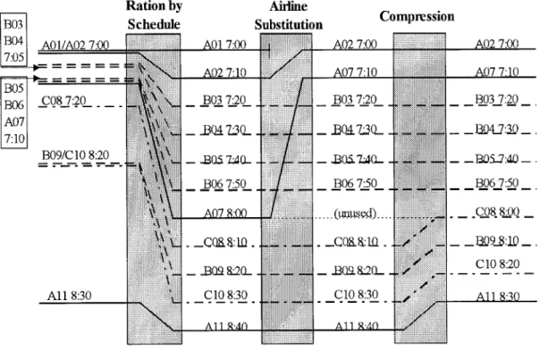
An example may help illustrate the three interrelated concepts of ration by schedule, airline substitutions and compression. The example is borrowed from [1], but its graphical form

given in figure 1-1 is new. In the example, 11 flights (01 through 11) from three different airlines (A,B,C) are scheduled to arrive between 7:00 and 8:30. Due to capacity restrictions at the airport, only one flight may land every 10 minutes. This arrival rate is admittedly unrealistic, and is used here only to make the exposition clearer. The initial situation is depicted to the left in Figure 1-1. Time of actions move from left to right in the figure.

B03 B04 _{AO1/A02 7:00} 7:05 __ B05 B06 C08 7:20 -A07 7:10 B09C10 8:20 All 8:30 Ration by Schedule AOl 7:00 A02 7:10 \.. _.. B03 7:20 S- _O5 7,40-. A \ B06 7:50 \ 302a &2 \ -C1O 8:30 A1 I-4 I Airline Substitution C A02 7:00 A07 7:10 B03 7:20 J30A7._3Q-2057.40-. B06 7:50 .(sed) .B09.820_ . _ClO 8:30 Al11 R-4n ompression A02 7:00 A07 7:10 B03 7:20 .B05-740-_B_06 7:5_ C08 8:00 C0 8:20 . _ _A l_.._8:3_..__

Figure 1-1: Compression example

Flights A01 through All are scheduled to arrive at the airport between 7:00 and 8:30. Due to an inability to handle more than six flights per hour, the RBS algorithm is run to reschedule the arrivals. This results in the arrival line-up shown to the right of the Ration by Schedule semi-transparent box. Overall, a total delay of 320 minutes is allocated, spread out over the airlines by 70 minutes to A, 150 minutes to B and 100 minutes to C. These delays are computed by calculating the delay for each individual flight as the difference between the scheduled and RBS-allocated arrival times.

After the initial RBS allocation has been completed, and the resulting arrival slot allocations broadcast to the airlines, they have a chance to substitute flights in the slots that have been assigned to them. These actions are shown in the airine substitutions box. In the example, flight

A01 is cancelled, flight A02 is moved up to take over A01's slot, and flight A07 is moved up in the now-vacated slot of flight A02. This leaves the slot at 8:00 unused. Airline A does not have any flights that can be moved into this slot, since its only other arriving flight has an earliest arrival time of 8:30, well after the 8:00 opening. Airlines B and C have flights that can move into this slot, but they cannot do so, since the slot is owned by A. Airline A is the only one to perform any substitutions, so it is the only one to see any change in its overall delay. Its delay drops from 70 minutes to 10 minutes, for overall savings of 60 minutes, but at the cost of having one flight cancelled. System-wide there is the same 60 minutes of savings, for a revised total delay of 260 minutes.

Finally, compression is run. The effects of this are shown in the compression box. In the example, each of the four last flights is moved up by one slot, in the process clearing out the unused slot. This results in an additional 40 minutes saved system-wide, with 10 minutes going to A, 10 minutes to B and 20 minutes to C. Overall, the delay is now 0 minutes for A (but with one cancelled flight), 140 minutes for B and 80 minutes for C. The total of 220 minutes of delay is the best that can be achieved on a system-wide basis.

1.2 Overview of content

An early assessment of CDM is described in the report issued by NEXTOR entitled Collaborative Decision Making in Air Trafic Management: A Preiminay Assessment [1]. This report dealt with several different topics related to CDM, analyzing the changes in the quality of the information, the impact of the distribution of information and the increased situational awareness that this has brought about, the ability of the airlines to make economic resource allocation decisions, and some of the delay reductions and other benefits associated with CDM-based ground delay programs.

The objective of this study is to continue the investigation started in [1], and to build a computational framework that will facilitate future work in this area. The study evaluates some of the effects of the first nine months of prototype GDP-E operations. A more detailed assessment has been made of the ability of CDM to reduce the GDP delays through airline substitutions and GDP compression. Capacity utilization has been reviewed to determine how fully the stated AAR capacity is being utilized, and if there are any signs of systematic or periodic under-utilization. The analysis on airborne holding started in [1] has been extended to

cover additional airports and more dates. An investigation has been carried out to evaluate the impact of GDPs on airborne delays. Finally, cancellations have been investigated to determine if the overall number of cancellations increases on GDP days, and whether or not there is a correlation between the FAA arrival slot allocation delay and the number of flights being cancelled.

The data used for this study come from two sources. The first source is the AADL files. These files are organized by destination airport, with one file per airport. Each file contains information about all flights arriving at a given airport on any particular day. To limit the size of these files, only flight records that show one or more changes in their content fields from the previous record have been retained. Datafiles for the entire nine months and the four prototype airports have been made available for use within this study. The second source of data covers the GDP control information. This information has been retrieved from a Metron web-site. These two databases have been processed through a series of computational steps to create a database of flight-level information. This database has then served as the data-source for all the analysis work conducted as part of this study.

Chapter 0 describes the results of the analyses that have been performed on the data. The specific areas covered are ground delay programs, compression results, arrival slot utilization, unexpected airborne holding, airborne delay, and cancellations. Chapter 3 summarizes a set of conclusions, and offers many suggestions for further analysis that may be warranted and useful. A series of appendices provide additional details on the computational model. Appendix A contains a list of acronyms used throughout. Appendix B describes the computational model that has been built to help evaluate the large amounts of data being collected. It deals with the issues of collecting and reducing the flight data to a manageable level, collecting the GDP control information, setting up a database to manage this information, and finally extracting the information from this database to provide a basis for analysis. Appendix C provides reference information for the model, i.e., definitions of the database tables, file formats and computer programs used.

2 Results

This study looks at various indicators of performance during the first nine months of prototype operations of GDP-E. In the sections that follow, a number of aspects are examined: ground delay program statistics; effects of GDP compressions; slot utilization; unexpected airborne holding; en-route delays; and cancellations.

The data analyzed cover the first 9 months of 1998. During this period prototype GDP-E operations commenced in San Francisco, California (SFO) and Newark, New Jersey (EWR) on January 2 3rd, and were extended to La Guardia, New York (LGA) and St. Louis, Missouri

(STL) on April 28h. GDP-E was subsequently extended to all major U.S. airports on September 8h. In this report, only data from the four prototype operations are analyzed due to the limited amount of data available for the additional airports that came on-line on September 8 .

2.1 Terminology used 2.1.1 GDP states

Flights can be categorized in a number of ways, e.g., by destination airport, by arrival hour, or by equipment used. One such category is the GDP state of a flight. Being able to assign such a state to each flight allows us to investigate, whether or not there are any material differences for flights in the different GDP states. There are three mutually exclusive GDP states.

Active-GDPflght: The flight had a current, active CTA allocated to it at the time it arrived at the destination airport.

Cancelled-GDPpght: The flight did not have an active CTA allocated to it at the time it arrived at the destination airport. It did, however, at one point in time have a specific CTA allocated to it prior to its arrival, and so was a part of a GDP program.

No-GDPflight; The flight never had an CTA assigned to it prior to its arrival at the destination airport.

In addition, the term GDP

flghts

The GDP states will also on occasion be used in conjunction with other subjects. E.g., an active-GDP hour refers to an hour when a GDP is active, and a no-GDP day is a day that does not see any incidence of GDPs.

2.1.2 Hours

All references to hours in this report are given in local hours unless explicitly stated otherwise. To avoid any confusion, they are described by a range of time, e.g., 10:00 to 11:00. However, in tables and figures they are shown as a single value, e.g., the hour between 10:00 to 11:00 would be shown as 10. Daylight savings time is factored in to all applicable local hours.

2.2 Incidence of Ground Delay Programs 2.2.1 Methodology

There are two basic steps in the analysis. First, for each day and airport we determine the number of GDP programs that were run. For each program, we further determine on an hourly basis how many programs were initiated, how many revisions, extensions and compressions were applied, and whether the program was cancelled early or expired at the designated end-time. Second, we aggregate the results according to the needs of the analysis.

Each hour can be in one of three GDP states: (1) The no-GDP state, if a GDP was never defined for that hour; (2) the cancelled-GDP state, if a GDP was at one point defined for the hour, but was subsequently cancelled; and (3) the active-GDP state, if a GDP was in effect for that hour. Since the GDP state does not necessarily change on even-hour boundaries, any given hour may have two or even three different states associated with it. For simplicity, hours containing any amount of active-GDP time are classified as active-GDP hours. Hours containing any amount of cancelled-GDP time but no active-GDP time are classified as cancelled-GDP hours. All remaining hours are classified as no-GDP hours.

All information about the GDP programs has been obtained from the Metron web-site. The web-site lists events on a program by program basis. This information has been transcribed

into a fixed-record format and then loaded into the database, where it is now available for use.

As of 7/22, the GDP program information has also become part of the content of the AADL files. This has the potential of improving the acquisition of the information, since it can now

be obtained through a suitably written program, as opposed to the current, manual process in use. Ultimately this should lead to a faster and less tedious access to the GDP program information.

2.2.2 Monthly summag

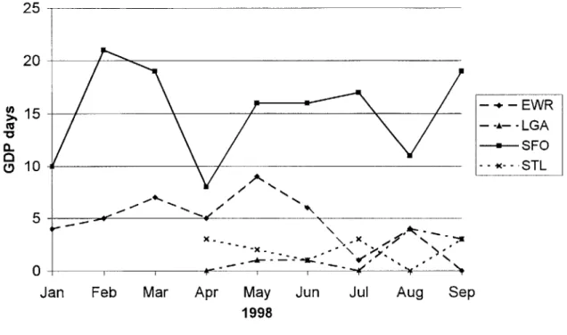
Table 2-1 summarizes the number of GDP-E programs that were run at the four prototype operations airports during the first nine months of 1998. The table shows the number of days with GDPs (days), as well as the actual number of programs (progs), since a given day may have more than one program associated with it. An

into effect for LGA and STL until the month of

entry of '-' indicates that GDP-E did not go April. The same data is plotted in Figure 2-1.

Month EWR EWR LGA LGA SFO SFO STL STL

Days Progs Days Progs Days Progs Days Progs

Jan

Table 2-1: Ground delay programs

SFO stands out clearly in the overall number of programs run, with an average of 10.6 GDP days per month and 15.2 programs per month. Another way to look at this is that SFO had a GDP every 2.8 days. The other three airports being analyzed have a much lower overall incidence of GDP programs.

25 20

15

Jan Feb Mar Apr May Jun Jul Aug Sep

1998

Figure 2-1: Ground delay programs

2.2.3 SFO hourly distribuion of ground delay

programs

Additional insight into the incidence of GDP programs can be obtained by examining the frequency with which GDPs were in effect, as a function of time of the day. SFO was used as the base for this analysis due to its large volume of programs actually run. Figure 5 shows, for each hour, the number of days that SFO had an active-GDP or a cancelled-GDP.

90

80

_--

_{Active GDP}

-Cancelled

60

50

040--30

20

10

0-6

7

8

9 10 11 12 13 14 15 16 17 18 19 20 21 22 23 24

Figure 2-2: SFO incidences of GDPs, by hour

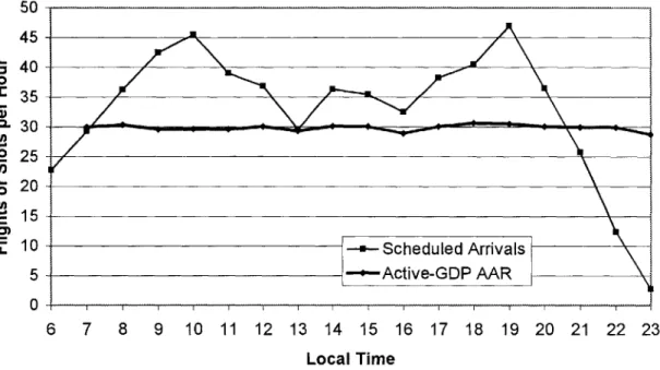
Since GDPs are instituted in response to anticipated shortfalls in capacity, GDPs have a close affinity to the scheduled demand profile. Table 2-2 and Figure 2-3 explores this further. In the table, sched is the average scheduled number of arrivals per hour and AAR is the average AAR.

Hour 7 8 9 10 11 12 13 14 15 16 17 18 19 20 21 22 23 Sched 29.3 36.2 42.5 45.5 39.0 36.8 29.6 36.3 35.5 32.5 38.2 40.5 46.9 36.4 25.7 12.4 2.7 AAR 30.0 30.3 29.6 29.6 29.6 30.1 29.3 30.2 30.1 28.9 30.1 30.7 30.5 30.1 29.9 29.9 28.8 Table 2-2: SFO average scheduled arrivals and active-GDP AARs

Table 2-2 and Figure 2-3 indicate a uniformly higher demand than the average AAR in the hours between 8:00 and 21:00. The morning demand peaks in the hour between 10:00 and 11:00, and the afternoon peak is between 19:00 and 20:00. These peaks are much more pronounced that the ones found in Figure 2-2, where the incidences of GDPs were plotted. The data shows that the airport activity level during a GDP remains almost constant throughout the day, which is due to the near-uniform use of an SFO AAR of 30. Note that the average active-GDP AAR remains at this level beyond 21:00. This can be attributed to accommodating flights that have been delayed by the GDP programs.

50 45 - S40-0 Z 35 C- 30 - 25 0 20 U) S15-S10- - Scheduled Arrivals L.5 -+-Active-GDP AAR 0 -- --- -- ,--- ,- , , I I , I ,---6 7 8 9 10 11 12 13 14 15 16 17 18 19 20 21 22 23 Local Time

Figure 2-3: SFO average scheduled arrivals and active-GDP AARs, by hour

Figure 2-2 shows that the cancelled-GDPs also has a bimodal distribution, albeit shifted 3 to 5 hours later in the day from the active-GDP peaks. They thus follow the morning and evening post-peak arrival times as shown in when the arrival rates start to drop and capacity is less constrained.

2.2.4 Seasonal variation ofground delay programs

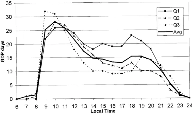
The seasonal variation can be explored by analyzing the data over the available quarters. Figure 2-4 shows the seasonal variation in the incidence of the SFO GDPs, and Figure 2-5 shows the similar variation of the EWR GDPs.

35

25

>%20

a-15

10

*

5

0

6

7

8

9 10 11 12 13 14 15 16 17 18 19 20 21 22 23 24

Local Time

Figure 2-4: SFO quarterly incidences of GDPs, by hour

16

14

12

10

8

6

4

-2

0

6

7

8

9 10 11 12 13 14 15 16 17 18 19 20 21 22 23 24

The seasonal variability of SFO GDP incidences seems quite low. As can be seen from Figure 2-4, each quarter exhibits the characteristic shape of the average, with some variations. The biggest difference is found in the early afternoon number, where there has been a substantial decrease of almost 50% from quarter 1 to quarter 3. What this decrease is due to is impossible to say based on the data at hand, but possible candidates are seasonal weather variations, better execution of the GDPs, the effects of compressions, or a combination of all of these and others.

Figure 2-5 shows that the EWR incidence of GDPs is quite different from the one at SFO. First, the averages are much lower overall. At EWR, the quarterly peak of 14 GDP days is reached in the 2"d quarter in the hour between 17:00 and 18:00. At SFO, the quarterly peak of 32 GDP days is reached in the 3rd quarter between 9:00 and 10:00. A similar pattern holds for the statistics of the full nine months studied. The average GDP days per quarter rises to a peak of 9 GDP days per quarter at EWR, and 28 GDP days per quarter at SFO.

Second, there is a much larger variation from quarter to quarter found at EWR. SFO basically maintains the same pattern for all three quarters, with some variations found especially during the secondary peak in the later afternoon hours. EWR on the other hand sees a dramatic lowering in the third quarter. This results from just three GDP days in this quarter.

Third, there is a fundamental difference in the shape of the two curves. SFO has a pronounced and sharp peak in the morning, probably as a result of the morning fog being a very consistent feature at this airport, followed by a substantial drop to a level that is then sustained from the noon hour through about 20:00 in the evening. EWR has a much smoother shape. GDPs typically do not take effect until after 12:00, but then last a bit longer, extending through to 23:00.

2.3 Substitution and Compression Analysis 2.3.1 Methodology

The effects of substitutions and compressions under CDM are analyzed by initially determining the effect on individual flights, and then aggregating the results as appropriate.

The AADL files contain information about each flight's change in estimated arrival time. Each of these changes are classified and aggregated into one of four categories.

FAA arrival slot allocation delays: Any change made during a 20 minute window2_{, starting at the}

time of a GDP initiation, revision, extension or revision/extension, is deemed to belong to the FAA arrival slot allocation delay category. The incremental delay (calculated as the difference between the previous and current setting of the ETA field) is added to cumulative FAA arival slot allocation delay field for that flight.

Airline substitution delays: If a flight moves into a controlled time of arrival (CTA) slot previously occupied by another flight from the same airline, and this happens outside the 20 minute window timeframe of any FAA-initiated GDP program action, then that change is deemed to belong to the airline substitution category. The incremental delay (calculated as the difference between the previous and current setting of the ETA field) is added to the cumulative airline substitution delay field for that flight. An airline and all of its subsidiaries are looked upon as a single entity when deciding which slot swaps belong in this category.

Compression delays: Any change made during a 20 minute window, starting at the time of a GDP compression, is deemed to belong to the compression category. The incremental delay (calculated as the difference between the previous and current setting of the ETA field) is added to the cumulative compression delay field for that flight. These delays are in actuality negative numbers, representing a time saving.

Other delays: This is a catch-all category established to collect those changes that cannot be ascribed to any of the above three reasons. It is typically used infrequently, i.e., typically less than 3 times per day, and the changes it makes are generally the result of some errors in the

2 The 20 minute window used during the determination of the delays is a historical artifact. Initially the GDP program fles did not contain information about exactly when a given change took effect in the system (and hence in the AADL files), only when they were applied. There typically was a 10 minute gap between the time of applying the changes and the time when they took effect, but this gap could and did vary somewhat. Employing the 20 minute window ensured that the changes got attributed to the correct cause of the change.

This situation has already been corrected as far as the availability of the data is concemed. Any analysis of data after 7/22 can dispense with the time window and use the exact time of the changes taking effect, since this data is now contained in the AADL files. Before this can be put into use, though, some computer program changes will be needed.

underlying data. The incremental delay (calculated as the difference between the previous and current setting of the ETA field) is added to the cumulative other delay field for that flight.

These calculations take place during the data extraction phase, and only the net result per flight for each of the four categories is brought forward and stored into the database.

2.3.2 Satings

The benefits of substitutions and compressions were measured by calculating the savings directly attributable to each. Table 2-3 summarizes the results of the first 9 months of GDP-E prototype operations.

Airport EWR LGA SFO STL Overall

All flights 57,190 122,540 145,278 172,740 597,748

GDP flights 9,241 1,571 28,713 3,263 42,788

GDP flights % 5.90% 1.30% 19.80% 1.90% 7.2%

Ground delay allocated (hrs) 14,681 1,692 59,841 6,936 83,151

Substitution savings (hrs) 1,533 176 5,341 670 7,720

Compression savings (hrs) 934 57 3,108 542 4,641

Net delay (hrs) 12,214 1,459 51,392 5,724 70,789

Substitution savings % 10.4% 10.4% 8.9% 9.7% 9.3%

Compression savings % 6.4% 3.4% 5.2% 7.8% 5.6%

Subst savings per Flight (min) 10.0 6.7 11.2 12.3 10.8

Comp savings per Flight (min) 6.1 2.2 6.5 10.0 6.5

Table 2-3: Airline substitution and GDP compression summary results

In this table, A//flights is the total count of flights that arrived at the airport. GDPfights is the subset of flights that at one point or another had a GDP arrival slot allocated, and GDPfights % is the percentage of flights that were affected by a GDP.

Ground delay allocated is the net sum of all delays allocated by the GDPs. Each flight might be subject to multiple delay changes. The initial delay assigned will always be a positive delay, but subsequent changes may be either positive or negative, reflecting worsening or improving conditions. Substitution savings are the savings that are recouped by the airlines substituting one flight for another (and canceling some flights), and compression savings are the savings from running the GDP compression algorithm. The net dela) is the final delay after airline and compression savings have been applied.

Substitution savngs % measures how effective substitution is in reducing the delay allocated by the GDPs, and compression savngs % similarly measures the effect of compressions. Subst savings perpght is calculated by averaging the substitution savings over every GDP flight, and cop

savingsperpght similarly measures the savings due to compression per GDP flight.

It is evident that substitutions and compressions both contribute substantial benefits to the system. The average compression savings is 5.6%, with a low of 3.4% at LGA and a high at 7.8% at STL. SFO is at 5.2% and EWR at 6.4%. Similarly, the average substitution savings are 9.3%, with a high of 10.4% in both EWR and LGA, and a low of 8.9% in SFO. It is also clear that GDPs affect SFO far more extensively than any of the other three airports studied. This is primarily due to the local weather conditions and overall arrival capacity at SFO.

2.3.3 Monthly results

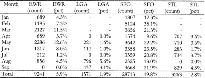
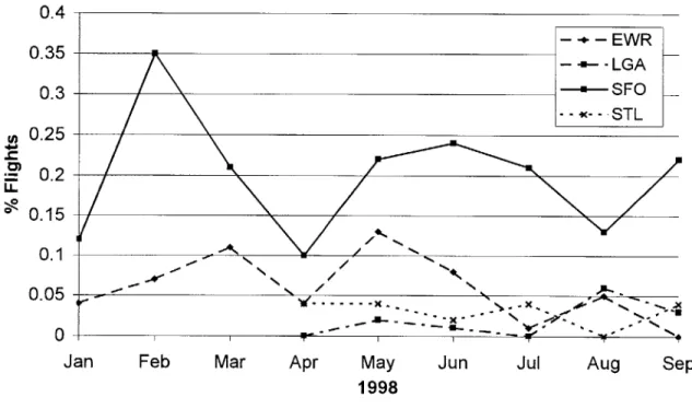
The results can be analyzed in more detail by examining the data on a monthly basis. This is done in Table 2-4 and Figure 2-6. The table and the figure show the number of GDP flights for each airport (coun), as well as the monthly percentage of flights affected by GDPs (pct).

Month EWR EWR LGA LGA SFO SFO STL STL

(count) (pct) (count) (pct) (count) (pct) (count) (pct)

Jan

Jun

Jul

Table 2-4: Flown flights that were at some point affected by GDP

SFO again stands out clearly as being much more heavily subjected to GDP delays than the other three airports. February is an especially heavily impacted month, maybe due to the effects of El Nifio.

0.4

_0.35--

LA--0.3

-

--Jan

Feb

Mar

Apr

May

Jun

Jul

Aug

Sep

1998

Figure 2-6: Flown flights affected at some point by GDP

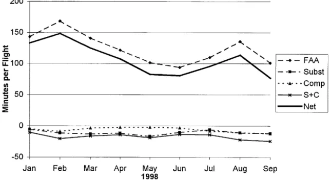
2.3.4 SFO monthly delay classification

The net GDP delays can be determined by looking at the core components affecting these delays: first, the initial FAA arrival slot allocation delay, along with any subsequent revisions; second, savings associated with airline substitutions; and third, savings that come about as a result of using the compression algorithm.

Each of these are measured on a per-month basis in Table 2-5. In this table, FAA tallies the FAA arrival slot allocation delays, subst is the savings resulting from airline substitutions., and comp is the savings resulting from compression. S+C is the combined savings from substitution and compression, and net is the net sum of all these measures. S+C% shows the monthly savings as a percentage of total delay handed out, and S % and C % shows the percentage savings resulting from substitution and compression respectively.

Month FAA Subst Comp S+C Net S+C % S% C %

Jan

Feb 168.4 -11.5 -8.6 -20.1 148.3 12.0% 6.8% 5.1%

Mar 140.8 -12.8 -3.3 -16.1 124.7 11.4% 9.1% 2.4%

Apr 121.7 -11.8 -2.4 -14.1 107.6 11.6% 9.7% 1.9%

Month FAA Subst Comp S+C Net S+C % S% C % Jun 93.9 -10.1 -3.3 -13.4 80.5 14.3% 10.8% 3.5% Jul 109.7 -6.2 -8.0 -14.2 95.6 12.9% 5.6% 7.3% Aug 135.8 -11.1 -10.9 -22.1 113.7 16.2% 8.2% 8.0% Sep ...100.9 -11.8 -12.4 -24.2 -76.7 24.0% 11.7% 12.3%/ Average 125.0 -11.2 -6.5 -17.7 107.4 14.1% 8.9% 5.2%

Table 2-5: SFO average delay and delay savings per GDP flight, by month

200 150 0> U 100 50 CI !9 FAA -- - Subst --- Comp -- S+C Net

0

Jan Feb Mar Apr May Jun

1998

Jul Aug Sep

Figure 2-7: SFO substitution and compression savings per GDP flight, by month

The data suggests a possible improving trend in the delays, dropping from a net delay of 148.3 minutes per flight in February to a low of 76.7 minutes in September. There are, however, substantial month-to-month variations within this time-period. The drop in average may be due to seasonal factors, but this will become clearer only when data for several years become available. February clearly was a difficult month. Not only were there more flights delayed during that month (see Table 2-4), but each delayed flight was also delayed for a longer period of time. This may have been due to the effects of El Nino.

The delay savings resulting from the combination of airline substitutions and GDP compression are also quite noticeable, especially in the figure. Averaged over all GDP flights to arrive in SFO, the delay is reduced by 17.7 minutes per flight, from 125.0 minutes on

average to 107.4 minutes or average. This is equivalent to a savings of 14.1%, of which 5.2% resulted from compression. The composition of the combined savings changed starting in July. Until then, airline substitutions clearly accounted for most of the savings, but from July on the savings from substitutions and compressions are almost identical. One possible explanation is that it reflects a maturing of the compression process. Another possibility is that the airlines are becoming more comfortable with the compression process and the results that it is producing, and are showing this by cutting back on the number of substitutions they are initiating. It does not, however, appear to be a consequence of fewer cancellations. Table 2-24: Average daily cancellationsfor GDP and non-GDP days shows that the number of cancellations per GDP day has remained fairly constant. This is important, since the benefit from a substitution, as far as a time saving is concerned, only arises when a flight gets cancelled and another flight assigned by the GDP to a later arrival slot can be moved up to take the former's CTA in the stream of arrivals. (An airline may obtain benefits from swapping two active flights with one another, but these benefits do not include any aggregate time saving, and so do not affect the results being measured here).

Note that the savings from airline substitutions and from GDP compression both increase over the nine month period studied. This is an indication that the CDM benefits are not derived solely from the introduction of compression, but that a portion of the airline substitution savings also needs to be attributed to CDM. However, it is also reasonable to assume that some of the benefits derived from GDP compression could have been obtained by additional airline substitutions in the absence of GDP compression. Since data has not been available for the period prior to the startup of GDP-E, it is not possible to state what a lower bound on the benefits of introducing CDM have been as SFO. The combined savings resulting from substitution and compression savings form an upper bound of 14.1% on the derived benefits. The 5.2% resulting from compression is an indication of this lower bound, but further analysis and data is required to determine this with greater certainty.

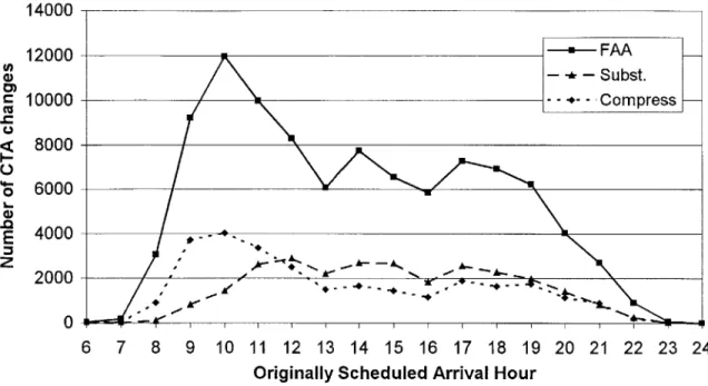
2.3.5 SFO hourly results

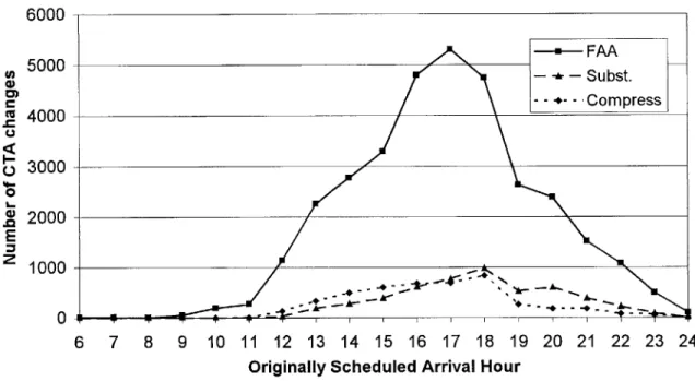
Analyzing the same data on an hourly basis yields further insight into the use of the SFO GDPs. The two following figures illustrate this. Figure 2-8 depicts the number of changes made to the CTA as a function of the time of day of the originally scheduled time of arrival.

U) 0 E

z

10000

Figure 2-8: SFO number of CTA changes, by hour

E

E

Cu

Originally Scheduled Arrival Hour

Figure 2-9: SFO ground delay, by hour

FAA Subst.

eCompress-,-- +--

Figure 2-8 shows the large number of delay assignments made to the morning-hour flights into SFO, caused by the large number of scheduled flights during these hours and the prevalence of GDP programs. Two smaller secondary peaks are also in evidence later in the day, probably for the same reason.

It is also evident from this figure that compression picks up earlier than substitutions. The absolute number of compression-related changes is four times as high as the number of airline substitutions for arrivals between 9:00 and 10:00. However, from 11:00 on the number of changes attributable to these two factors are quite close to one another.

Figure 2-9 shows the ground delay allocated by the FAA arrival slot allocations, and the portion of this delay recovered by airline substitutions and compressions, again as a function of originally scheduled time of arrival. This shows the impact that the changes have on the total arrival delay. First, two peaks stand out, matching the time period of the morning and afternoon peak arrival demand (see also Figure 2-3: SFO average scheduled arrivals and active-GDP AARs, bv hour). Second, the effects of both substitution and compression improve over the time of day, with the combined effect being twice as large on the afternoon peak as it is on the morning peak. Third, airline substitutions play a larger role than compression in reducing delays. However, as was shown earlier in the monthly analysis for SFO, savings attributable to airline substitutions and to compressions were almost equal in the last three month of the study period. The larger airline substitution savings shown in Figure 2-9 probably reflect in part the initial prototype operation of compression.

2.3.6 EfWR hourly results

A similar analysis follows for EWR. Figure 2-10 shows the number of changes in the allocated delay, the airline substitutions and the compressions. Figure 2-11 shows the effect that these changes have on the various GDP delay measures.

U) 0) E 0

z

-

Figure 2-10: EWR number of CTA changes, by hour

CU

.0

350,000

300,000

250,000

200,000

150,000

100,000

50,000

0

-50,000

-100,000

6

7 8 9 10 11 12 13 14 15 16 17 18 19 20 21 22 23 24

Originally Scheduled Arrival Hour

Figure 2-10 shows the situation at EWR to be considerably different from the one found at SFO. There are a lot fewer changes overall. The number of changes made in response to the FAA arrival slot allocations are also a lot fewer, both for airline substitutions and especially for GDP compressions. The impact of compression at EWR is much smaller than what was seen at SFO. This is also confirmed by the data in Figure 2-11, which depicts the delays. The delay savings attributable to compression after 20:00 are very small when compared to both the arrival slot allocation delay and even the substitution savings.

2.4 Arrival Slot Utilization

Compression and airline substitutions provide one avenue for improving the overall effectiveness of the system. They do so in two ways. First, they lower the average delay imposed on flights. Second, they may decrease the variability of the inter-arrival times. The use of compression increases the likelihood that a steady stream of flights arrive at the destination airport. This could ultimately lead to a lowering of the Managed Arrival Reservoir (MAR), which in turn should result in a lowered airborne holding.

A second avenue for improving the overall system is to ensure that the available arrival capacity at the GDP airport is utilized to its fullest. Measuring GDP arrival slot utilization helps answer this latter question, and is the subject of this section.

2.4.1 Methodology

There are two basic steps in the analysis. First, we determine the supply of and demand for capacity for every hour. Second, we aggregate the hourly results according to needs of the analysis.

Actual hourly demand is determined by counting how many flights actually arrive in a given hour at a given airport. In addition to this, scheduled demand is also needed, for reasons that will become clear shortly. Both types of information are readily available from the database.

Hourly capacity is provided as part of the GDP program parameters. Every time a GDP is initiated or revised, it is accompanied by a specification of the AARs and GA factors for the hours affected by the GDP. As such, capacity information is readily available for the GDP hours. Unfortunately, there is no similar source of capacity information available for the

non-GDP hours.3 One impact this has on the analysis possibilities is to make it difficult to

judge

how quickly operations return to normal following the cancellation of a GDP program, since the arrival capacity and hence the upper bound on the arrivals is unknown.

To fully explain capacity utilization, two additional aspects need to be addressed. The first issue deals with the situation when multiple AARs have been successively specified for the same hour. Currently, only the last value specified is used, on the assumption that it contains the latest and therefore best estimate of the actual conditions for that hour. However, any earlier settings of an AAR will have governed the arrival slot allocation for some amount of time. As such, it is entirely possible that there is a relationship between when an AAR can be changed, and how quickly these changes can have a real effect on the system. This remains an open research topic to be investigated.

The second capacity aspect to be covered concerns the issue of what to do when demand is too low to fully utilize a given capacity. This is either caused by not allocating enough flights for the given hour, or if simply there are not enough scheduled and delayed flights to fill the available capacity for that hour. To deal with this an adjusted capacity AAR' is used in place of the stated AAR capacity. The adjusted capacity is defined as: (1) AAR' = AAR, when scheduled arrivals exceed or equal the available capacity, and (2) AAR' = actual arrivals, when scheduled arrivals is less than the available AAR capacity. The primary benefit of using AAR' in place of AAR is that it avoids denoting unused capacity as under-utilized.

GDPs are typically neither instituted nor cancelled on even-hour boundaries. This raises the issue of how to classify the hours that contain such a change. The approach adopted here is to treat these hours as active-GDP hours. This may register as a slight overuse of the restricted capacity, since the period prior to or following an active-GDP typically will have a larger capacity, but it errs on the side of caution. However, the overall effect of this is judged to be minimal.

Table 2-6 illustrates these concepts. The table contains a subset of the demand and capacity information for SFO on 9/30/1998, when a GDP was in effect.

3 _{This is one of the gaps in the data needed for the analysis. Hopefully this can be remedied in the future, possibly by inclusion} of airport configuration information in the AADL fles that already provide the bulk of the core analysis data.

Dest Hour GDPs Sched Flown Cnx Land AAR AAR' Unused Pct

SFO 20 1 48 36 12 31 30 30 -1 -3%

SFO 21 1 36 25 11 32 30 30 -2 -6%

SFO 22 1 24 18 6 28 30 28 0 0%

Table 2-6: Adjusted arrival capacity (AAR') example

The hour starting at 20:00 (hou) covers 1 hour of GDP (GDPs). It originally had 48 flights scheduled to arrive at that hour (sched), out of which 36 flights were flown (flown) and 12 were cancelled (cnx). 31 flights actually arrived during this hour (land). The data provide no information about when these particular 31 flights originally were scheduled to land, but it is unlikely that they all came from the original pool of 48 scheduled flights for that hour. The stated AAR capacity was 30 flights per hour (AAR), which is the last set value for the AAR capacity for this hour. The adjusted AAR capacity for this hour is also 30 (AAR'). The number of unused slots are -1 (unused), calculated as AAR' - land. Finally, the slot capacity under-utilization is -3% (pct), calculated as unused/AAR. In this instance, the last two columns show that one more flight landed than was planned for.

The hour starting at 22:00 shows the effect of the adjusted capacity calculation. 24 flights were originally scheduled to arrive at this hour, which is less than the available capacity of 30. As a consequence, the adjusted capacity is set to 28, the number of flights that actually arrived at this hour.

2.4.2 SFO hourly arrival slot utilization

The hourly arrival slot utilization at SFO has been analyzed to answer the question of whether or not the available capacity is being used to its fullest extent. Table 2-7 summarizes this analysis. In this table, LocalHour is the local hour of day, i.e., in PST or PDT. Active-GDP days counts the number of days when a GDP was active for that particular hour, and cancelled-GDP days similarly counts the number of days when a GDP had initially been planned for that hour, but was subsequently cancelled. Unused active slots is the sum total of active-GDP slots that went unused in that hour, and similarly for the unused cancelled slots. In the latter case this number is going to be negative, representing an overuse which is to be expected when the capacity constraints are lifted. Net unused slots is the difference between the previous two columns. Finally, the last three columns, unused active slots/dajv, unused cancelled slots/dy, and net unused slots/ dy show a daily average for each slot measurement.