To cite this version
Ayter, Julie and Desclaux, Cecile and Chifu,
Adrian-Gabriel and Déjean, Sébastien and Mothe, Josiane Performance Analysis of
Information Retrieval Systems. (2014) In: Spanish Conference on
Information Retrieval (), 19 June 2014 - 20 June 2014 (Coruna, Spain)
OATAO is an open access repository that collects the work of Toulouse researchers
and makes it freely available over the web where possible.
This is an author-deposited version published in:
http://oatao.univ-toulouse.fr
/
Eprints ID : 13047
Any correspondance concerning this service should be sent to the repository
administrator:
[email protected]
Julie Ayter1, Cecile Desclaux1, Adrian-Gabriel Chifu2, Sebastien Déjean3, and Josiane Mothe2,4
1
Institut National des Sciences Appliquées de Toulouse (France) 2
IRIT UMR5505, CNRS, Université de Toulouse, Toulouse (France) [email protected] 3
Institut de Mathématiques de Toulouse (France) [email protected] 4
Ecole Supérieure du Professorat et de l’Education (France) [email protected]
Abstract. It has been shown that there is not a best information retrieval system con-figuration which would work for any query, but rather that performance can vary from one query to another. It would be interesting if a meta-system could decide which system should process a new query by learning from the context of previously submitted queries. This paper reports a deep analysis considering more than 80,000 search engine configura-tions applied to 100 queries and the corresponding performance. The goal of the analysis is to identify which search engine configuration responds best to a certain type of query. We considered two approaches to define query types: one is based on query clustering ac-cording to the query performance (their difficulty), while the other approach uses various query features (including query difficulty predictors) to cluster queries. We identified two parameters that should be optimized first. An important outcome is that we could not obtain strong conclusive results; considering the large number of systems and methods we used, this result could lead to the conclusion that current query features does not fit the optimizing problem.
Keywords: Information Retrieval, Classification, Query difficulty, Optimization, Random Forest, Adaptive Information Retrieval
1
Introduction
Information Retrieval (IR) is a very active research area that aims at proposing and evaluat-ing indexevaluat-ing, matchevaluat-ing and rankevaluat-ing methods to retrieve relevant documents accordevaluat-ing to users’ queries. Many models have been defined in the literature, most of them having various param-eters. To evaluate a model, the IR community relies on international benchmark collections, such as the ones from the Text REtrieval Conference (TREC)5
, composed of sets of documents, topics, relevance judgments and performance measures. It has been shown that there is an im-portant variability in terms of queries and systems for these collections. System or search engine variability refers to the fact that there is not a best system. A single configuration of a search engine that would treat any query as an oracle does not exist; rather, specific search engines are better for specific queries. By the way, system variability has not been deeply studied. Are systems sensitive to query difficulty? Are they sensitive to other query characteristics? If it is the case, some systems would be specialized in some types of queries. For example, ambiguous queries would need a system that first disambiguates the query terms, particular queries would be improved if first expanded, etc.
Having in mind the system variability, our goal is to identify which search engine (or con-figuration) would respond best for a particular type of query. If we were able to characterize query types and learn the best system to each query type, then, for a newly submitted query,
5
we would be able to decide which system should process it. This requires to thoroughly analyze systems, queries and obtained results, in order to find whether some system parameters are more influential on results and whether this influence is query dependent.
This paper reports a deep analysis considering more than 80,000 search engine configurations applied to 100 queries and the corresponding system performance. The data set is described in Section 3. Section 4 reports the analysis of the system parameters according to query types. Defining query types is not obvious. We considered two approaches: the first one is based on clustering queries according to the query difficulty; the second approach uses various query features to cluster queries. Section 5 concludes the paper.
2
Related Work
Statistical analysis of search results. Some studies in the literature have been conducted using statistical analysis methods to observe search results over sets of queries. In [1] the author analyzed TREC results; their data set consisted in the average precision values (see Section 3) for systems, on a per query basis. Various data analysis methods were used to identify the existence of different patterns. However, the authors stated the results are inconclusive. The same type of data matrix was used in [2], where the authors employed hierarchical classifications and factor analysis to visualize correlations between systems and queries. Mizzaro and Robertson [3] aimed at distinguishing good systems from bad systems by defining a minimal subset of queries obtained from data set analysis. The authors concluded that "easy" queries perform this task best. Dinçer [4] compared performances of various search strategies through the means of Principal Component Analysis. Compaoré et al. [5] employed, as we do, indexing parameters and search models to determine which parameters significantly affect search engine performance. However, the number of parameters they used was significantly lower.
System variability and query difficulty.System variability is a major issue when choos-ing the most fitted system for a certain query. Harman and Buckley [6],[7] underlined that understanding variability in results (system A working well on topic 1 but poorly on topic 2 and system B behaving in an opposite manner) is difficult because it is due to three types of factors: topic statement, relationship of the topic to the documents and system features. Query difficulty is closely linked to system variability. Some features have been shown to predict query difficulty; these predictors cover various aspects of the three previous factors: term ambiguity (the number of WordNet senses for query terms [8]), term discrimination (IDF [9]), document list homogeneity (NQC [10]), and result lists divergence (QF [11]).
Clustering queries. In this paper, we use query difficulty predictors as features for query clustering. We then learn a model to associate a query cluster to the relevant system; in this way any new query that can be associated with an existing cluster can be processed by the corresponding system. In [12] query features were also used to cluster TREC topics. The best term-weighting schema in terms of precision/recall measures was then associated with each topic cluster. Different term weighting schemas were applied depending on query characteristics. On TREC Robust benchmark, this method improved results on poorly performing queries. Kurland [13] considered query-specific clusters for re-ranking the retrieved documents. Clustering queries has also been studied in the web context, based on query logs [14]. Bigot et al. [15] showed how to group queries by their difficulty, using TREC submission results for training. A new query for the system, according to its type, was then assigned to the right search engine. Mothe and Tanguy [16] also showed that queries can be clustered according to their linguistic features and that these features are correlated with system performances. In addition, combining various predictors for a better correlation with query performance [17],[18] also suggested that query difficulty predictors values could represent features to differentiate query types.
3
Data set presentation and descriptive analysis
The data we analyze in this paper has been built by using various search engine components and parameters on TREC adhoc collections. To do so, we used the Terrier6
platform.
TREC provides various topics corresponding to users’ needs (having three parts: title, de-scriptive and narrative). Queries for retrieval could be constructed from these topics. TREC also provides the documents for the search and relevance judgments to evaluate the retrieval results; several performance measures can be computed. On the other hand, the Terrier environment provides several modules and parameters for indexing, retrieval and query expansion models.
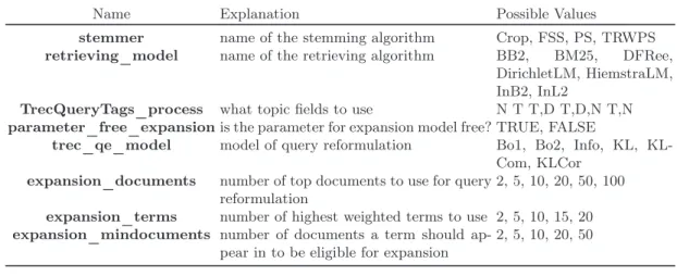
The initial data set was built using about 80,000 different combinations of term weights, retrieval algorithms and parameters applied on 100 queries. The redundant parameters were filtered out; 8 parameters were kept (1 for indexing, 2 for retrieval and 5 for query expansion) for which different values were chosen (see Table 1). Subsequently, the results were evaluated using the Average Precision (AP) performance measure. AP is extensively used in IR to compare systems effectiveness [19]. Indeed, the average of APs across all the queries is the Mean Average Precision (MAP) and represents a global performance measure for a system. Finally, the analyzed data set was made of 8,159,800 rows and 10 columns (8 parameters, 1 query, 1 for the AP).
Table 1. The considered parameters for the analysis
Name Explanation Possible Values
stemmer name of the stemming algorithm Crop, FSS, PS, TRWPS retrieving_model name of the retrieving algorithm BB2, BM25, DFRee,
DirichletLM, HiemstraLM, InB2, InL2
TrecQueryTags_process what topic fields to use N T T,D T,D,N T,N parameter_free_expansion is the parameter for expansion model free? TRUE, FALSE
trec_qe_model model of query reformulation Bo1, Bo2, Info, KL, KL-Com, KLCor
expansion_documents number of top documents to use for query reformulation
2, 5, 10, 20, 50, 100 expansion_terms number of highest weighted terms to use 2, 5, 10, 15, 20 expansion_mindocuments number of documents a term should
ap-pear in to be eligible for expansion
2, 5, 10, 20, 50
3.1 Descriptive statistics
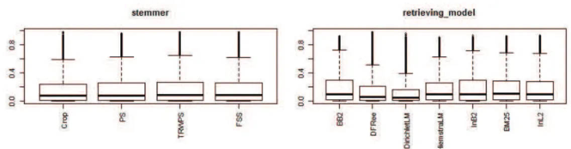
First of all, we wanted to see if some parameters were obviously better than others, as far as the MAP is concerned. Figure 1 shows the boxplots of the MAP for each value taken by each search parameter. The boxplots are very similar from one parameter value to another. For example, the median and the first and third quartiles of the MAP are almost identical for the four stemming algorithms that were tested.
Regarding the term weighting methods, there are a few differences: boxes of the DFRee and DirichletLMmodels are a little thinner and lower than boxes of the other algorithms. It means that both their median and their variability are smaller than those of other algorithms. However, this difference is not strong enough to conclude that these two algorithms are worse than the rest.
6
Fig. 1. Boxplots of the MAP for the first two parameters
We can also see that most of the good MAP values are outliers, which means that few systems and queries give good results (less than 10% of the data with a specific value of a parameter). Consequently, it may be difficult to efficiently predict good MAP results. Finally, we can notice that the first quartile of the boxplots is very close to 0 and most of the MAP values are smaller than 0.4, which means there are many systems that give bad results and there might also be a lot of rows for which the MAP is null.
3.2 Poorly performing queries and systems
There is a large number of low MAP values (as seen in Section 3.1). If there are much more bad results than good ones, a predicting model will tend to predict bad results better than good results. For this reason, they should be removed from the dataset in order to be able to focus on good results. There were 437, 672 rows with a null MAP and almost 70, 000 systems have at least one query with a null MAP, thus we could not remove all of them from the data set without losing a lot of information. Another lead was to check whether any particular queries yielded worse MAP values than others. We underline that queries 442 and 432 are responsible for many more null MAP values than other queries representing 11.9% and 11% of the null data, meaning that these queries are much harder than the others.
We finally remove the parameter combinations that yielded really bad results, no matter what the query was. Doing so, by removing about 2.5% of the data, we removed more than 30% of the MAP values that were equal to 0, while ensuring that the distribution of the results in the new data set was similar to the original one.
4
System parameter tuning based on query performance
There is not a single best system for all the queries thus defining a model that could work for unseen queries implies to learn somehow from query characteristics. For this reason, we define clusters of queries for which we aim to associate a system with, making the hypothesis the most efficient systems would be different depending on the query cluster. Defining query clusters is not obvious. Two complementary approaches have been used to define query clusters. The first one is based on query difficulty. In the second approach, we cluster queries according to query characteristics such as their length, their IDF, query difficulty predictors, etc.
4.1 Clustering queries according to their difficulty
We cluster the queries evenly proportioned, according to their difficulty as measured by the MAP: easy, medium and hard queries.
Analysis of variance The first question we wanted to answer was if all parameters have a significant effect on the MAP results. It would not directly help finding the best system, but it could reduce the number of parameters to optimize. Moreover, some parameters could have an influence on easy queries and none on hard ones, for example.
In order to study this significance, we performed analysis of variance (ANOVA)[20] tests on the three query difficulty levels. Due to the size of the data set, we could not test all queries in a complexity level, but instead we randomly selected two queries for each cluster.
In a first model, we considered there was only one effect: the parameter we wished to study: APij = µ + parami+ ǫij, where ǫij ∼ N (0, σ2)
parami is the effect of the i th
value of the parameter on the MAP measure. This was done for each of the eight parameters.
In a second model, we considered all effects at the same time with no interaction: APi= µ + param1k1(i)+ ... + param8k8(i)+ ǫi, where ǫi∼ N (0, σ
2)
kj(i) is the value taken by the jth parameter for the ith system.
These two models were only applied to six randomly chosen queries with the following con-clusion: all parameters seem to be significant, no matter what the query difficulty is, except for the free expansion parameter (one non significant p-value). As a result, all the parameters should be kept in the following analysis.
Classification and regression trees We noticed that all parameters had an influence on MAP values, but ANOVA tests do not tell what values to give for these parameters toward optimizing the results. Indeed, if we could find a model that predicts well the data, we might be able to use it in order to optimize the parameters and to get the best MAP as possible for any query.
The first statistical approach we used to model the data was Classification And Regression Trees (CART) [21]. An advantage of this method is that, besides predicting results, we can see which are the best discriminating variables by plotting the trees.
Here, we are not interested in knowing exactly what the MAP value will be for one combi-nation of parameters, we would rather like to know how good this value will be. Therefore, we need to define what a good or bad result is. In order to do so, we looked at the first and third quartiles of the MAP for each query group and decided that the results would be good when they were greater than the third quartile, bad when they were lower than the first quartile and average otherwise. Trees were computed for all systems and all queries of each complexity level. Pruning was performed by setting a threshold on a complexity parameter in order to provide more interpretable trees.
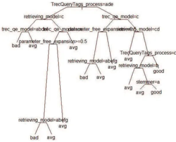
Hard queries. With regard to hard queries (Figure 2), there are two "good" predictions and they occur when using the fields (TrecQueryTags_process) TITLE or TITLE, DESC, the reformulation algorithms (trec_qe_model) Bo1, Bo2, KL, KLCom or KLCor and the retrieving model algorithms either BB2, DFRee, InB2, BM25 or InL2. Also the stemming algorithm has an importance in one of the predictions.
Medium queries. The predictions are very similar to hard queries, except for the stemmer algoritm which is not involved for "good" predictions.
Easy queries. The query reformulation model (trec_qe_model parameter) best discriminates the MAP results, it separates the systems with the Info algorithm from those with other algo-rithms. However, no combination of parameters gives "good" results, and we only got "bad" and "average" decisions. This is not very satisfying because it means that this method does not allow us to predict the best results and, therefore, to know what parameter values to use. There are a
few "bad" results, so at least we know which parameter values to avoid. For example, when the Info algorithm is used and the parameter for expansion model is free, it is very likely that results will be "bad".
Fig. 2. Classification tree for hard queries
To conclude, we noted that results were not always satisfactory as they could not always predict "good" MAP values. Nevertheless, it is more interesting to know which parameters to be careful about with hard queries than with easy ones. Indeed, for easy queries, results are supposed to be quite good and parameter values do not have a big influence, as opposed to hard queries.
Notice that CART tends to be quite unstable. To confirm the previous results, we used random forests [22]; the drawback of random forest is that the results are more difficult to interpret. Random Forests The algorithm randomly chooses a given number of variables (among all the variables of the data) for every split of classification trees. Many trees are computed in this manner and results are averaged in order to obtain an importance measure for each variable, based on the changes its presence or absence caused. We used this method on each of the three query difficulty clusters and we optimized the number of variables to select. For computational reasons we applied random forests to 10,000 randomly chosen training rows.
We used cross-validation and an accuracy measure to fix the number of variables to select. The accuracy was the greatest when there were four parameters in the trees, for every complexity level. The accuracy decreases with the growth of the number of variables.
We plotted the parameter importance graphs for each complexity level, over the obtained random forests (500 trees in each forest). For instance, the search parameters that appear to be the most important to differentiate the goodness of MAP results are: retrieving_model and trec_qe_model with an importance of 0.022 and 0.021, respectively. The other parameters have an importance of less than 0.007. For the medium queries the important parameters are TrecQueryTags_process, retrieving_model and trec_qe_model, respectively. In the case of hard queries the last two parameters interchange. First of all, we note that, even though they are a few differences between easy, medium and hard queries, two parameters are always among the three most important ones: the retrieving model and the reformulation model (trec_qe_model).
Moreover, the obtained results are quite similar to the results when using CART. There are, differences in the order of importance between CART and random forests, which can be explained by the fact that CART are unstable and depend on the training set. However, the results of random forests are presumably more reliable because of the average that is computed. The results we obtained with queries divided into three groups of different difficulty levels are quite encouraging. However, it would be interesting to have the same kind of information when queries are clustered into groups defined by other criteria. Indeed, the defined difficulty levels in our case depend entirely on the considered queries, since they were ordered and then separated into equal sized groups. Therefore, query characteristics were computed for every query (e.g. number of words) in order to define a new clustering.
4.2 Clustering queries hierarchically based on query features
The list of characteristics that we used to define new query clusters is not described here because of page limit7
, but they correspond to query difficulty predictors from the literature (pre and post retrieval), statistics either on query terms, or on their representation in the indexed docu-ments. This new data, after removing redundant features, consisted of 100 rows and 83 columns, corresponding to the 100 TREC queries used in the previous sections and 82 characteristics (+ one column for the MAP).
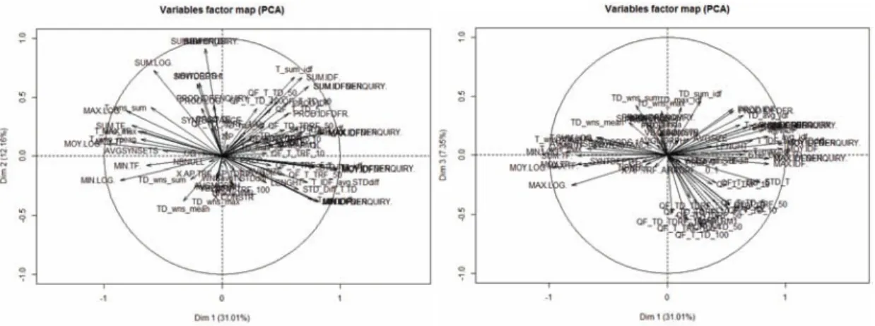
Clustering using PCA coordinates To solve feature scaling issues, or low feature variability from one query to another, we performed a principal component analysis (PCA) on the data.
Then we look at the variable coordinates in the first three dimensions, viewing the correla-tion circles (Figure 3). Even if the plots are not easily readable, we can extract some relevant information detailed below. If we look at the horizontal axis on the Figure 3, which corresponds to the first dimension of the PCA, we can see that there are, on the left side, variables related to the query features LOG and TF (term frequency in the collection). On the right side, we can find characteristics such as the inverse document frequency (IDF) and the normalised inverse document frequency (IDFN).
Fig. 3. Variables in the three dimensions of the PCA: dim1/dim2 on the left, dim1/dim3 on the right.
7
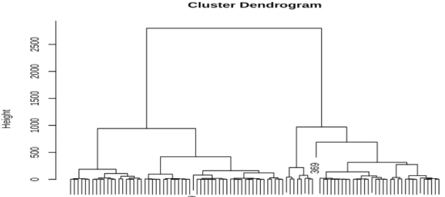
378 381 397 442 354 440 389 435 357 404 370 401 421 376 394 443 412 448 391 413 416 410 425 418 431 387 446 362 393 436 375 390 445 409 437 355 363 385 384 432 398 372 388 359 366 415 430 386 383 450 396 414 422 434 438 360 426 428 392 364 403 395 417 367 379 424 369 420 352 380 374 351 400 373 407 427 439 382 419 358 371 449 402 408 405 447 411 433 356 423 365 377 361 441 444 368 353 429 399 406 0 500 1000 1500 2000 2500 Cluster Dendrogram hclust (*, "ward") distE2^2 Height
Fig. 4. Dendrogram of the PCA coordinates (Ward’s method)
Considering the second dimension (left side graph), there are, on the upper side, character-istics SUM(TF_Q), SUM(LOG), SUM(IDFENQUIRY) and NBWords. On the lower side, charactercharacter-istics concern the terms ambiguity and minimum inverse frequencies.
Finally, the third dimension (right side graph) differentiates characteristics that measure the similarity between original and extended queries on the lower side, from characteristics that measure ambiguity of the extended query on the upper side.
From the new coordinates, we compute the Euclidean distance matrix and the hierarchical clustering. We opted for Ward’s for the agglomeration criterion: this method tends to give equal sized clusters (see Figure 4).
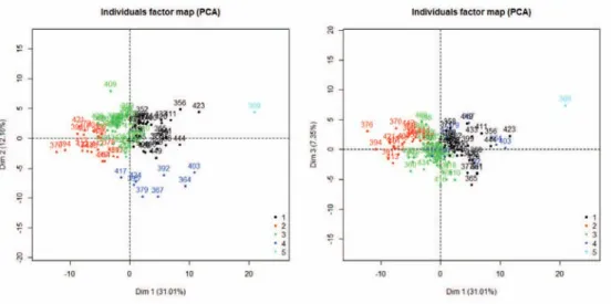
To choose how many clusters to keep, we plotted the height of the dendrogram branches against the number of clusters. Keeping 5 clusters seemed appropriate because it allowed us to have enough groups so that data sets would not be too large, but not too many so that there would be enough queries inside each group. It is possible to graphically represent the five clusters, using the axes defined by the PCA (see Figure 5). We can see that clusters 1 to 3 are not very different when we consider their coordinates on the vertical axes. Cluster 2 seems to be the one for which queries have the greatest LOG and TF whereas cluster 1 is the one where queries have a great inverse frequencies.
The majority of queries are assigned to three clusters (containing 33, 20, and 38 queries respectively). The fourth and the fifth clusters contain only 8 queries and 1 query, respectively. Therefore these queries are not included in the statistical analysis that follows.
Classification and regression trees As in Section 4.1, we study CART on queries from the first 3 clusters as defined by the query features. We also defined goodness of MAP values the same way as before, by using quartiles. We wanted to know what the best discriminating parameters were when considering query features rather than query difficulty; focusing on combinations of parameters that would give "good" results.
Cluster 1. Figure 6 shows that the parameters which best discriminate the goodness of MAP values are TrecQueryTags_process and retrieving_model. However, using a smaller complex-ity penalisation (a method parameter cp=0.0005) did not lead to "good" results with this tree.
Fig. 5. Five clusters in the PCA coordinates
Fig. 6. Classification tree for queries from Cluster 1
Cluster 2. The most important variables for the second cluster are retrieving_model and TrecQueryTags_process. CART for cluster 2 were not able to predict "good" results either, even when we changed the penalisation.
Cluster 3. For the last cluster, the most important parameters are the same as the ones of the two other clusters: TrecQueryTags_process and retrieving_model. There were no "good" predictions with this cluster either.
The most important variables that we have observed with these trees are the same as those obtained when we considered the level of difficulty of the queries (see Section 4.1). This means that parameters TrecQueryTags_process and retrieving_model are indeed very important in the prediction of the MAP values. However, with any of these trees, it was not possible to find the parameter combinations which yields "good" results. We changed the training set and the complexity penalisation ("cp") several times, but still without any "good" predictions. The cause might be the high number of "average" results in the data (twice as many as "good" or "bad" results)
Random Forests As previously, we use random forests and this method was applied on 10,000 random rows of each of the three query clusters and 500 trees were computed. By plotting graphs of accuracy, we saw that the accuracy was the greatest when there were four variables in the trees, no matter what the cluster was. We computed the parameter importance for MAP goodness prediction using the mean decrease in accuracy for each cluster.
First of all, for all three clusters, the most important parameters are the same; but in different order (retrieving_model, TrecQueryTags_process and trec_qe_model). Moreover, these pa-rameters are basically the same as the ones we obtained with difficulty clusters (see Section 4.1). Therefore, it seems like the kind of clustering we use does not have a significant influence on what the most important search parameters are. Alternatively, it could also mean that it is not necessary to divide queries into clusters, in order to know what parameters are the most important.
From the 10,000 observations used in the random forest we randomly choose 7,000 as a test set to check the prediction quality of our model. The error rates obtained from the confusion matrices are high, especially with "good" and "bad" predictions (0.74-0.76). On the other hand, for the "average" predictions the error rates are around 0.50. This difference between errors is due to the greater number of "average" MAP results in the training set. Therefore, it is easier for the model to predict "avg" results. However, even for average MAP results, the error rates are still very high. For this reason, it will not be possible to know for sure what parameter values should be used in order to get good MAP values.
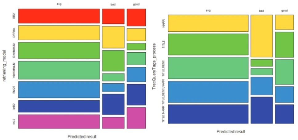
Fig. 7. Mosaic plots for Cluster 1 (retrieving_model and TrecQueryTags_process)
To get a graphical idea of what values to choose, we use mosaic plots on the training set pre-dictions. Therefore, for a given search parameter, we can compare the proportions of each value in every MAP goodness category. If the proportion of a specific algorithm in the "good" predictions is much greater than its proportion in the "average" and "bad" predictions, it could mean that this algorithm gives better MAP results, or at least it does so for the computed model. Mosaic plots are only reported with the two previous most important variables: retrieving_model and TrecQueryTags_processfor each of the three clusters (see Figure 7 for the first cluster).
From the presented graphs, one can notice that, in the "good" predictions of Cluster 1, there are moreInL2 algorithms than for the other levels of satisfaction. On the other hand, there are less DirichletLM algorithms than in "avg" and "bad" results (see left side graph). It could mean that InL2 is an algorithm that works better for queries that belong to the first cluster and that
it would be good to avoid the DirichletLM algorithm. Results are less obvious on the right side graph (TrecQueryTags_process). There might be a little bit more TITLE and TITLE,DESC in the "good" predictions than in the others, but we could say for sure that there are many more NARR fields used in the "bad" predictions. Therefore, it is probably a good idea to avoid using this field in order not to get too bad MAP values.
Using the same kind of arguments, it is possible to identify a few algorithms, for each cluster, that seem to be more present in the "good" predictions. Parameter values were very similar between the three clusters. Hence, it would seem like, to get good MAP results, one should choose the TITLE field (maybe also the DESC field) and avoid NARR. Moreover, retrieving algorithms InL2 and InB2 seem to give better results whereas it would be better to avoid DirichletLM algorithm.
Moreover, the results are to be considered in the light of error rates which were relatively high.
5
Conclusion
Search engines are tuned to perform well over queries. However, IR research has shown that there is not an optimal system that would answer the best on any query. Rather, system variability has been shown. The objective of this paper is to characterize query types and learn which system configuration is best for each query type. If we were able to do so, when an unseen query is submitted by the user, we would be able to decide which system configuration should process it. This implies first to define query types, then to learn the best system for each query type. In this paper, we defined two completely different types of queries. On each of these types, we analyzed which search parameters influence the most MAP and tried to find what values these parameters should be set to.
From a massive data set of more than 80000 system configurations, we found that two parame-ters (retrieving_model and TrecQueryTags_process) were quite influential. These parameparame-ters are the ones one should try to optimize first when optimizing a search engine. However, we show that it is very difficult to obtain conclusive results and that we were not able to learn the param-eter values that allow result optimization. This suggests that the query features used to assign query to systems might be not optimal. Yet, the parameters we used lean on various consideration from the literature of the domain, including many query difficulty predictors both linguistics and statistics that cover various difficulty aspects (term ambiguity, term discrimination, document list homogeneity and result lists divergence). The other reason for which the results were not enough could be that the learning functions we used do not fit the problem.
Regarding our future work we will try to adapt our findings to be used in the field of contextual IR, more specific in the selective IR. With improved models and better error rates, statistical tests would need to be performed to compare parameter values and to decide what values to keep to get good MAP values.
This study has used the MAP as the system performance measure. This measure is used when global evaluation is made. However, some other measures are more task oriented. For example, high precision measures the precision when considering the top retrieved documents, while some other measures are more recall oriented. It would be interesting to analyze if when considering different goals (recall/precision or other) results differ.
Acknowledgments. We would like to acknowledge the French ANR agency for their support through the CAAS-Contextual Analysis and Adaptive Search project (ANR- 10-CORD-001 01).
References
1. Banks, D., Over, P., Zhang, N.F.: Blind men and elephants: Six approaches to trec data. Information Retrieval, Springer 1(1-2) (May 1999) 7–34
2. Chrisment, C., Dkaki, T., Mothe, J., Poulain, S., Tanguy, L.: Recherche d’information. analyse des résultats de différents systèmes réalisant la même tâche. ISI 10(1) (2005) 33–57
3. Mizzaro, S.: Hits hits trec: exploring ir evaluation results with network analysis. In: Proc. 30th Int. ACM SIGIR Conf. on Research and Development in Information Retrieval. (2007) 479–486 4. Dinçer, B.T.: Statistical principal components analysis for retrieval experiments: Research articles.
Journal of the Association for Information Science and Technology 58(4) (February 2007) 560–574 5. Compaoré, J., Déjean, S., Gueye, A.M., Mothe, J., Randriamparany, J.: Mining Information Retrieval Results: Significant IR parameters. In: Advances in Information Mining and Management. (October 2011)
6. Harman, D., Buckley, C.: The NRRC Reliable Information Access (RIA) Workshop. In: Proc. 27th Int. ACM SIGIR Conf. on Research and Development in Information Retrieval. (2004) 528–529 7. Harman, D., Buckley, C.: Overview of the reliable information access workshop. Information
Re-trieval, Springer 12(6) (2009) 615–641
8. Mothe, J., Tanguy, L.: Linguistic features to predict query difficulty. In: ACM SIGIR 2005 Workshop on Predicting Query Difficulty - Methods and Applications. (2005)
9. Jones, K.S.: A statistical interpretation of term specificity and its application in retrieval. Journal of Documentation 28 (1972) 11–21
10. Shtok, A., Kurland, O., Carmel, D.: Predicting query performance by query-drift estimation. In: 2nd International Conference on the Theory of Information Retrieval. (2009) 305–312
11. Zhou, Y., Croft, W.B.: Query performance prediction in web search environments. In: Proc. 30th Int. ACM SIGIR Conf. on Research and Development in Information Retrieval. (2007) 543–550 12. He, B., Ounis, I.: University of glasgow at the robust track- A query-based model selection approach
for the poorly-performing queries. In: Proc. Text REtrieval Conference. (2003) 636–645
13. Kurland, O.: Re-ranking search results using language models of query-specific clusters. Information Retrieval, Springer 12(4) (August 2009) 437–460
14. Wen, R., J., Nie, Y., J., Zhang, J., H.: Query clustering using user logs. ACM Trans. Inf. Syst. 20(1) (January 2002) 59–81
15. Bigot, A., Chrisment, C., Dkaki, T., Hubert, G., Mothe, J.: Fusing different information retrieval systems according to query-topics: a study based on correlation in information retrieval systems and trec topics. Information Retrieval, Springer 14(6) (2011) 617–648
16. Mothe, J., Tanguy, L.: Linguistic analysis of users’ queries: Towards an adaptive information retrieval system. In: Signal-Image Technologies and Internet-Based System. (2007) 77–84
17. Kurland, O., Shtok, A., Hummel, S., Raiber, F., Carmel, D., Rom, O.: Back to the roots: A proba-bilistic framework for query-performance prediction. In: Proceedings of. CIKM ’12 (2012) 823–832 18. Chifu, A.: Prédire la difficulté des requêtes : la combinaison de mesures statistiques et sémantiques
(in French). In: Proceedings of CORIA, Neuchatel, Switzerland. (April 2013) 191–200
19. Voorhees, E.M., Harman, D.: Overview of the sixth text retrieval conference (TREC-6). In: Proc. Text REtrieval Conference. (1997) 1–24
20. Maxwell, S.E., Delaney, H.D.: Designing Experiments and Analyzing Data: A Model Comparison Perspective, Second Edition. 2 edn. Routledge Academic (2003)
21. Breiman, L., Friedman, J.H., Olshen, R.A., Stone, C.J.: Classification and Regression Trees. Wadsworth (1984)