Dynamic collision reduction protocol for ultra-wide bandwidth multiple access networks

-A

Dynamic Collision Reduction Protocol for Ultra-Wide

Bandwidth Multiple Access Networks

by

Gregory John Tomezak

Submitted to the Department of Electrical Engineering and Computer Science

in partial fulfillment of the requirements for the degree of

Master of Science in Electrical Engineering

at the

MASSACHUSETTS INSTITUTE OF TECHNOLOGY

May 2004

L

@

Massachusetts Institute of Technology 2004. All rights reserved.

A u th or ...

Department of Electrical Enginecring'and Komputer Science

May 21, 2004

C ertified by ...

VIoe Z. Win

Charles Stark Draper

sistant Professor

Thesis Supervisor

Accepted by...

Arthur

C. Smith

Chairman, Department Committee on Graduate Students

MASSACHUSETTS INST-ITUTE.

OF TECHNOLOGY

JUL

2

6

2004

Dynamic Collision Reduction Protocol for Ultra-Wide Bandwidth

Multiple Access Networks

by

Gregory John Tomezak

Submitted to the Department of Electrical Engineering and Computer Science on May 21, 2004, in partial fulfillment of the

requirements for the degree of Master of Science in Electrical Engineering

Abstract

In this thesis, we provide a cross-layer analysis of the throughput of the dynamic collision reduction (DCR) protocol, a multiple access protocol that requires frame synchronization. At the physical-layer, we develop the optimal neighbor detector for ultra-wide bandwidth (UWB) signaling in a dense multipath environment with delay uncertainty. The detec-tor takes advantage of the inherent multipath diversity associated with UWB signaling. We then develop an effective distributed control policy, derived from a dynamic program-ming formulation, to increase the throughput of UWB random-access networks in the DCR protocol. Finally, we construct a model for the distribution of nodes in the plane enabling closed-form analysis of two-hop signaling over wireless channels while capturing many of the transmission dependencies between randomly located relaying nodes. Our results demon-strate promising throughput.

Thesis Supervisor: Moe Z. Win

Acknowledgments

I would like to thank my advisor, Moe Win, for supervising this research and providing

di-rection. I would like to thank Andrew Brzezinski for many insightful conversations, reading drafts of this research, and providing valuable feedback. Additionally, I appreciate Marco Chiani for his time and valuable discussions.

My family has been amazing through my educational journey. My parents were

incred-ibly supportive and provided excellent direction. My wife was extremely understanding of the pressures and time commitments of a graduate student while I was at MIT. Finally, to my daughter, who was born towards the end of my studies, I appreciate her keeping me awake at night, encouraging research at all hours. I am thankful for their support.

Contents

1

Introduction 9

2 Overview of the DCR Protocol 13

3 Physical Layer Model and the Optimal Neighbor Detector 15

3.1 UW B Channel M odel ... 15

3.2 UWB Signaling ... ... 17

3.3 Optimal Neighbor Detector ... ... 19

4 Collision Reduction Control Policy 21 4.1 Formulation for Optimal Policy ... . 22

4.2 Formulation and Derivation of Sub-Optimal Policy ... 24

5 Two-Hop Signal Model and Analysis 27 5.1 Node Distribution and Two-Hop Signaling Model . . . . 27

5.2 The Probability that a Node Advances . . . . 29

6 Numerical Results and Discussion 33 6.1 Optimal Neighbor Detector ... ... 33

6.2 Collision Reduction Policies ... ... 35

6.3 Two-Hop Signaling Model . . . . 39

6.4 System Performance . . . . 42

7 Conclusions 45

List of Figures

2-1 The signaling slots of the DCR protocol. The nodes are pruned through N contention-echo slot (CES) pairings. . . . . 13

3-1 PAM-TH Ultra-Wide Bandwidth Signal. . . . . 18

5-1 Nodes x and y relay a signal from node z to node v. Relaying signals in a wireless setting may result in many intricate transmission dependencies between nodes. . . . . 28 5-2 In the model outlined above, each square contains one node. The location of

the node is uniformly distributed within the square, thus the node is equally likely to be anywhere within its square. The sixteen nodes in the shaded region are within two-hops of node z. Under this model, the locations of the nodes can be viewed as a quantization of the uniform distribution for the nodes in the plane. . . . . 29 5-3 Contending Node z will advance to the next CES pairing for the four events

above. Note that for the two branches that terminate with advances(F) erroneous communications results in node z advancing when this node should have been pruned in the kth contention slot. . . . . 32

6-1 The receiver operating characteristics at various SNRs and number of users. M= 90,Lp = 5,mk = l and Q2= 1 for k= 1, ... ,Lp and a uniform PDP

w as used. . . . . 34

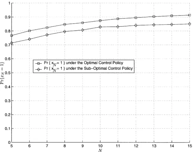
6-2 The probability that only one node remains after N CES pairings is plotted for both the optimal control policy produced by the dynamic programming recursion in (4.6) and the sub-optimal policy in (4.10), where xO = 100. . . 36

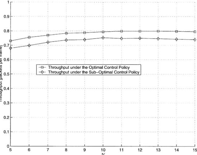
6-3 The signaling overhead due to the pruning process is N . The throughput is also included under both control policies for = 0.01, where the probability

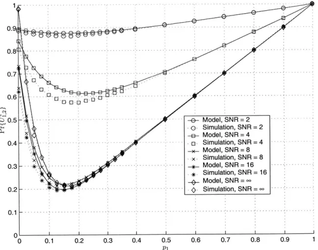
Pr{XN = 1} is shown in Fig. 6-2. . . . . 37 6-4 The probability that a contending node continues from the first to the

sec-ond CES pairing is plotted for various SNRs; it is observed that the model outlined in Chapter 5 is effective. . . . . 40

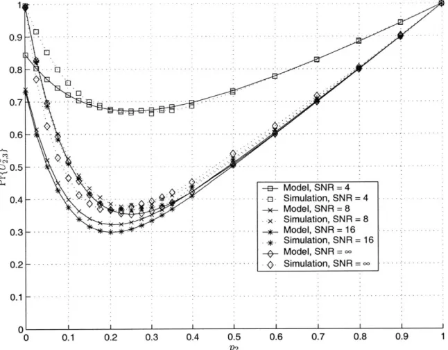
6-5 The probability that a contending node continues from the second to the

third CES pairing is plotted for various SNRs. It can be seen that the model remains effective with the independence approximation. . . . . 41

Chapter 1

Introduction

Coordinating nodal transmissions in mobile distributed wireless networks presents many challenging problems. Numerous channel access protocols have been proposed and devel-oped for use in mobile distributed wireless networks, and the topic remains an active area of research. Dynamic sharing of the channel, sometimes referred to as random-access, can be achieved through either asynchronous or synchronous means. Asynchronous schemes, like pure Aloha [1] or the carrier sense multiple access (CSMA) protocol [10], allow nodes to operate without any common timing reference. Synchronous schemes, on the other hand, require tightly synchronized clocks among the nodes and impose a timing structure so that transmissions may begin only at well known times, such as slotted Aloha [15] or CSMA slotted Aloha.

Slotted Aloha has been thoroughly investigated in the literature. The throughput for sta-bilized slotted Aloha with Poisson arrivals has been shown to be approximately 1/e ~ 0.368 packets per slot [2,5]. To improve the throughput of slotted Aloha, many sophisticated col-lision resolution techniques have been developed, including a variety of splitting algorithms (see for example [14]). With these advances in slotted Aloha, throughput is still upper-bounded by 0.587 packets per slot [13], where splitting algorithms have obtained through-puts of approximately 0.5 packets per slot [19]. In the effort to increase throughput, other contention protocols have been proposed. The synchronous unscheduled multiple access protocol shows promise in attaining higher network throughput, in addition to providing fairness properties and overcoming the hidden terminal problem [8].

multi-hop wireless environment, including the classic works [10, 17,18]; many interesting models and topologies have been presented. When nodes are randomly distributed in a plane according to some probability distribution, intricate transmission dependencies exist be-tween the nodes relaying a signal in a wireless environment. However, accurately capturing these dependencies in a model presents a significant challenge. Additionally, the research within network-layer communities and physical-layer communities has only recently moved towards cross-layer system analysis. That is, in typical network-layer research, focusing on network-layer issues such as throughput or delay, works are only now beginning to incorpo-rate realistic physical-layer constraints. In understanding the performance of network-layer metrics, consideration of physical-layer limitations needs to be addressed, so that these limitations are accounted for in overall system performance.

Throughput in a contention based protocol can be improved using a stochastic decision making policy to dynamically adjust the process at which nodes compete for uncontested channel access. This adaptive control policy maximizes the probability that only one user transmits in the data frame thus avoiding collisions. Dynamic programming techniques, (see for example [4]), may be applied to such a problem. Often, dynamic programming techniques do not lend to analytically tractable solution of the control policies, so sub-optimal approaches are considered for real-time distributed applications.

In this thesis, we propose a protocol, named the dynamic collision reduction (DCR) protocol. The DCR protocol reduces channel access collisions among nodes within two-hops of each other by taking advantage of distributed stochastic decision making policies, which incorporates physical-layer and network-layer considerations. The neighbor detector was designed for ultra-wide bandwidth (UWB) signals in a multipath fading environment. The inherent multipath diversity and the low probability of detection and interception [21-25] make UWB signaling attractive for reliable and covert communications.

We then develop a distributed dynamic decision making policy to increase throughput of UWB random-access networks. First, we formulate the dynamic programming recursion that provides the optimal policy to maximize the throughput. Since closed-form expressions for the optimal control policy are difficult to find, sub-optimal approaches are developed for distributed real-time application in DCR to increase throughput. The DCR protocol enables nodes that are separated by two-hops to effectively compete against each other for transmission rights. Thus, a possible collision at a node, which is common to both

competing nodes, is avoided. To capture realistic wireless scenarios pivotol in the design of the control used in DCR, we formulate a model that captures the transmission dependencies between the randomly distributed relaying nodes in a two-hop wireless setting. The analysis is truly cross-layer in the sense that it encompasses the fields of detection theory, network probabilistic models, and sequential decision making in the presence of uncertainty.

This thesis is organized as follows. In the next chapter, we provide an overview of the operation of the DCR protocol. In Chapter 3, we present the channel model and derive the optimal neighbor detector. In Chapter 4, we analyze the appropriate distributed control policy undertaken by each node. We formulate and examine the model used to characterize two-hop signaling in a wireless network with randomly distributed nodes, in Chapter 5, which is imperative in obtaining the throughput. In Chapter 6, we provide numerical results and discuss the relationships between the proceeding chapters. Finally, Chapter 7 consists of concluding remarks.

Chapter 2

Overview of the DCR Protocol

In the DCR protocol, each data frame consists of a series of signaling slots followed by the data slot, as shown in Fig. 2-1. The active nodes compete for the right to transmit through the use of the signaling slots, motivated by the synchronous unscheduled multiple access protocol [8]. Unlike traditional access schemes that use control frames to indicate available data to transmit, the DCR protocol requires that a contending node transmit only a single bit to indicate the node's intent to transmit data. This type of contention requires clock synchronization between the nodes; the limitations of this synchronization will be accounted for in the design of the neighbor detector.

The signaling slots are comprised of N contention-echo slot (CES) pairings, where the number of contending nodes will be pruned down such that only a single node has uncon-tended access to the channel. A contention slot is always immediately followed by an echo slot. Each node vying for access to the channel will transmit a signal in the kth contention slot, Ck, with probability Pk. Each node in the network will listen for a transmitted sig-nal(s) from the neighboring node(s). Any node that detects the presence of a signal from a neighboring node, in addition to all contending nodes that transmitted in the contention slot, will transmit a signal in the corresponding echo slot, Ek.

Only a contending node in the kth CES pairing can advance to the (k + 1)th CES pairing

C1 El C2 E2 CN EN Data Packet ACK

Figure 2-1: The signaling slots of the DCR protocol. The nodes are pruned through N contention-echo slot (CES) pairings.

as a contender. The contending node will continue if either of the following two events occur:

* The contending node transmits in the kth contention slot.

* The contending node does not transmit in the kth contention slot and does not detect

a signal in either the kth contention or echo slots.

The former occurs with probability Pk while the probability of the latter is examined more closely in Chapter 5. It is important to note that Pk is not necessarily the same for all contention slots and is a parameter that can be altered at each CES pairing.

If, for example, contending node z does not transmit in the kth contention slot, does not detect a signal in the kth contention slot, and then detects a signal from a neighboring node in the corresponding echo slot, this node will not advance to the (k + 1)th CES pairing. In

this example, one or more nodes that are two-hops from node z were responsible for node z being pruned at the kth pairing. Thus, a node that is possibly "hidden" can effectively compete for the opportunity to transmit data because of the signals being relayed in the echo slot. In this fashion, the DCR protocol prunes down the number of nodes which can transmit so that communications occur in a relatively collision free environment.

Chapter 3

Physical Layer Model and the

Optimal Neighbor Detector

The transmission of extremely short duration pulses occupying immense bandwidths has been known since the 1960s in the RADAR community [16]. Over the past few years, a great deal of interest has been given to adopting these signals for various wireless communica-tions applicacommunica-tions, refered to as UWB signaling [21-25]. Recently, the United States Federal Communications Commission (FCC) has approved transmission of UWB signals while con-trolling interference in licensed spectrum [7]. Because of the fine time resolution provided by UWB signals, one is able to exploit the inherent diversity associated with multiple distinct paths reaching the receiver. Additionally, the low probability of interception and detection, which is fundamental to UWB, makes this form of signaling even more attractive. Because of these properties, UWB is adopted for reliable and covert communications. It is natural, therefore, to also consider UWB for the signaling slots of the DCR protocol to exploit these properties. In this section, we present the channel model followed by the optimal neighbor detector.

3.1

UWB Channel Model

UWB signals occupy immense bandwidths, inversly proportional to the duration of a single pulse, which results in excellent inultipath resolution [22,23,25]. The number of multipaths, LP, for each user depends on the operating environment. For example, in an indoor envi-ronment LP would be large, while an outdoor envienvi-ronment with a small number of scatters

would have a relatively small LP. Therefore, the received signal consists of the superposition of Lp resolvable components, where each component is weighted by the fading amplitude and phase associated with the wireless environment.

In order to construct a detector that will utilize the resolvable components of the received signal, we begin by discretizing the time axis. We consider each bin to have duration

A seconds, where A is inversely proportional to the transmission bandwidth. Therefore,

two multipath components within different delay bins are distinguishable. However, two multipaths within the same bin are unresolvable. A multipath with delay -T is contained within the

j

th bin, which is

jA

seconds after the nominal delay for that signal.

After a communication link at the network-layer has been established, synchronization at the physical-layer can be maintained between the two nodes. During each of the signaling slots in DCR, however, a contending node transmits only one symbol to contend for the channel. Thus, due to the random location of the nodes in addition to time offsets from

GPS shortcomings, the delay of the first arriving multipath is unknown at the receiver. We

consider M + LP - 1 different time bins, where the delay of the first arriving path of the signal is equally likely to be in any of the first M bins. Furthermore, we consider a dense multipath channel in which the next LP - 1 distinct paths of the signal at the receiver will

occupy the Lp - 1 time bins immediately following the first path. Thus, if the first path is

in the Jth bin, then each successive time bin will contain a received path with bin j + LP - 1 containing the last resolvable path.

In detecting the superposition of LP distinguishable multipath components, the perfor-mance of the receivers exploiting multipath diversity depend on the signal-to-noise ratio (SNR) at each branch in the receiver. This relates to the normalized power at the branches, commonly referred to as power dispersion profiles (PDP) [6]. The PDPs have been devel-oped based on channel measurements in various environments. The amount of energy in the bins of each multipath is determined by the PDP for the given environment; thus, the kth multipath of the received signal, where the first path is contained within the jth bin,

has energy Ej,k. For example, all Lp paths would have the same energy for a uniform PDP. The fading amplitude of the kth path is denoted with 0

ak. We consider independent non-identically distributed (i.n.i.d.) Nagakami-m fading for each path having second moment

Q' and parameter Mk. In the case of UWB transmissions, with no sinusoidal carrier, the baseband signal is entirely real and the random phase simplifies to either wholly unaffecting

the received signal or inverting the received signal. Thus, the random phase of the kth multipath, 0

k, assumed to be independent and identically distributed (i.i.d.) along each path, will take values of either 0 or 7r radians with equal probability. Furthermore, the fading amplitude and phase are taken to be mutually independent. Finally, we consider additive noise. The noise, n(t), is assumed to be zero-mean, white Gaussian noise with two-sided power spectral density (PSD) No/2.

3.2

UWB Signaling

In UWB communications, one symbol is comprised of several short duration pulses. The data symbol can be modulated using either pulse position modulation (PPM) or pulse amplitude modulation (PAM). In this thesis, we consider time-hopping (TH) PAM signaling, where TH provides security measures intrinsic to the randomness of the TH sequences [21,241. The transmitted TH-PAM signal for a given symbol of the eth user can be written as

Ns-1

s() d()p(t - jT - cgeTc), (3.1)

j=O

where p(t) is the basic signal, referred to as a monocycle which has duration Tp. For PAM,

{

d() is chosen from M amplitudes remaining the same for all N, pulses, where log2 M

bits per symbol are transmitted. The frame size for each monocycle is denoted by Tf; thus, the transmission of the symbol is of duration NsT. To provide multiple access and security measures, each monocycle is then offset an additional amount c TC. Each user is assigned a

psuedo-random sequence, {ce}, known only to the transmitter and receiver. Furthermore, to avoid interpulse interference, 0 < V Te < T.

In the DCR protocol, each node receives the signal(s) from the neighboring contending node(s). However, each receiving node only needs to detect the presence of at least one con-tending node vying for the channel; a receiving node does not need to make any distinction between different contending nodes. Thus, since no differentiation between users is needed in the signaling phase, all nodes will use the same psuedo-random TH code,

{cj

}.

Since the nodes are randomly distributed in the plane with internal clocks that are not perfectly synchronized, in addition to being mobile, the exact delay of the signal is unknown

S(t)

A

000

AA

Tf 2_Tf

3Tf (NS-1)T . NsTf

cITe _c2Tc

Figure 3-1: PAM-TH Ultra-Wide Bandwidth Signal.

at the receiver. This motivates the adoption of On Off Keying (OOK), i.e., d(') = 0 or 1,

instead of PPM for application in DCR. OOK was implicit in the discussions of the DCR protocol when there was mention of a node just detecting a signal from a neighboring node.

The received signal for Lu users and Lp multipaths for each user is given by'

L, LP

r(t) = afX e-ike ,ks((t - Te,k) + n(t) f=1 k=1

N, -1

where s(e)(t) = d(tp(I - jT - cjTc). (3.2) j=0

An example of s(t) representing a UWB symbol is shown in Fig. 3-1.

We derive the receiver below for the case where there is only one user. We address the issue of several nodes transmitting in Chapter 6. For one user transmitting, consider the following two hypotheses: under 70, the received signal is noise, while under H1, the

received signal is the superposition of the LP multipaths of the transmitted signal with additive noise. Therefore,

rn(t) udrN

r(t) = _{under Ho (3.3)}

E l

Z

cke-fk Z' sjk (t - Tj+k-1)

+ n(t)

under

H

1,

where we have normalized the energy of the transmitted signal, so that 9(t) = s(t) Mt-The Neyman-Pearson criterion is employed to derive the optimal detector for the re-ceived signal in (3.3). We will show in Chapter 5 that the choice of the maximum tolerable probability of false alarm is highly valuable in obtaining the throughput of DCR. The

portance in the choice of the false alarm probability is the motivation for the usage of the Neyman-Person criterion as opposed to the Bayes criterion.

3.3

Optimal Neighbor Detector

For the Neyman-Pearson criterion, the optimal test compares the average likelihood ratio, E{A[r(t)]}, to a threshold. The averaging is performed over the random phase and fading amplitude of each path and the delay of the first multipath. As shown in the Appendix A,

IM LP E{A[r(t)]} = M Lf Yj,k (3.4) j=1 k=Sl where S

)M

exp V

jk

IF(mnk) (Mk + E,kQk Ck X D-2Mk Vk

+

D--2rk ' ,k

(

vCj,k (-j,k

1

Mk~ +~Jk

2~m

+~j VNCjk

/

Cj,k = k+ Eo _, and Vj,k = 2 k r(t)s(t-Tj+k-I)dt. For the Neyman-Pearson criterion, there is a predetermined maximum allowable probability of false alarm, PFA, denoted by /, which allows for the evaluation of the threshold, A, to which the likelihood ratio is compared. This threshold is then used in the determination of the probability of detection, PD. Thus,

PFA = PrIE{A[r(t)]} > A I Ro} < 3. (3.5)

Using the threshold, A, generated in (3.5),

PD = Pr{E{A[r(t)} > A I H1 . (3.6)

Closed form expressions for the cumulative distribution function (CDF) of E{A[r(t)]} under either hypothesis are not known. We simulate the receiver operating characteristics and discuss other aspects of the neighbor detector in Chapter 6.

The limitations of the physical-layer signaling over a harsh wireless environment can now be considered in conjuction with the development of the network-layer analyses. We

next develop the stochastic decision making policy that ensures high throughput before developing a model to understand the transmission dependencies of relaying nodes when the nodes are randomly distributed in the plane.

Chapter 4

Collision Reduction Control Policy

In any contention based protocol, the ultimate objective is to guarantee only a single user permission to transmit and thus provide uncontended access to the channel for that user. In this chapter, we propose a stochastic decision making policy that ensures high throughput in DCR. The purpose of the policy is to ensure that only a single user remains at the end of the N stage pruning process. The policy controls the system through the selection of the probability that an arbitrarily chosen node continues to the next CES pairing.

In Chapter 5, we will show that the probability that an arbitrarily selected node advances to the next CES pairing is a function of the probability that a node transmits in the contention slot, the probability of false alarm, and the probability of detection, which itself is a function of the maximum tolerable probability of false alarm through the Neyman-Pearson criterion. Thus, through Pk and PFA,k, the probability of false alarm at the kth

CES pairing, the probability that a node will advance to the (k + 1)th stage can be specified.

Throughput is maximized when the probability that only a single user remains after the N stage pruning process is maximized, which can be accomplished by appropriately choosing the probability that a contending node advances at each stage.

A random number of nodes are pruned at each stage according to some distribution;

therefore, any a-priori selection of the probabilities that a node will continue at each stage does not take advantage of the information about the number of nodes pruned in the pre-vious stage. We assume that each node has perfect knowledge of the number of contending nodes in the network. While this assumption is difficult to implement, one could ascertain an estimate of the number of contending nodes in the network and employ this value as if

it were the actual number of contending nodes. This assumption is similar to that taken by the original researchers of Aloha; it was not until [12] that an adequate method of estimating the state of the backlog was known.

4.1

Formulation for Optimal Policy

Dynamic programming is an optimization technique to solve sequential decision making problems, whereby the optimization results in the minimization or maximization of the expected summation of the cost at each stage,

E {N(XN)+ N9k(i Uk,Wk) , (4.1)

k=O

where N is the horizon, Xk is the state of the system, Uk is the control, Wk is the random disturbance, gN(XN) is the terminal profit or cost, and gk(xk, Uk, wk) is the profit gained or the cost incurred at the kth stage [4]. More specifically, in our system, Xk is the number of contending nodes at the beginning of the kth contention slot. The state of the system is controlled by Uk, the probability that a contending node continues from the kth to the (k + 1)th CES pairing. The random disturbace, Wk, is the number of nodes pruned at the kth CES pairing and N is the number of CES pairings.

We relate dynamic programming to the maximization of the probability that only one user transmits with the following indicator random variable,

IXN N (4.2)

0 if xN I

Thus, with probability Pr{XN =1, XN takes on value 1. To maximize Pr{XN = 1}, we

could equivalently maximize E{IXN}. Let gk(xk, Uk, wk) = 0 for all Xk, Uk, Wk and k =

0,1,...,N- 1, and

9N(XN) = 1 if XN 1 (43)

-Therefore, dynamic programming will produce the optimal control policy,

7r= [o(xo),..., PN-1(XN-1),

that maximizes the expectation of the summation of the profit at each stage, namely E{IXN}, and thus maximize Pr{XN = 1}. The control at stage k is then given by Pk(Xk) A uk. To obtain this control policy, we must first develop the evolution of the state of the system and express the distribution of the random disturbance.

The number of nodes in the next stage is simply the number of nodes at the prior stage less the number of nodes pruned. Thus,

k+1 = Xk -Wk, k = 0, 1,.. ., N - 1. (4.4)

Note that the number of nodes pruned at the kth stage must be an integer within [0, Xk]. Thus, Xk+1 < Xk for all k = 1,... N - 1. Finally, to complete the dynamic programming

formulation, we express the distribution for the number of nodes prunded at the kth stage as,

Pr{wk = fx, Uk} = () (1 -U) Uk

for f = 0, 1,- .. , k and Xk _= 0, 1,.. ., o, (4.5)

where x0 is the number of nodes initially contending. In Chapter 5, we will explicilty express

the control, Uk, as a function of Pk, PFA,k, and PD,k, the probability of detection at the kth

CES pairing. The two-hop signaling model developed in the following chapter enables the

evaluation of this function. With this function and the determination of the control given by the dynamic programming formulation, each node is able to select the protocol controlled and physical-layer parameters, namely Pk, PFA,k, and PD,k to achieve the desired control.

The dynamic programming recursion now follows,

JN(XN) = 9N(XN)

Jk (Xk)= max Ek{Jk+1(Xk-wk)} k=0,1,...,N-1, (4.6)

UkE [, 11

Unfortunately, closed-form solutions for the control policy are difficult to derive, if pos-sible at all. Thus, in general, a function for pk cannot be obtained and the optimal control policy is usually found using simulation. This approach, while optimal, presents signifi-cant implementation challenges. Since a closed-form solution was not found for the optimal control policy, the dynamic programming algorithm must be computed "on-line" or in real-time. Numerical realization of dynamic programming cannot be accomplished "on-line" due to the large state, control, and disturbance spaces, often referred to the "curse of dimension-ality" [3]. Because of these limitations of dynamic programming, we consider alternative approaches to obtain closed-form solutions for the control policy.

4.2

Formulation and Derivation of Sub-Optimal Policy

Due to the practical limitations of implementing the control policy obtained in the previous section, we consider another formulation. We employ the same notation and variables as before, with the exception that in this section, we wish to minimize a cost as opposed to maximizing a profit. The evolution of the state and the distribution for the random disturbance remains the same. However, we choose a cost function that when minimized will increase the likelihood that XN = 1. We will consider a trajectory, (zi, .... ,

z),

where

XN =

L-The cost function is chosen that when minimized will force the state of the system to remain close to the ideal trajectory. It is important to note that the control policy that minimizes the cost function does not necessarily maximize the probability Pr{XN = zN} and thus throughput. Nevertheless, it seems intuitively clear that forcing the state of the system to remain close to the desired trajectory increases the likelihood that at the Nth stage the state of the system is

zN.

To force the state of the system to remain close to the ideal trajectory, we wish to heavily penalize the system for large deviations from the ideal trajectory and impose a small penality for small deviations from the ideal trajectory. Thus, a quadratic cost function is appropriate; the cost incurred at the kth stage is then,

We thus have the following dynamic programming recursion:

JN(XN) = (XN - XN)2

Jk(Xk) = min E,{(Xk - ) +Jk+1(Xk - wk)} k= 1,2,... ,N - 1. (4.8)

Uk [0,1]

A well known result in dynamic programming is the ability to obtain closed-form solutions

using the discrete-time Riccati equation when the system evolves linearly with a quadratic cost with unconstrained control

(4].

Since the control is constrained to be a probability, closed-form solutions do not exist. Therefore, to obtain a control policy, we examine some heuristic cost-to-go approximation. Consider a "near sided" heuristic whereby the future cost of the system is approximated by the cost in the following stage only. The future costs are minimal if the next state is close to the ideal trajectory and hence the approximation will perform well. Therefore,

JN(XN) = (XN - XN)2

Jk (Xk) =min E,,{(k - )2 +Hk+1(Xk - wk)} k= 1,2 ... ,N-1, (4.9)

UkG[0,1]

where Hj (x) = (x -

z

)2 for all

j

= 1, .. , N - 1 and HN(x) = JN(x) for all x. Therefore,

Jk(Xk) =min Ewk{(Xk k) + Hk±1(Xk - Wk)} Uk E [0,11

= (Xk - k )2 + min Ewk{xXk - Wk - Xk+1)2 Uk C[0,11

= (Xk - -k )2 + (Xk - k+1)2 + min 2E{w} - 2(Xk - -k+1)E{Wk}],

where E{wk} and E{wk} are the first and second moments of a binomial random variable with paramters, Xk and 1 - Uk. Therefore, minimizing XkUk(1 - Uk) + X 2(1 - uk)2 - 2(Xk

-'k+1)Xk(1 - Uk) with respect to Uk, we find its optimum value to be

24k+1 - 1

2(Xk - 1)

IfxkO ,x =1,or Xk < zk+1+1, then the corresponding control is not feasible. In these

cases, except Xk = 0, the optimal control will force the state of the system to remain the

protocol is

min[1, 1 ] if Xk > 1

Uk 1 if Xk =1

(4.10)

DNM if Xk = 0.

The control simply does not matter (DNM) if Xk = 0, as Xk+1 < Xk and thus it is now impossible for one node to remain by the kth stage. Discussion concerning the choice of the state trajectory and the performance of the sub-optimal approach is developed in Chapter 6. This chapter determined the selection of Uk to increase throughput; we must now determine how Pk, PFA,k, and PD,k are chosen to achieve the specified Uk.

Chapter 5

Two-Hop Signal Model and

Analysis

As seen from the previous chapter, the performance of the DCR protocol is highly depen-dent upon the probability that an arbitrarily chosen contending node continues from the kth to the (k + 1)th CES pairing. In this chapter, we provide a model that enables the

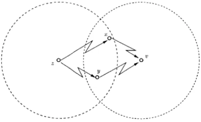
derivation of closed-form expressions for this probability. Nodes that are two-hops apart can compete against each other for transmission rights, through the echo slots. Thus, we must understand the manner with which randomly distributed nodes relay signals in a wire-less setting. Consider the following scenario: node z is two hops away from node v, where nodes x and y can provide the link between z and v. If node z contends for the right to transmit, both x and y can relay that signal to v in the echo slot, see Fig. 5-1. Particularly, when nodes are randomly distributed, there exist intricate dependencies between the nodes relaying signals in the echo slot. In this chapter, we present the two-hop wireless signaling model followed by the derivation of the probability that a contending node continues to the next contention-echo slot pairing.

5.1

Node Distribution and Two-Hop Signaling Model

We consider the following model for the means by which the nodes transmit and are dis-tributed in the plane:

I Ve

Figure 5-1: Nodes x and y relay a signal from node z to node v. Relaying signals in a wireless setting may result in many intricate transmission dependencies between nodes.

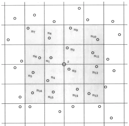
exactly f nodes, where the location of each node is positioned according to a uniform distribution in the square. Thus, while guaranteeing f nodes in each square, the location of the nodes within each square is random. In this chapter, we consider t = 1 node in each square. The analysis generalizes to f nodes in each square, although becoming cumbersome. Henceforth, we will refer to the node in square j as nj, as depicted in Fig. 5-2.

2. Each node can detect the presence of a signal transmitted by a node in any adjacent square. The node will detect a signal when it is present with probability PD,k and incorrectly detect a signal when it is not present with probability PFA,k in the kth contention and echo slots. The aim of this assumption is to provide a rough radius whereby any signal transmitted by a node outside of that radius cannot be detected. The size of the squares is ultimately dictated by the power at which the nodes transmit.

3. To avoid strange edge effects, we consider the nodal plane to be extremely large

relative to the size of a square. Furthermore, we assume that the node of interest is located at the intersection of the four squares in the middle of the plane, whereby it can only detect the nodes in those four squares. Thus, it is reachable in two hops from any node in the surronding sixteen squares, as shown in Fig. 5-2.

4. For the entire N stage pruning process, in addition to the actual data packet transfer, we assume that the locations of the nodes are static. In this paper, our goal is to increase the throughput limits in contention based protocols. Therefore, we make no further assumption on the movements of the nodes between frames since we are not

Figure 5-2: In the model outlined above, each square contains one node. The location of the node is uniformly distributed within the square, thus the node is equally likely to be anywhere within its square. The sixteen nodes in the shaded region are within two-hops of node z. Under this model, the locations of the nodes can be viewed as a quantization of the uniform distribution for the nodes in the plane.

5. In an implementable network using the DRC protocol, all nodes within two-hops of

a randomly chosen node influence the event that node z is still contending. However, the event that node z is contending at the kth pairing is approximately independent of the event that node y is also contending at the kth pairing. With this approximation, the probability that a contending node transmits in the kth pairing does not need to be conditioned on the past history of all nodes within the network for that given data frame.

5.2

The Probability that a Node Advances

As detailed in Chapter 2, a contending node will continue from the kth to the (k +

1)th

CES

pairing if either of the two events occur. The contending node transmitted in the contention slot, which occurs with probability Pk. Or, the contending node does not transmit and does

0 0 00 0 0 nn80 n _j 0 0 0 0n2 0 n6 0 _{n11 0} 0 n12 'n5 _n4 0 0 nlo 0 0 0 n15n1 n3

o

0 0 0 0 0

not detect the presence of another signal in either the kth contention or echo slots. Before expressing this probability, we adopt the following notation:

Uk',k+l athe event that contending node z continues from the kth to the (k

+

1)th pairing.

Wk a the event that node z is contending at the beginning of the kth contention slot.

T k the event that node z transmits in the kth contention slot. Dz EE the event that node z detects a signal in the kth contention slot.

ViA athe event that at least one of the nodes in A transmited in the kth

contention slot, where A is the set of all nodes within 1-hop of node z.

Thus, {V5 } ={T U... U Tj3 }. Note, that a node could also transmit or detect a signal in the kth echo slot, where similar notation would apply. In addition, throughout the analysis, an overbar will indicate the complement of the associated event; for example, Tgk is the event that node z does not transmit in the kth contention slot. Since each contending node that transmits in the kth contention slot also transmits in the corresponding echo slot, in addition to any node detecting a signal in the contention slot, the number of nodes transmitting in the echo slot is always greater than or equal to the number of nodes transmitting in the contention slot. However, the receiver design does not account for a different number of nodes transmitting. Thus, it is not necessary to distinguish between PD,k in the contention slot and echo slots.

Since detection errors are made at the physical-layer, the selected contending node will continue to the next pairing if any of the events are satisfied. Within the chosen model, all nodes will transmit independently in a contention slot. Furthermore, node z will correctly or incorrectly detect the presence or absence of a signal independently of the other slot,

when conditioned on the hypothesis. Using these relationships and Fig. 5-3, Pr{Ukz,k+I} = Pr{T } + Pr{k} Pr{Vc

}

Pr{Dk VC Pr{V T7, Vk Pr{DkVg

}

I ZkEk (5.1) +Pr Vkj Pr VC Pr- ( r{ | , P{ IV + Pr( Pr kj Pr

DF|(

Pr VE~ I T Pr{DkV (.

Simplifying the above expression,

Pr{Uk,k+l = Pk + (1 - pk)Pr{Vck

}

(1 - PDk)2

+ (1 -Pk)Pr{Vf} (1 -PFA,k)Pr{VLk T~kTk

+ (1 - Pk)Pr{

}

(1 - FFA,k)Pr 1 - PD,k). (5.2)

The probability that a node continues to the next CES pairing is computable if we can express Pr{Vg

}

and Pr{VgkIT6C C

},

regardless of the underlying model. We obtain these expressions in Appendix B.

Substituting (B.2) and (B.10) from Appendix B into (5.2), we have obtained a closed-form expression for the probability that a contending node continues to the next CES pairing. In Chapter 4, we ascertained a control policy that determines this probability if there exist Xk contending nodes in the system. Therefore, by determining PFA,k, which in turn fixes PD,k for a given SNR, Pk can be selected using (5.2) to achieve the control given

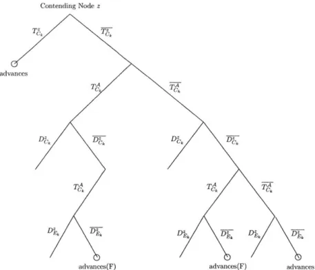
Contending Node z

TC4, _TKI

advances

TAC TA

advances(F) advances(F) advances

Figure 5-3: Contending Node z will advance to the next CBS pairing for the four events above. Note that for the two branches that terminate with advances(F) erroneous commu-nications results in node z advancing when this node should have been pruned in the kth contention slot.

Chapter 6

Numerical Results and Discussion

In this chapter, we present and discuss numerical results of the optimal neighbor detector, the collision reduction policies, the two-hop signaling model, and overall system perfor-mance.

6.1

Optimal Neighbor Detector

The expresions for the CDFs of E{A[r(t)} given Ho and H1 are not known. Therefore, we

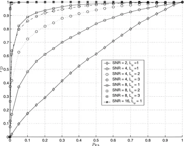
simulate the CDFs of E{A[r(t)} for each hypothesis. Simulation results for the performance of the neighbor detector at various signal-to-noise ratios (SNRs) are provided in Fig. 6-1 for M =90, LP = 5, mk =1 and Q2 = 1 for k = 1,..., Lp. In addition to these parameters, a uniform PDP was considered in this simulation. Recall that the neighbor detector is optimal for one node transmitting over a multipath fading channel, where the delay of the signal is unknown.

Although the optimal detector was derived for one node transmitting, several nodes could possibly transmit in a given contention or echo slot. It is worthwhile to note that the amount of signal energy detected in the case of multiple nodes transmitting is not always greater than the amount of signal energy detected in the case of only one node transmitting. It is probable, although unlikely, for the received signal energy of several nodes to add destructively at the receiver and therefore degrade receiver performance. Consider

00

o-SR=4L

= ... .. ... . .. .. .. ...,L = 0.1 -0.6 -1-a-.- .- . -.-SNR _{2, Lu o} ... -.. . . .. -... .. . S N R = 4 , Lu =1 . .. .. .. . . . . . SSNR = 4, L = 2 SSNR = 4, L = 3 0 .4 -. . . . . . .... . . .. . . ... . .. .. .E S N R = 8,L = 1 ... . .. ... .. . . u.SNR = 8, LU = 2 . .3 . . .. . . .-.-...-.- ...-... .. -.. . .. .- . . S N R = 8 , Lu = 3. . . . .. . . . . SNR = 16, Lu= 0 0.1 0.2 0.3 0.4 0.5 0.6 0.7 0.8 0.9 1 PFA

Figure 6-1: The receiver operating characteristics at various SNRs and number of users.

M = 90, LP = 5, mk = 1 and Q2 = 1 for k = 1, . .,Lp and a uniform PDP was used.

Lu nodes transmitting:

Pr{No collisions of the multipaths from the Lu contenders} M-(Lu -1)L p

{

if Lu Lp < M

0

otherwise.

With this probability, the energy received is the sum of the energies of all Lu nodes trans-mitting. As Lu increases, it becomes more likely that some paths will arrive in the same bin as other paths. This, however, does not imply that the signal energy will necessarily add destructively. Furthermore, if Lu is large, it is highly probable that the total received energy is greater than the energy received from just a single user. It was verified in simulation, where M, Lp, Mk, and Q2 were as above, in addition to the same PDP, that PD improves as the number of users transmitting increases, also seen in Fig. 6-1.

6.2

Collision Reduction Policies

In Section 4.1, the dynamic programming recursion obtained in (4.6) yields the optimal control policy. To obtain the optimal control policy through simulation, we begin by finely discretizing the control space. Then, at each stage for every possible state, the expected future profit is computed for each control. The control to maximize the expected future profit is the optimal control for that stage and state. We let the system evolve where the number of nodes pruned at the kth stage was chosen from the distribution provided in (4.5). Using the optimal control policy, we obtain the probability Pr{XN = 1}, as a function of N

for xO = 100, as seen in Fig. 6-2. Clearly, Pr{XN = 1} increases as N increases. It was also

seen in simulation that for a given N, Pr{XN = 1} remains the same for different values of

XO.

We consider an alternative dynamic programming formulation in Section 4.2 due to the implementation difficulties of solving the dynamic programming recursion "on-line." A difficulty with the sub-optimal approach lies within the choice of the state trajectory. The trajectory was chosen such that most of the initial contending nodes are pruned within the first two CES pairings. In the remaining pairings, the trajectory slowly approaches

zN

= 1, to lessen the risk of pruning all of the nodes and thus allowing the channel to remain idle.

0.9

0.8 0.7' 0.6

0.5

-a- Pr { xN= 1 } under the Optimal Control Policy Pr { xN= 1 } under the Sub-Optimal Control Policy

0.4-0

.3 --- - - -

----o.1

5 6 7 8 9 10 11 12 13 14 15

N

Figure 6-2: The probability that only one node remains after N CES pairings is plotted for both the optimal control policy produced by the dynamic programming recursion in (4.6)

and the sub-optimal policy in (4.10), where xo = 100.

0.9 [ - - .-.-V.2 0.1 0 E3E3 B ... - -.

-

- -

.--E- Throughput under the Optimal Control Policy

-0- Throughput under the Sub-Optimal Control Policy

- ---- ---- . .. .. ... .. .. .. .. .. ..- --..

H

- - . -.- . - . - . - .

-5 6 7 8 9 10 11 12 13 14 15

N

Figure 6-3: The signaling overhead due to the pruning process is N . The throughput is also included under both control policies for ( = _{0.01, where the probability Pr{XN} = 1} is shown in Fig. 6-2. 0.8 -0. 7 E aD 0.6 CL CD 0.4 0 I I 1 ---- ---- -

---The policy in (4.10) was obtained using the heuristic cost-to-go approximation for the expected future cost in the dynamic programming recursion of (4.8). In simulation, we let the system evolve where the number of nodes pruned at the kth stage was chosen from the distribution provided in (4.5). With xo = 100 initial contending nodes and N = 10 CES pairings and a trajectory chosen based on the initution given above, Pr{XN = 1} ~ 0.832, in comparison to Pr{XN = 1} ~ 0.874 from the optimal control policy. Thus, the sub-optimal policy employed in DCR performs well, while remaining attractive for real-time applications.

We assume that if two or more nodes with at least one common node transmit data packets simultaneously, all packets will collide and will not be successfully received. In the dynamic programming formulation, if XN = 1, then for an arbitrarily selected node in the

network, there is one two-hop neighbor of that node to transmit and no two-hop neighbors of the selected node to experience a collision. Thus, a successful transmission occured within that two-hop cluster if XN = 1. If one CES pairing occupies a ratio, , of the entire data frame, the signaling overhead is N . The throughput is expressed as,

Thrughut() -Pr{xN = 1}

Throughput(N) = N [packets per frame].

I + N

Although Pr{xN = 1} increases with increasing N, the signaling overhead also gets large.

For = 0.01, from Fig. 6-3, throughput appears to be maximized at N = 12 CES pairings, where the throughput is approximately 0.799 packets per frame. The number of CES pairings to maximize throughput depends on the particular ratio of to the entire data frame.

The evaluation of the control policy implemented in DCR is quite simple since the explicit expression exists for the policy, given in (4.10). Therefore, complexity considera-tions often associated with the realization of a dynamic programming solution "on-line" are not an issue. Other cost functions in addition to alternative state trajectories might still provide a mechanism through which higher throughput could be achieved. However, the Pr{XN = 1

}

and hence throughput obtained using the policy generated by solving the dy-namic programming recursion in (4.6) provides a benchmark of any sub-optimal approach.

6.3

Two-Hop Signaling Model

We evaluate (5.2) for the probability that a contending node, z, advances from the first to the second CES pairing for various SNRs. We choose, for example, the maximum tolerable PFA,1

to be 0.05. By determining the maximum tolerable probability of false alarm at the first

CES pairing, PD,1 is then fixed and given according to the receiver operating characteristics

for different SNRs. Since we are interested in ultimately examining the throughput, each node within two-hops of node z contains a packet and begins the signaling phase as a contender, i.e., Pr{W } = 1 for 1 = 1,. ..,16. Thus, all sixteen nodes within two-hops of

node z will transmit in the first contention slots with probability pi. In order to verify the effectiveness of the model outlined above, we compare our expression in (5.2) for various SNRs to curves generated by the following simulation:

" The nodes are randomly placed in the plane according to a uniform distribution.

" The node of interest is in the middle of a large plane, where edge effects can be ignored.

" The radius of a node, whereby any node within that radius can detect the transmitted

signal, is chosen such that the expected number of nodes within two-hops of the node in question is approximately 16 (this radius is found through simulation).

In Fig. 6-4, we have plotted the expression for (5.2) with the simulated Pr{U, 2

}

versus

p1, when PFA,1 < .05, for several SNRs. It is observed that the expression in our model

accurately follows the simulated curve, especially in the high SNR regime. When p, is very small, it is highly unlikely that any node will transmit. Thus, the number of nodes that advances to the next CES pairing increases since each node will not detect the presence of a signal (only erring with probability, PFA,1) and continue.

In the model developed in Chapter 5, we approximated the event that node z is contend-ing at the kth paircontend-ing to be independent of the event that node y is also contendcontend-ing at the kth pairing. In the first contention slot, each node will indeed transmit independently even without this approximation. We evaluate (5.2) for the probability that a contending node,

z, _{advances from the second to the third CES pairing for various SNRs. Let PFA,2 < 0.05,}

for example, which in turn fixes PD,2. We compare this expression to curves generated by the simulation as before with the following additions:

0 .9 -.. -. _-. .. -.--. .... .. .... . 0 .8 -. . . .. . . .. .. . . . .-. . . . .. . . . ... . . . .. . .-. .. . . .-. .. .-. ..---. ..-- --. - --0 .6 -. -. . -. .-. .-. . .. . .. ..

e

- - . .. . .. .-. ..-. .- -. .- -. ..- -. -0.5 - -. .. -. . -.. . ... . -.... .. . .. M odel, SN R = 2 Simulation, SNR =2 -B- Model, SNR = 4 0.4 - - . . . .. . . . . .. . . .-. . . . .. . .-. -o . Sim ulation, SN R = 4. . . . -. Model, SNR = 8 - Simulation, SNR =8 0.3 - - 0.6- .0.7 M.d. 0N.=81 .9 Simulation, SNR h16 -Model, SN R = 5 effe i .Simulation, SNR = 04 0 0.1 0.2 0.3 0.4 0.5 0.6 0.7 0.8 0.9 1 Pi

Figure 6-4: The probability that a contending node continues from the first to the second

CES pairing is plotted for various SNRs; it is observed that the model outlined in Chapter 5 is effective.

1 0.9

-

0.8--0.7 -.-.- 0.6-0.5 -E- Model, SNR= 4 0.4 -... - n Simulation, SNR =4 -x- Model, SNR = 8 x Simulation, SNR = 8 0.3 -...-.-...-.-.-. ..- Model, SNR = 16 -. Simulation, SNR = 16 Model, SNR=oo 0.2 - - -.-.-.- ...- Sim ulation, SNR = .- .-.-0 0 0.1 0.2 0.3 0.4 0.5 0.6 0.7 0.8 0.9 1 P2

Figure 6-5: The probability that a contending node continues from the second to the third

CES pairing is plotted for various SNRs. It can be seen that the model remains effective

with the independence approximation.

" For each node within two-hops of node z, including z, determine if the node continues when each node in the network transmits in the first contention slot with probability

Pi-" When node z continues, the remaining contenders, including z, within two-hops of z transmit with probability P2.

In Fig. 6-5, we have plotted the expression for (5.2) with the simulated Pr{U},3} versus P2, when PFA,2 < .05, for various SNRs and Pr{Uz2

}

= 0.5. The curves generated from the

simulation remain close to the expression generated in our model and verify the effectiveness of the model, including the approximation made in the fifth assumption in Chapter 5.

In Chapter 4, we obtained the control policy in (4.10). This policy was derived where the control could take any value in the interval [0, 1]. It is observed, however, in Fig. 6-4