An analysis of the spreading of radionuclides from a vent of an offshore floating nuclear power plant

An Analysis of the Spreading of Radionuclides from a Vent of an Offshore Floating Nuclear Power Plant

By

Angelo Briccetti

B.S., Physics and Computer Science (2013) United States Naval Academy

SUBMITTED TO THE DEPARTMENT OF NUCLEAR SCENCE AND ENGINEERING

IN PARTIAL FULFILLMENT OF THE REQUIREMENTS FOR THE DEGREE OF MASTER OF SCIENCE IN NUCLEAR SCIENCE AND ENGINEERING

AT THE

MASSACHUSETTS INSTITUTE OF TECHNOLOGY JUNE 2015

Signature of Author:

Angelo Briccetti Department of lear Science and Engineering 5/22/2015 Certified by:

Associate Professo Nuclear

Jacopo Buongiorno Science and Engineering Thesis Supervisor Certified by:

E Eric Adams Senior Lecturer, Senior Research Engineer, Department of Civil Engineering Thesis Reader Accepted by: MASSACHUSETTS INSTITUTE OF TECHNOLOGY

-MAY

1 1

Z016

LIBRARIES

An Analysis of the Spreading of Radionuclides from a Vent of an Offshore Floating Nuclear Power Plant

By

Angelo Briccetti

Submitted to the Department of Nuclear Science and Engineering on May 22, 2015, in partial fulfillment of the

requirements for the degree of

Masters of Science in Nuclear Science and Engineering

Abstract

The offshore floating nuclear power plant (OFNP), is a new power plant design which provides for both increased safety and extra barriers to separate its radioactive material from the public. This design will minimize the probability of a severe accident leading to a release of radioactive material, but as always a release must still be planned for. The offshore siting of an

OFNP allows for increased distance to human populations in addition to extra filtering of released radioactive material. This study will look at the potential consequences of a severe accident onboard an OFNP eventually leading to a vent and environment contamination. Three steps of the accident and fallout will be analyzed:

1) Accident and vent composition

2) The transport of radioactive material in the ocean via a plume and ocean diffusion 3) Sedimentation of radioactive cesium on the coast

One of the major advantages of an OFNP over a terrestrial plant is that the extra distance and barriers provided by the OFNP will decrease the impact of a nuclear accident. This study will begin to quantify that effect. This is only the first attempt at exploring the effects of a release, and has large conservatisms built into the analysis even in the best estimate case. In the future more detailed work will be done to reach a more accurate solution, particularly for specific siting locations.

Thesis Supervisor: Jacopo Buongiorno

Associate Professor of Nuclear Science and Engineering Thesis Reader: E. Eric Adams

Acknowledgements

I would like to thank Professors Jacopo Buongiorno and Eric Adams for supervising my thesis and helping me along the way. Additionally the rest of the OFNP group has been incredibly helpful whenever I needed it, particularly Professors Golay and Todreas and students Jake Jurewicz, Matt Strother, Grant Norman, and Jing Zhang. Also my family for supporting me not only through the last two years but my whole life.

Table of Contents List of Tables ... 4 List of Figures ... 4 1 Introduction ... 5 2 Vent Composition 2.1 Potential Accident ... 5

2.2 Process of Categorizing Release ... 6

2.3 Determ ining Core Inventories of Cesium and Iodine ... 6

2.4 How much is released and in what form ... 12

2.5 Hydrogen Production ... 14

2.6 Determ ine pressures for when to start and stop venting ... 15

2.7 Partial Pressures of H2 and Steam at maximum pressure ... 16

2.8 Vent Process ... 17

2.9 Critical Flow Rate M odel ... 17

2.10 Containm ent Conditions after Tim estep ... 19

2.11 Vent ... 19

3 Fission Product Transport to Shore 3.1 Process of Fission Product Spread ... 23

3.2 Assumptions for the near field calculation ... 26

3.3 N ear Field Calculation ... 33

3.4 Far Field Calculation ... 36

3.5 Dose Rate to Hum ans ... 43

4 Cesium Sedimentation 4.1 Sedim entation Explanation ... 45

4.2 Sedim ent-W ater Exchange ... 46

4.3 System and Assumptions ... 48

4.4 M odeling M ethods ... 50 4.5 Results ... 52 5 Conclusion ... 59 Appendix A ... 62 Appendix B ... 64 Appendix C ... 68 W orks Cited ... 70

List of Figures

Figure 2.1. Explosion from hydrogen at the Fukushima-Daiichi Power Plant ... 6

Figure 2.2. Flow diagram showing process of categorizing release ... 7

Figure 2.3. Westinghouse Small Modular Reactor ... 8

Figure 2.4. Mass flux with varying back pressure when solved mathematically ... 18

Figure 2.5. Change in pressure inside containment throughout the vent ... 20

Figure 2.6. Temperature change inside containment during vent ... 21

Figure 2.7. Total mass of water inside containment during vent ... 21

Figure 2.8. Mass flow rate of vented water throughout vent ... 22

Figure 2.9. Mass flow rate of vented hydrogen gas throughout vent ... 22

Figure 3.1. Process of Fission Product Spread ... 23

Figure 3.2. OFNP venting process ... 25

Figure 3.3. 3D Condensation regime diagram for direct contact condensation ... 27

Figure 3.4. Steam jet condensing in a pool of cold water ... 28

Figure 3.5. U nderw ater Jet ... 30

Figure 3.6. Underwater Plum e ... 30

Figure 3.7. A plume rising to and spreading out at the surface ... 34

Figure 3.8. Diffusion of Oil in the Ocean ... 37

Figure 3.9. Okubo oceanic diffusion diagram ... 40

Figure 4.1. Cross sectional image of water sediment system ... 49

Figure 4.2. Best Estimate results for stationary patch...53

Figure 4.3. Worst case results for stationary patch...53

Figure 4.4. Percentage of Total Activity by Depth in Sediment...54

Figure 4.5. Moving simulation with 0.025 m/s speed and worst case inputs...55

Figure 4.6. Moving simulation with 0.1 m/s speed and worst case inputs...56

Figure 4.7. Moving simulation with 0.5 ni/s speed and worst case inputs...56

Figure 4.8. Moving simulation with 0.025 ni/s speed and best estimate inputs...57

Figure 4.9. Moving simulation with 0.1 m/s speed and best estimate inputs...57

Figure 4.10. Moving simulation with 0.5 m/s speed and best estimate inputs...58

List of Tables Table 2.1. Production rate and yield fraction of Cs and I fission products ... 9

Table 2.2. Decay constant and time to equilibrium of Cs and I fission products ... 11

Table 3.3. Total core inventories of Cs and I fission products ... 12

Table 2.4. Containment data before vent ... 17

Table 2.5. Results from Vent M odel ... 19

Table 3.1. Buoyancy Flux of Simple Plume ... 32

Table 3.2. Data from Near Field Calculation ... 36

Table 3.3. Data from Far Field Calculation ... 42

Table 3.4. D ose Rates at Shore ... 43

Table 3.5. Concentration and dose rates following plume rising to surface ... 45

Table 5.1. A comparison of data from Fukushima and an OFNP accident...60

1 Introduction

The offshore floating nuclear power plant (OFNP) is a new nuclear power plant design, which as the name would suggest is sited offshore in the ocean. The plant will be integrated into a floating platform not unlike an oil or gas rig, and it will transmit its power to the coast via a submerged transmission line. The offshore siting of this plant offers both an increase in safety due to its proximity to the ultimate heat sink and an increased buffer zone between the plant and the public in case of a severe accident. The latter will be studied in this report.

The OFNP will be designed to vent its containment to prevent overpressure and failure if an accident occurs where the pressure cannot be controlled. This is a last resort action, which due to the innovative passive safety system of the OFNP, requiring no power or tank refills to operate, is an extremely rare event. However, planning for all scenarios including the unlikely worst case must be done and this study will look at the consequences of this event, first the composition of what is released, then the transport of the vented material to the surface of the ocean and eventually the shore, and finally deposition of radionuclides into sediments on the seafloor.

2. Vent Composition 2.1 Potential Accident

During the course of a severe accident in a nuclear reactor if the residual decay heat is not removed the pressure inside of containment will continuously increase. This may reach a point where the containment structure can no longer contain the pressure and it will fail. This will result in the release of radioactivity, as well as a possible explosion when hydrogen gas from containment mixes with oxygen in the air. To prevent this the containment may be vented prior

to it failing. This allows for the hydrogen to dissipate as opposed to congregating inside of the reactor structure where it is more likely to cause an explosion. Such an explosion occurred during the accident at the Fukushima-Daiichi power plant in japan (shown in figure 2.1).

Figure 2.1. Explosion from hydrogen at the Fukushima-Daiichi Power Plant[1] Modem nuclear power plants have considerable safety features designed so that the described scenario never takes place. The offshore floating nuclear power plant (OFNP) is particularly safe since it has multiple passive methods of removing decay heat. It is extremely unlikely that an OFNP would ever need to vent its containment, but such events must always be planned for. Venting the containment, even through an effective filter, will release some radioactivity to the environment, but the design of the OFNP allows us to mitigate the potential consequences by venting underwater. This allows the ocean to scrub and dissipate harmful fission products before any human population is reached. This paper will take the first step in modeling such a release by categorizing the materials which would be released following a major accident. 2.2 Process of Categorizing Release

-s ana i core oureterm.urogen invre

inventories Soretr n containmen,

Models for flowrate,

and containment timesteps

conditions

Figure 2.2. Flow diagram showing process of categorizing release Figure 2.2 lays out the steps involved in categorizing what will be released to the environment in an accident requiring venting. The first step will be to determine how much of the fission products which will be tracked (Cesium and Iodine) are created during normal operation. Following that the reactor source term will be consulted. The source term will show how much of each substance will be released should such an accident occur. Third, the amount of hydrogen produced during an accident will be calculated. Once this data is known along with the total mass of water inside containment the initial conditions prior to venting can be found.

These conditions are then put into models to solve for both the flow rates and containment conditions at intermediate timesteps. These models are then used to determine all the parameters of the vent including the time to vent, mass of water vented, mass of steam vented, and the final conditions inside containment following the vent.

In order to classify what the composition of a core vent would be, first the amounts of the relevant fission products in the core must be determined. The quantity of a certain fission

product in a reactor core is based upon two things: the production rate of that fission product, and its decay half-life.

In order to determine the production rate of a fission product we shall start with the thermal power of the reactor. The OFNP is being designed using the Westinghouse Small Modular Reactor (WSMR), which has a thermal power of 800 MW and is shown in figure 2.3.[2]

Figure 2.3. Westinghouse Small Modular Reactor[3]

To make the power a usable number for further calculations it must be converted from energy per second to fissions per second (assuming 200 MeV per fission, with appropriate conversion factors) as such:

1MJ

___ 1MeV 1 f ission f________

800 MW * 1 * * 2 MsV = 2.49E19 2.1

1MW 1.602E-19 MJ 200 mev 2second

Next to find the production rate of each isotope being tracked, the fission yield fraction for each isotope must be found. The fission yield fractions show what percent of fissions end up producing the specific isotope. Therefore, multiplying the fission yield fraction for an isotope by the fission rate will produce the production rate for the given isotope. The two fission products which contribute the most to the radiation from a release are Iodine 131 which has a half-life of 8 days and the longer lived Cesium 137 whose half-life is 30 years [4]. These two isotopes are considered the most dangerous for several reasons. They are both volatile in the forms they are found, and will escape with vented steam while other elements would be left behind. Both of these elements are also potentially dangerous to humans, particularly Iodine which will stay in a human's thyroid if ingested4. While these are the most important two isotopes in order to effectively track them all the isotopes of cesium and iodine must be considered. The yield fractions and production rates for those isotopes are presented in Table 2.1.

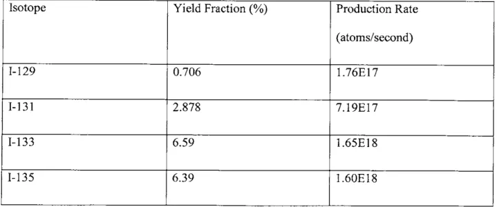
Table 2.1. Production rate and yield fraction of Cs and I fission products [51

Isotope Yield Fraction (%) Production Rate

(atoms/second)

1-129 0.706 1.76E17

1-131 2.878 7.19E17

1-133 6.59 1.65E18

The production rates are only part of the solution though, since these isotopes are all unstable. This means that as they build up as fission products, they will also be decaying away. Depending on the half-life of the radionuclide, eventually an equilibrium value may be reached during reactor operation where the production rate and decay rates are equal. This is described by the following first order, linear, non-homogenous differential equation:

dn X

dt - * n 2

Where p is the production rate, k is the decay constant (ln(2)/half-life), and n is the concentration as a function of time. Solving this differential equation involves finding a homogenous solution:

dnh _n ₂

= -n* 2

dt

nh = A * e-k*t 2

And a non-homogenous solution:

=

p

To get the final solution the homogenous and non-homogenous solution are added together and an initial value (n(O) = 0) is used to solve for the constant (A):

n(t) = A * e-k*t + Cs-134 1.121E-5 3.02E12 Cs-137 6.221 1.55E18 .2 .3 .4 .5 2.6

n(O) =A+( A = { n(t) = E (1 -e-t) 2.7 2.8 2.9

This solution shows how the concentration of a fission product will grow with time, and how an equilibrium value of p/X will be reached eventually. The time it takes to get to this equilibrium value will change based on the half-life of each isotope. After roughly 3/k seconds the

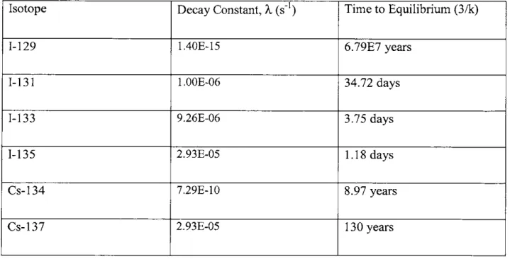
concentration will be at 95% of its equilibrium value. Table 2.2 lists the isotopes and the time it takes each to reach equilibrium:

Table 2.2. Decay constant and time to equilibrium of Cs and I fission products [61 Isotope Decay Constant, k (s-1) Time to Equilibrium (3/k)

1-129 1.40E-15 6.79E7 years

1-131 1.OOE-06 34.72 days

1-133 9.26E-06 3.75 days

1-135 2.93E-05 1.18 days

Cs-134 7.29E-10 8.97 years

Cs-137 2.93E-05 130 years

As the chart shows, several of these isotopes will easily reach equilibrium during normal operation of the power plant (1-131, 1-133, 1-135), but the others will not. A normal irradiation

made that two years of operation have passed, and that the reactor has been operating

continuously such that 1-131 is in equilibrium (>34.72 days). This means that 1-131, 1-133, and 1-135 will be at their equilibrium concentration, while 1-129, Cs-134, and Cs-137 will not be. By plugging two years into the equation previously solved for a conservative estimate of the

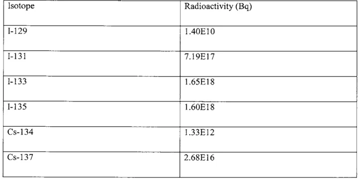
concentrations of the non-equilibrium isotopes can be found. Table 3.3 lists those quantities: Table 3.3. Total core inventories of Cs and I fission products

Isotope Radioactivity (Bq) 1-129 1.40E10 1-131 7.19E 17 1-133 1.65E18 1-135 1.60E18 Cs-134 1.33E12 Cs-137 2.68E16

When scaled for power these core inventories are consistent with known figures for larger nuclear power plants [7].

2.4 How much is released and in what form

To determine how much cesium and iodine are released in a containment vent first the chemical forms of each must be determined. Since Cs is an alkali metal and I is a halogen, they bond easily to form Cesium Iodide (CsI). As was shown in the previous section there is

in an accident situation where fission products are released from the fuel into the reactor vessel4_.

Since this percentage is so high for the purposes of this analysis we will assume that all Iodine in the core will be in the form of CsI. Taking the numbers above there will be 6.43E24 molecules

of CsI in the core at the time of the accident. This leaves about 90% of the core cesium which will overwhelmingly react with steam to form cesium hydroxide (CsOH) [8]. Again from the numbers above the remaining cesium equates to 4.12E25 molecules of CsOH.

Once the core inventories are established, it can then be determined how much of each isotope will escape in the venting. To get this data, we consult the source term for the reactor. The source term is determined by the regulator and reactor vendor through analysis of the various postulated beyond-design-basis accidents, taking into consideration also the plant design features (especially the containment features) that mitigate the consequences of those accidents. For this analysis the AP 1000 source term was used. The AP 100 is a similar design to the WSMR since it is a PWR with passive safety systems and in-vessel retention strategy for management of severe accidents [9].

In the AP 1000's source term document there are several different release categories which represent different ways radiation can be released to the environment. These categories are based on the various ways radiation can escape containment and enter the environment. For the purposes of this analysis it is assumed that there has been a severe accident leading to core meltdown, followed by a loss of containment cooling. This will lead to an increase in the

temperature and pressure inside containment eventually requiring venting before the containment fails. It is also assumed that this process will take longer than 24 hours from the initiating event. The release category which falls most in line with this scenario would be the containment

containment more than 24 hours post accident. In the AP 1000 document9 _{this type of accident}

has a calculated frequency of zero occurrences per reactor year, so unfortunately a source term was not provided. Without the necessary data to use the containment venting release, an alternative was used. The late containment failure release category is the most similar, it describes a situation where containment fails 24 hours post accident, so it was used.

In a late containment failure release the release fraction for cesium and iodine are: 1.2E-5 (0.0012%) for CsI and 1.1E-5 (0.0011%) for CsOH9. These numbers lead to 7.72E19 molecules (0.00013 moles) of CsI and 4.54E20 molecules (0.00075 moles) of CsOH being released with the vent. This amounts to a radioactivity concentration of 3.30E9 Bq/cm3

.

2.5 Hydrogen Production

The cladding which provides structural support and protection for the fuel and keeps fission products from escaping the fuel pin is made from a zirconium alloy, commercially known as zircaloy. Zircaloy has several properties which make it a good material for use in cladding specifically: low cross sections for neutron absorption, relatively high thermal conductivity and melting point. There is one significant drawback to using zircaloy as a cladding material; zirconium (zircaloy is over 97% zirconium) reacts exothermically with steam at high temperatures. The chemical equation for this reaction is:

Zr + 2H20 -+ Zr02 + 2H2 2.10

During normal operation this is not an issue because this reaction takes place slowly at normal reactor temperatures; however at the reaction rate is much higher at very high temperatures

(~1 0000C) [10], temperatures that can be reached in accident scenarios. The hydrogen gas produced in this reaction can be explosive if mixed in certain concentrations with oxygen from

containment air. This leads too many small LWR containments (especially BWR containments) being filled with inert nitrogen gas to prevent ignition of the hydrogen gas. However, if the containment is over pressurized and fails, hydrogen will escape and can explode. This led to the explosions in the Fukushima-Daiichi power plants.

In addition to being an explosion hazard this hydrogen will increase the pressure in containment, and will be a significant part of the release. Therefore the quantity of hydrogen produced is important for this analysis. The first step in finding the amount of hydrogen gas produced is to determine how much zircaloy is in the core. The fuel pins of the WSMR core are

9.5 mm in diameter with a cladding that is 0.572 mm thick, and are 2.4 m long, and a WSMR

core has 23,496 of these pins. With this data the total zircaloy volume can be found:

'0.0095 m'\2 (0.0095 m 23

IT * .0

)

From here using the density of zircaloy (6560 kg/m3), the percentage by weight of zirconium in zircaloy (98%), and the atomic mass of zirconium (91.227) the molar quantity of zirconium can be found:

0.904 m3*6560 g*1000 *0.98

M9 g -g 63705 mol Zr 2.12

91.227 mol Zr

The reaction shown above shows that for every mole of zirconium which reacts with the water there are two moles of hydrogen produced. In this analysis the assumption is being made that all of the core's inventory of zirconium is oxidized. This leads to 127,410 moles of hydrogen gas being produced in an accident scenario.

The reactor containment is essentially a large pressure vessel designed to contain fission products and gasses in an accident scenario. As a pressure vessel it falls under the American Society for Mechanical Engineer's boiler and pressure vessel code. This code determines safe limits for a number of factors relating to pressure vessels, specifically their design pressure. The limit on the design pressure is typically set to 2/3 of the actual max pressure the vessel can handle before failing [11]. The containment for the WSMR is designed to withstand pressures up to 250 psi (1.7 MPa). This means that the actual max pressure the containment can withstand is around 375 psi (2.59 MPa). When a containment is vented, radioactivity is released into the environment. In many cases this can lead to significant exposure for the population near the plant. Because the consequences of venting can be so serious, it is in everyone's best interests to not vent until absolutely necessary. This means that venting will occur when pressure inside the containment reaches the max pressure of 375 psi, and will continue until the containment

pressure is back to the design pressure of 250 psi. With these parameters venting prevents catastrophic failure of the containment, which would result in a much greater release. 2.7 Partial Pressures of H2 and Steam at maximum pressure

As mentioned previously the core will vent when pressure inside containment reaches 375 psi. The first step in categorizing what is released is to determine the composition of gasses in the containment before the release. There are three relevant materials inside the containment at this point: hydrogen gas, steam, and liquid water (the Westinghouse SMR uses a vacuumed containment so there are no other gasses). The amount of hydrogen gas is determined by zirconium oxidation and 127,410 moles of hydrogen gas are present if all zirconium in the core is oxidized. With this data the conditions of containment immediately before venting can be found.

A complete system of equations which will be used to solve for the initial conditions of containment. This set of equations includes the sum of partial pressures, the sum of liquid and gaseous volumes, and volume percentage of gasses (void fraction). The process for finding this solution is outlined in Appendix A, and the results are shown in Table 2.4.

Table 2.4. Containment data before vent

2.8 Vent Process

Once the conditions inside the containment are known modeling the vent itself can begin. The basic process for modeling the vent will take two steps repeated until the vent is complete. First the initial conditions will be used to find vent flow rates from a steam/gas critical flow model. Then with these flow rates known a small time step where this flow rate will be

considered constant will be looked at, and the conditions inside containment after this time step will be updated. Then these new conditions will be put back into the flow rate model, and so on. With small enough time steps this method is sufficiently accurate if computationally expensive. 2.9 Critical Flow Rate Model

The first step in this process is to find the flow rates of the steam and hydrogen being vented from containment. Compressible fluids being released from a volume of high pressure to one of a lower pressure undergo a phenomena known as critical flow. When solved for

mathematically the flow rate (or velocity or mass flux) from the high pressure region to the low

Containment temperature 212 C

Steam quality 0.0459

pressure one will be shaped like a parabola when the low pressure (back pressure, Pb) is varied such as in figure 4. 4000 3500 - 3000-2500 L 2000 1500 1000 5001II 0 0.5 1 15 2 25 3

Back Pressure (Pa) x 106

Figure 2.4. Mass flux with varying back pressure when solved mathematically The pressure where the mass flux peaks is referred to as the critical back pressure (Pcr). These results are only theoretical though, experimentally it can be shown that the mass flux will not decrease from the maximum value at back pressures less than Pcr. This disagreement between theory and experiment is due to the information that the back pressure is less than Pcr not being able to travel fast enough to be seen by the high pressure volume. At the peak flow rate the fluid is moving at the speed of sound in the fluid, which is the same speed which pressure waves move. This high venting speed prevents the effect of the lower back pressure from being perceived upstream, and keep the flow rate at its maximum value [12].

In the case of just an ideal gas or two phase mixture being the fluid vented the model of critical flow is fairly straightforward. However for a vent of an OFNP containment there is a mixture of these two types of fluids. Due to the more complicated nature of this system a new

model was put together to calculate the critical flow rates. This model is based on a complete set of equations solved numerically, and is explained in detail in appendix B. In general though it contains equations for the second law of thermodynamics, the sum of partial pressures, the conservation of energy (1s' law), a steam/water slip model, and an equation relating the mass percentage of hydrogen inside the containment to the densities of steam and hydrogen and the steam quality. This set of equations allows for us to solve for the speed and temperature at which the water and hydrogen is released, which are used to calculate a mass flux.

2.10 Containment Conditions after Timestep

With the critical flow model and a starting point another model to show the changes inside containment during the timestep must be found. This model will take in as inputs the starting conditions inside containment and flow rates from the critical flow models, and will then output a new set of conditions which will be used as to find the flow rate for the next timestep and as the starting conditions for the next timestep. This is again a complete set of equation solved numerically. The equations include the conservation of mass, conservation of energy, sum of the volumes of steam and water equaling the total volume, and the sum of the partial pressures. This model is explained in appendix C.

2.11 Vent

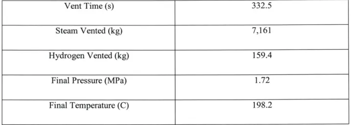
With the previous models completed the vent itself can now be modeled. Timesteps of 0.25 seconds were used to maximize accuracy without the process being too computationally expensive. Table 2.5 shows some of the results of this process.

Vent Time (s) 332.5

Steam Vented (kg) 7,161

Hydrogen Vented (kg) 159.4

Final Pressure (MPa) 1.72

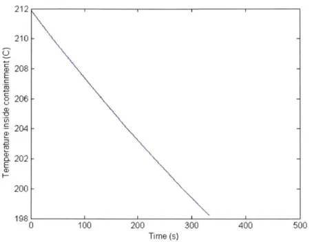
Final Temperature (C) 198.2

Figures 2.5-2.9 show how various parameters change throughout the vent process.

x106

100 200 300 400

Time (s)

Figure 2.5. Change in pressure inside containment throughout the vent 2.4 a) 2.3 E S2.2 a) S2 M, En 1.8 1.7 0 500 2.6 2.5

100 200 300 400

Time (s)

Figure 2.6. Temperature change inside containment during vent

100 200 300 400

Time (s)

Figure 2.7. Total mass of water inside containment during vent

212 210 208 206 204 202 200 CD CD CD C 198 0 500 1.85 1 1 .84 .83 .82 .81 1.8 .79 78 E 0 U _0 () (n 1 1.77 0 500 1

LO U) E E a) 26 25 24 23 22 21 20 19 18 0 100 200 300 400 500 Time (s)

Figure 2.8. Mass flow rate of vented water throughout vent

0.9 0.8 -0.7 2 0.6 E 0.5 0) 0 S0.4 0.3 0.2 0 100 200 300 400 500 Time (s)

As is to be expected the flow rates drop throughout the process as the pressure inside of

containment falls, but the flow rate of hydrogen falls by a much larger factor. This is due to the liquid water present inside containment at the beginning of this process. As the vent proceeds some of this liquid water will flash to steam, keeping the partial pressure of steam higher

throughout the vent process. This prevents the steam mass flow rate from dropping too rapidly. Additionally the curves all flatten out towards the end, which is a function of the reduced flow rates at lower containment pressures.

3 Fission Product Transport to Shore 3.1 Process of Fission Product Spread

\1

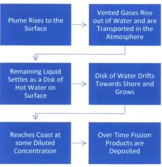
Figure 3.1. Process of Fission Product Spread

Following a vent of radioactive material there is a multistep process which describes how that material will be transported which is outlined in figure 3.1. First an estimation of how the vented material will rise to the surface of the ocean will be analyzed. As the material rises to the

form a disk-shaped patch of contaminated water on the surface of the ocean. This is called the near field part of the calculation. At this point all the gasses which were contained in the vent will rise out of the ocean and into the atmosphere. This includes the hydrogen gas, which is not radioactive and does not need to be modeled, and gaseous fission products, which are radioactive and whose spread needs to be modeled. The remaining disk shaped patch of contaminated water will drift with the local currents (possibly towards shore). Over time this patch will grow

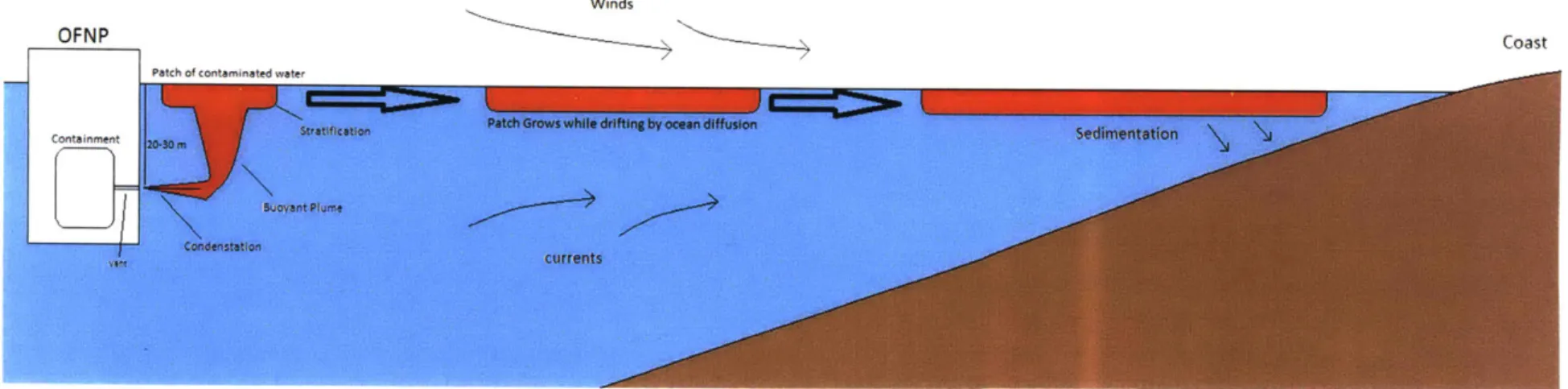
diluting the fission products it contains even more. Eventually this patch may reach shore with a lower concentration of fission products than when it was first formed. The process of the patch drifting and growing is referred to as the far field part of the calculation. Finally there will be deposition of fission products (predominately the longer lived cesium- 137) in the sediments onshore over time. This entire process is shown visually in figure 3.2.

5-12 NM

Winds

Coast

Patch Grows while

Stratification drifting by ocean diffusion

-

currents

Figure 3.2. OFNP venting process

OFNP

Patch of contaminated w

Containment 20,3 m

3.2 Assumptions for the near field calculation

Before beginning the near field calculation, some major assumptions need to be made and justified. First is that the steam which is vented out of containment quickly condenses before traveling any appreciable distance, and it can be treated as a hot water source for the purposes of buoyancy calculations. Venting steam into a stagnant body of cold water is referred to as direct contact condensation. This phenomenon is relevant in several other situations, and has been well researched. One such situation is inside a boiling water reactor (BWR) during a transient

overpressure or during a loss of coolant accident steam from the reactor pressure vessel is

directed into a suppression pool to prevent it from pressurizing the containment. The first step in determining how far the steam will travel before condensing is to find which condensation regime is applicable to this situation. Figure 3.3 shows a graph which distinguishes between the different regimes based upon mass flux (G), subcooling in the stagnant fluid (Ts-Tw), and the diameter of the vent pipe (D).

go 3D Condensation room* dagram for DCC 80 70 Ch mhg Coical jetting 60 -.50 40 EIpokdsI Jttng InterfacIaI condrsdibn osciletlon 20 - Diverpgnt jefi ng 10 0.04 No condensation 0.02 D [m] 0 500 1000 1500 Go [kg/rmns]

Figure 3.3. 3D Condensation regime diagram for direct contact condensation [131 The saturation temperature of water at the pressure the vent will be released into is between 133 C and 143 C depending on the depth of the vent. The stagnant temperature of the ocean at that depth can vary with respect to location, season, and current weather, but 20 C is used as a rough estimate. This leads to about 110-120 degrees of subcooling for an OFNP vent. The mass flux of steam coming out from the vent is roughly 3900 kg/m2_{s, and the current analysis was done}

with a pipe of 0.1 m diameter. Unfortunately these values are off the chart; however, it is clear that the situation of interest will fall into one of the jetting regions. This type of steam jet is shown in figure 3.4.

Turbulent jet

induced by a

condensing steam jet

Figure 3.4. Steam jet condensing in a pool of cold water [14]

This leads to being able to use a jetting correlation of which there are several. The experiments which form the basis for these correlations also do not go up to the mass fluxes seen in an OFNP vent, but can still be used to get a rough estimate. The correlations used are shown in Eq 3.1

[15] and 3.2 [16] X = 5923B-0_.6 6 _{G)o 0.3444 3.1} \Gm) X = 0.51B 0 . 7 _{(G 0.47 3.2}

In these equations Go and Gm are the mass flux the steam is being vented at, and the mean mass flux in the steam jet, respectively. Gm is estimated to be the critical vapor mass flux at the pressure of the seawater (732 kg/m2_{s). Also X refers to a normalized length of the steam jet and}

B is the dimensionless driving potential for the condensation process. Both are defined in Eq 3.3 and 3.4:

.~~1

B = c(rS-roo) 3.3

Ilfg

X = L 3.4

D

where C is the specific heat capacity of the water, T, is the saturation temperature of the steam, T, is the temperature of the seawater, hfg is the heat of vaporization of the steam, L is the length of the steam jet, and D is the diameter of the outlet pipe. Using the appropriate values (G0 =

3905 kg/M2s; T, = 133 C; T. = 20 C; and D = 0.1 m) leads to steam jet lengths of 26.9 cm and 32.8 cm from each correlation respectively. Since the vent will occur at a depth of between 20-30 m, this distance is clearly negligible. Additionally the outlet pipe can be shrunk to make this steam jet penetration distance even smaller. These correlations are not a perfect fit for the scenario of an OFNP vent, but their results do show that for any buoyancy calculation it can be assumed that all the steam condenses shortly after exiting the vent nozzle.

The second major assumption which needs to be justified is that this system can be treated as a simple plume. A situation where one fluid is injected into another can be classified in one of three groups: a jet, a plume, or a forced plume/buoyant jet. A jet is when the fluid comes out with significant momentum but is the same density as the surrounding fluid so has no buoyancy. A plume is the opposite where there is no significant momentum coming out, but there is

buoyancy due to a density difference. Finally a forced plume is a combination of the two where a fluid with significant momentum is forced out and has buoyancy. An OFNP vent is clearly a forced plume since it is injecting a mixture of hot water and hydrogen gas, which will be less dense than the surrounding seawater, but it is also injecting them with a large amount of momentum. However, at a significant distance from the source the momentum has diffused

plume can be used to describe its behavior [17]. An example of an underwater jet is shown in figure 3.5 and a plume is shown in figure 3.6.

Figure 3.5. Underwater Jet

In the case of an OFNP vent, the vent pipe will be placed parallel to the bottom of the ocean (sideways out of the platform), and therefore the direction in which the jet is released is perpendicular to the direction it will travel as a plume. This negates any significant effect

momentum would have, and therefore the simple plume model can be used. Since the material is being released horizontally one additional assumption must be made. In a horizontal release it would be possible for the bubbles of hydrogen gas to separate from the hot water and rise

separately. This would complicate the calculation, and it is assumed that the bubbles and water rise together.

The simple plume model depends on the kinematic buoyancy flux (B, which differs from the dimensionless driving potential from the previous calculation) which is the defined as [17]:

B = g ZQAPi 3.5

P

Since there are multiple different materials (hydrogen and a steam water mixture) which are being vented the total buoyancy flux is a summation of the fluxes for each material. In the buoyancy flux calculation g is acceleration due to gravity,

Q'

vented material, Api is the density difference between the surrounding fluid and the vented fluid, and p is the density of the surrounding fluid.

The assumption has been made that the steam condenses so quickly that its buoyancy can be ignored during the condensation process and it can be treated as saturated water coming out of the vent pipe. First the volumetric flow rates for both water and hydrogen must be calculated. This is done by taking mass flow rates found in the previous section and dividing them by the density of the vented material:

For the density difference ratios, the ratio for hot water to cold seawater can easily be calculated knowing each density (931.43 kg/m3 _{for hot water, and 1025 kg/M}3 _{for seawater):}

1025-g -931.43 kg

S M3 3 =0.091 _3.7

P 1025 k

The density of hydrogen is several orders of magnitude smaller than that of seawater, so it can be treated as roughly zero for this calculation. The density difference ratio with zero as the hydrogen density comes out to roughly 1 as shown below:

kg kg

1025 k0

m-P 1025kg3

in

3

This leads to the buoyancy fluxes shown in Table 1 for the input range from the previous study. Table 3.1. Buoyancy Flux of Simple Plume

Mass flow rate Water (kg/s) Mass flow rate H2 (kg/s) Buoyancy Flux (m4/s3)

23.0 0.117 12.57

38.3 0.266 28.57

Several other minor assumptions need to be made: first the final disk shaped patch of warm water and fission products which rises to the surface will have a depth of about 0.11 times the depth it was vented at for a plume originating from a point source [19]. At this height above the release point the concentration of any contaminants reaches a value within 10% of its ultimate value, and will be the depth of the contaminated water as it spreads horizontally. Second, the duration of the vent will be considered long when compared to the time it takes for the

release will be estimated to come from a point source (an acceptable assumption since the vent pipe is small). Finally, since the depth of the vent is only about 20-30 m horizontal currents in the ocean will not spread the contaminated water, and it will rise directly up to the surface. With these assumptions a simple plume model can be used to estimate the behavior of the vented material as it rises to the surface.

3.3 Near Field Calculation

The plume model used in the near-field calculation will allow for finding both the concentration of fission products once the vented material rises to the surface, and the size of that eventual mass on the surface of the ocean. From this a concentration of fission products and therefore a dose rate to any human or animal life can be calculated. Since the OFNP is sited well offshore, and there will be security zones surrounding the plant there should be no humans exposed at this point, but animal life could definitely be affected. The size of the disk of vented material and entrained water which eventually settles on the surface then becomes the input to the far field calculation which will look at ocean diffusion, to evaluate how this mass drifts with the currents while being diluted even further.

As a plume rises to the surface, it will entrain surrounding water diluting any contaminants it carries. This entrainment will cool the vented material while heating the entrained water until it eventually rises to the surface and sits there as a disk-shaped volume of contaminated water which is warmer than the water surrounding it. Figure 3.7 shows a diagram of this process.

H

* Buoyant plume

Transition

Horizontal spreading

xn

Figure 3.7. A plume rising to and spreading out at the surface [191

Since the depth of this disk shaped volume, h, is assumed to be 0.11 times the depth of the vent pipe, H, to find the concentration of contaminants and the size of the disk volume one has to calculate the amount of water entrained. The first step in the process of solving for the volume of entrained water is to find the buoyancy flux of the vented material (already found in the momentum length calculation). Once the buoyancy flux is known, the next step is to calculate the maximum time averaged vertical velocity on the axis of the plume (uc). The vertical velocity in the plume will be a Gaussian distribution peaking in the middle at a value of uc. This velocity will be a function of the buoyancy flux (B), the height from the plum origin (z), and the viscosity of the fluid (p). This can be simplified to exclude viscosity if the flow is fully turbulent, which will occur as the distance from the source increases. Eventually at a distance far enough away from the source equation 9 can be used to calculate u, [17]:

UC = 4.7B 3.9

Z3

where B is the buoyancy flux and z is the height within the plume from the source. With this velocity the volumetric flow rate at any point in the plume (Q) can be calculated from the equation [17]:

Q (z) = 7ruc (0.1z) 2 3.10

This equation multiplies the velocity found above with an area to come up with the volume flux. The area used is a circle of radius 0.1 *z. This both accounts for the widening of the plume as it rises, and allows for the use of the maximum time averaged velocity to be used to find the volumetric flow rate. With the volumetric flow rate at any point in the plume known the volume of the eventual patch of contaminated water can be found. From the assumptions the bottom of the disk is at:

z = H - h 3.11

where H is the depth from which the vent occurred and h is the depth of the final disk volume (H*0. 11). Then the volumetric flow rate at the bottom of the disk can be evaluated, and multiplied by the time which the vent takes to find the total volume of water which enters the disk [17]:

V=

Q

where V is the volume of the disk,

Q

V_ h U-

=-Table 3.2 summarizes these calculations for the range of inputs.

Table 3.2. Data from Near Field Calculation

3.13

Vented steam flow rate (kg/s) 23 38.3

Vented H2 flow rate (kg/s) 0.117 0.226

B (m4_/s3_{) 12.5 28.5} u, (m/s) 4.17 5.48 Vent time (s) 206 90 H (m) 20 30 h (m) 2 3 H-h (m) 18 27 Q(H-h) (m3/s) 42.4 125.5 V (m) 8744 11300 Radius (m) 37.3 34.6

uc is the maximum velocity at any horizontal cross section of the plume (will occur at the center). These values were calculated using equation 9, and are evaluated at H-h (the bottom of the contaminated patch of water).

The far field calculation will need to determine how fast the volume of contaminated water will drift towards shore, and how much it will grow as it does. Figure 3.8 shows how material (oil in the picture) sitting on the surface of the ocean will begin to spread from ocean diffusion.

Figure 3.8. Diffusion of Oil in the Ocean [201

The first part of this calculation depends greatly on currents offshore, which vary considerably based on time, season, and location. In many places the prevailing currents would actually push the contaminants further from shore and human population, leading to no contamination at the coast. Others may force the contaminated water to drift towards shore at various net speeds. A situation could even be imagined where a storm is coming in towards shore right as the vent occurs, and it pushes the contamination very quickly to the coast. For this analysis a

First looking at normal tidal currents shows that it is not trivial to determine how long it will take for the contaminated water to drift towards shore. Most tidal currents operate on a roughly 12-hour cycle, where the current speed can be modeled as a sine function fitting equation 3.14 [21]

v(t) = A + Bsin(2 * 7r * 12 hr) 3.14

This equation clearly shows that the current speed will oscillate as it moves. However, when looked at over several tidal periods an average speed can be found. In this case 0.318 kt (0.16 m/s) is used as a fairly conservative estimate of a normal offshore current.

The speed with which the water would move in the case of a storm helping to push it towards shore is less straightforward. Due to the highly unlikely nature of a storm arriving exactly when the vent occurs, a rough estimate will be made without significant study. Storm surge speeds of up to 15 mph (13 kt) have been observed in the past, and that will be used as the worst case current speed.

With the net speed towards shore known, the total time necessary for the contaminated water to reach the shore can be calculated based upon the distance from the OFNP to the shore:

t = D 3.15

where D is the distance to shore in nautical miles and v is the speed in knots. This time is the last input necessary to make use of an ocean diffusion model.

The most important assumption which will be made with regards to ocean diffusion is that there will be no vertical diffusion. The depth which the patch of contaminated water has immediately following the vent will not change as it travels and grows in the radial direction. This

estimate of the radioactivity that will reach shore. Another assumption has to do with the shape of the patch of contaminated water. It will clearly not stay in the shape of a perfect circle, likely it will begin to look like an amorphous blob over time. This blob will however, have an average radius which can be used to find an accurate estimate of its volume. The growth of this average radius is what will be tracked by the model of ocean diffusion. Finally it will be assumed that there will be no deposition of fission products on the ocean floor during the contaminated

water's transit towards shore. The only loss of fission products during this process will be by the radioactive decay of iodine over the transit time (cesium is too long lived to decay appreciably over these timescales).

Figure 3.9 shows the diagram which will be used to estimate the growth of the patch of contaminated water over time.

in'4. 2 (Cm 2) 101 1010 108 107 IC _{104 105} i(sec)

Figure 3.9. Okubo oceanic diffusion diagram [22]

This diagram was made using data from several experiments which tracked the size of a tracer put into the ocean in various parts of the world. It shows how the average radius of a patch of contaminated water will grow over time from only being a few meters across to tens of

kilometers. The only other input needed is a virtual time which represents the size of the patch

, , , 3 0 RHENO 1 964 3 t 23 0 1962 M NORTH SEA O 1962 H M 1961 I 0* 1 'M 02 _OFF A* 3 CAPE * #4 KENNEDY * e6

O NEW YORK BIGHT 0

* ob 0 # C OFF 0 d CALIFORNIA C- BANANA RIVER / ] MANOKIN RIVER 0 S : HOUR DI LY W EK TH 0 100 km I O km I km 100 m

once the plume has reached the surface (end of the near field calculation). This can easily be found using the equation from the diagram (with ar in cm, and t in seconds)[22]:

2' 0.011t2 3.16

Or rearranged:

t = 24 3.17

0.0 11)

Plugging in the radius found in the near field calculation into Eq 3.17 a virtual start time for the ocean diffusion process can be found. Then the final average radius can be found using Eq 3.16 with a time equal to the virtual start time plus the transit time calculated from Eq 3.17. The resulting radius can then be used to find the total volume of water in the patch with Eq 3.18:

V= 7rwrfh 3.18

Where h is the unchanged depth of the patch from the near field calculation.

Finally with the total volume of water in the patch, the concentration of the relevant fission products can be found. From previous work the total amounts of cesium and iodine released with the vent are known. The only variation in this comes from decay of iodine. That decay can be calculated by the following equation:

N, = Noe -*t 3.19

Where N1 is the final quantity of iodine present, N10 is the initial quantity of iodine present, X is

the decay constant for iodine 131, and t it the time it takes for the patch to travel to shore. Dividing the quantities of cesium and iodine by the previously calculated total volume the concentration can easily be found. The resulting data from this analysis is compiled in table 3

Table 3.3. Data from Far Field Calculation

Conservative analysis Best estimate analysis

Initial ar (m2) 37.3 34.6

Initial ar2

(M2) 1390 1200

Virtual start time (s) 7760 7280

Speed towards land (kt) 13 0.318

Distance to land (NM) 5 10 Transit Time (s) 1380 113000 Total time (s) 9140 120000 Final r (m) 45.2 923 Final ar2 (M2) 2040 853000 h (m) 2 3 Final volume (M3) 12800 8040000

Cs activity (Bq) 6.85E1 1 6.85E1 1

I activity (after travel, Bq) 7.84E12 7.06E12

Cs activity concentration 5.43E7 8.53E4

(Bq/m3

)

I activity concentration 6.15E8 8.79E5

3.5 Dose Rate to Humans

This concentration is important in the analysis, but it is not the final step in assessing the dangers to exposed human populations. For this a dose rate must be calculated. Activity only measures how many decays are happening per second; it says nothing about the type of radiation (alpha, beta, or gamma), how that radiation interacts with the human body, or the energy of that

radiation. Dose equivalent encompasses the amount of energy absorbed and the sensitivity of the various parts of the body to the radiation. There have been previous studies which relate

concentrations to dose rates via a coefficient for various methods of exposure [23]. Specifically external exposure when in contaminated water is relevant to this scenario. These coefficients are organized by body part with one all-encompassing effective dose. Multiplying this coefficient by the activity concentration (and some unit conversions) listed above, an effective dose rate can be found. These coefficients and the resulting dose rates are listed in table 3.4 below.

Table 3.4. Dose Rates at Shore

Conservative analysis Best Estimate analysis

Cs 137 Effective dose 1.49E-20 1.49E-20

coefficient (Sv/Bq s m3

)

1131 Effective dose 3.98E-17 3.98E-17

coefficient (Sv/Bq s m3

)

Cs 137 dose rate (mrem/hr) 2.86E-04 4.57E-07

1131 dose rate after 1 week 4.81 6.88E-3 (mrem/hr)

1131 dose rate after 1 month 6.60E-1 9.43E-4

(mrem/hr)

These rates compare to a limit of 2 mrem/hr for any unrestricted area, and a limit of 100 mrem in a year for members of the public [24]. In the best estimate analysis none of these limits would even be close to being reached, and the cesium dose rate in the conservative analysis is also far below the limit. However, in the conservative analysis the immediate dose rate due to iodine is higher than the 2 mrem/hr limit, but that will decay down to lower than that limit in less than three weeks even with no additional dilution by the ocean. Additionally as mentioned previously the conservative analysis relies greatly on the increased speed with which the contaminated patch will travel towards shore. The final volume of the conservative analysis is 600 times smaller than the best estimate, but if the same speed is used for both (everything else staying as is) this lessens to only 6.5 times smaller. Due to the significant sensitivity to current speed, it is likely that a more in depth analysis of currents will be done at any potential OFNP site. However, the current simplified analysis shows that doses to hypothetical swimmers, unaware of the potential radiation threat would be rather low and rapidly decay with time.

Moreover, if such an accident were to occur, the local population on shore would

immediately be warned and told to stay out of the water. Given the general public's fear of any radiation, it is highly likely that these warnings would be heeded and no humans would enter the contaminated water.

Of additional concern, not necessarily to humans, is the dose rate immediately after the vent settles on the surface of the ocean (after the near field). These numbers are listed in table 3.5.

Table 3.5. Concentration and dose rates following plume rising to surface

Conservative analysis Best Estimate analysis

Near Field volume (M3) 8744 11300

Cs137 activity (Bq) 6.85E1 1 6.85E1 1

1131 activity (Bq) 7.91E12 7.91E12

Cs activity concentration 7.83E7 6.06E7

(Bq/m3)

I activity concentration 9.05E8 7.0E8

(Bq/m3₎

Cs 137 dose rate (mrem/hr) 4.2E-4 3.25E-4

1131 dose rate (mrem/hr) 13.0 10.0

Again the cesium dose rates are small, and while the iodine dose rates are above NRC limits for human exposure they are still not very large. These doses could have an effect on life in the ocean which would be exposed to it, but it is unlikely to cause any major damage to the ecosystem.

4 Cesium Sedimentation

Following the transport of fission products to shore, a look at how these radioactive nuclides persist in sediments needs to be taken. Contaminants which stay in water will continue to be diluted by ocean diffusion over time, and as has been mentioned previously hopefully currents will push them towards open ocean. This cannot be counted on, however, and this chapter will look at in what quantities and how quickly fission products will be deposited into sediments.

Throughout this analysis of an OFNP accident and vent two major isotopes have been focused on as the most significant dangers to the public: Cesium 137 and Iodine 131. Iodine 131 is a fairly short lived isotope (half-life of roughly 8 days) and is not a major long term concern. Cesium 137 on the other hand is much longer lived (half-life of roughly 30 years), and is the primary danger after the first few weeks. When water carrying cesium comes into contact with sediments (most likely sand at the bottom of the ocean), some of the cesium will be

deposited onto the sediments. If this deposition occurs on a beach or some other area where humans are found, this could lead to these areas being quarantined. As the lack of an evacuation

zone following an accident is one of the major advantages of an OFNP over a terrestrial nuclear power plant, this is a significant concern.

4.2 Sediment-Water Exchange

In a sediment bed contaminates will be exchanged between the water and the sediments until an equilibrium is reached. This equilibrium is described by the partition coefficient (Kp) which is defined in equation 4.1 [25].

K = Cs 4.1

Where cs is the sorbed phase concentration at equilibrium (sorbed refers to contaminant in the sediment) and is defined as mass of contaminant per mass of sediment (g Cs/g sediment), and Cd

refers to dissolved phase concentration at equilibrium which is mass of contaminant per volume solvent (g Cs/l). This leaves K, with units of volume per mass. Given infinite time a sediment water mixture with a contaminant will reach the equilibrium defined by the Kp. There are a large number of factors which can affect Kp which makes it difficult to define exactly for any

situation, but based on tabulated data for cesium and sand like sediments a value of 28,600 ml/g was chosen [26].

While Kp defines the end point for this exchange the rate at which this equilibrium is reached is defined by the rate constant (K). The time rate of change for both the sorbed and dissolved concentrations are shown in equations 4.2 and 4.3 [26]:

d(pcd K*

(-

dt \Kp

d(pcs) = * (Cd - - _4.3

The density factor in the equation for the sorbed concentration is the density of the sediment in the solution and is calculated by using equation 4.4:

p = Ps * (1 - (0) 4.4

where ps is the density of the sediment, and p is the porosity of the sediment. These equations are intuitive in that the further away from equilibrium a system is the faster it will move towards that equilibrium. As with the partition coefficient there are a large number of factors which will affect the rate constant, and only through experiment in identical conditions can a true value be found. This is clearly beyond the scope of this thesis, so data from a previous study with similar

parameters to this scenario will be used here. From this data the value of 0.423 hr-' will be used as the rate coefficient [27].

As can easily be seen, equations 4.2 and 4.3 are equal in magnitude and opposite in sign to each other. This shows that the rate at which contaminant mass leaves the water is equal to the rate at which contaminant mass is adsorbed to the sediment (or vice versa), or in other words that the total contaminant mass is conserved throughout the process. This is an exchange of contaminant mass between the water column and the sediment, and there is no loss of

contaminants during the process. Clearly the cesium will radioactively decay over time, but on the timescales being looked at here that loss is insignificant due to the long half-life of cesium

137. There are also potentially losses through other mechanisms including cesium being absorbed by organic matter in the water, but those losses are also ignored for simplicity in the calculation.

4.3 System and Assumptions

This process of exchange between sediment and water will occur only once the

contaminated water comes in contact with sediments. As was mentioned in the previous section, vertical diffusion of the contaminated patch is ignored during transit from the platform to shore, so the depth of the patch does not change as it approaches shore. Due to this assumption the first time the cesium contaminated water will come into contact with the sand below it is when the patch reaches very shallow waters along the coast. Several simplifications have been made to the system to allow for an easier calculation. First is that once the contaminated patch reaches shore, it is assumed that the beach at that point is at a constant depth which is equal to the

thickness of the patch. This leads to a system where the contaminated water is sitting directly on top of the sand beneath it across the whole area of the patch.

The second assumption deals with the shape of the patch. Through ocean diffusion the patch will be shaped as a disk. Unfortunately this leads to complications when moving the patch along the shore so a square box shape with equal volume to the disk is assumed for ease of calculation.

Another major assumption is how far into the sediments the cesium contaminated water will travel. This is controlled by the diffusion coefficient of cesium in this system, and the length traveled can be calculated by using equation 4.5:

1 = 12 * D * t 4.5

Where D is the diffusion coefficient for cesium in sand (2E-4 cm 2s ) [28] and t is the time

elapsed. This equation will allow for the distance which the cesium will travel into the sediment given the time which it is present. For the case with a moving patch of water this distance will be calculated from the amount of time it takes for the entire patch to cross over a spot, and will then be assumed constant throughout the entire process. A cross sectional view of this system is shown in Figure 4.1.

--A