Discontinuous Space-Time Dependent Nodal
Method for Reactor Analysis
by
Chi H. Kang
Synthesis
B.S. in Nuclear Engineering
University of Maryland at College Park, May 1991 S.M. in Nuclear Engineering
Massachusetts Institute of Technology, June 1993 Submitted to the Department of Nuclear Engineering in partial fulfillment of the requirements for the degree of
DOCTOR OF SCIENCE at the
MASSACHUSETTS INSTITUTE OF TECHNOLOGY June 1996
Author
© Massachusetts Institute of Technology 1996. All rights reserved.
Department of Nucla EngiX~neering May 16, 1996
Certified by
Certified by
Professor Allan F. Henry Thesis Supervisor
,
_-Professor John E. Meyer Thesis Reader
Accepted by
C/
Chairman, Departmental
Protssor Jeffrey P. Friedberg Committee on Graduate Students
OF TECH-NOLOCCY
JUN 2 01996
Science
Discontinuous Space-Time Dependent Nodal Synthesis Method for Reactor Analysis
by
Chi H. Kang
Submitted to the Department of Nuclear Engineering on May 16, 1996, in partial fulfillment of the
requirements for the degree of DOCTOR OF SCIENCE
ABSTRACT
The accuracy and efficiency of a nodal synthesis method for steady-state and transient reactor analysis are investigated using DISCOVER (DIscontinuous Synthesis COde for VERification) computer code developed by the author. A three dimensional neutron flux shape of a reactor is approximated as a linear combination of predetermined two dimensional expansion functions. One dimensional mixing coefficients are computed using synthesis equations. The governing synthesis equations are derived by applying a variational principle. Discontinuous trial functions are allowed in both space and time. Two different approaches for updating Coarse Mesh Finite Difference (CMFD) discontinuity factors are incorporated in DISCOVER. One approach is a discontinuity factor synthesis scheme in which discontinuity factors are approximated as the weighted average of precomputed values. The other approach is a non-linear iteration scheme which forces the synthesis solution to match a quartic polynomial solution. Both flux and adjoint weight functions are edited from three dimensional steady-state CONQUEST calculations.
A few benchmark problems with and without feedback effects are tested using DISCOVER. For most cases, average nodal power errors are observed to be less than five percent of the reference solution, and eigenvalues are usually consistent up to three to four significant digits. In steady-state cases, there is about a five to tenfold reduction in computing time, compared with that of CONQUEST if the discontinuity factor synthesis scheme is applied. There is no reduction in execution time, however, if the non-linear iteration scheme is applied. This is attributed to the slow convergence rate of the synthesis solution method. In transient cases, even with the discontinuity factor synthesis scheme, the reduction in computing time is less than for steady-state cases. In fact, if the non-linear iteration scheme is applied, the execution time may even increase. The time-consuming matrix multiplication routine is the main cause of the increase in execution time. Still, a two to threefold reduction is possible if the discontinuity factor synthesis scheme is utilized. Also, real-time calculations are feasible for some slow transients.
Thesis Supervisor: Professor Allan F. Henry Thesis Reader: Professor John E. Meyer
ACKNOWLEDGMENTS
I would like to express my sincere gratitude to Professor Allan F. Henry, my thesis supervisor, for his guidance, encouragement and enduring patience. From the inception of the research idea to the completion of this thesis, he provided unending support and guidance and sometimes endured undue delays due to my incapability. It has been an honor and a pleasure to work with him throughout my years at Massachusetts Institute of Technology. I have nothing but a sincere admiration for his expertise and insights.
Thanks are also due to Professor John E. Meyer for his valuable advice on the incorporation of the thermal hydraulic model and for serving as my thesis reader. In addition, I would like to thank my friends at MIT for their friendship; Sangman for that somewhat disastrous fishing trip we took together for an elusive 2-foot-20-pound cod; Changhee for those occasional poker games; Changwoo for those drinking explorations through Boston bars. My stay at MIT was not only professionally enriching but also enjoyable because of their support and company.
Last, but not the least by any means, I owe my deepest gratitude to my wife, Seung, for her love and understanding. I would not be what I am without her unending encouragement and sacrifice. Thanks are also due to my parents and parent-in-laws for their love and support.
TABLE OF CONTENTS
A B ST R A C T ... 2
ACKNOWLEDGMENTS ... 3
LIST O F FIG U RES ... 7
LIST O F TA BLES ... 8 CHAPTER 1 INTRODUCTION ... 9 1.1 O verview ... ... 9 1.2 Background...11 1.3 Research Objectives...12 1.4 Thesis Contributions... ... 13 1.5 Thesis O rganization...14
CHAPTER 2 STEADY-STATE NODAL SYNTHESIS METHOD...15
2.1 Introduction ... 15
2.2 N odal Balance Equation ... 16
2.3 Finite Difference Nodal Coupling Equations ... ... 18
2.3.1 Boundary Conditions ... ... 21
2.3.2 Evaluation of CMFD Discontinuity Factors ... 22
2.4 Discontinuous Synthesis Equation ... 23
2.5 CMFD Discontinuity Factor Updating Schemes...27
2.5.1 CMFD Discontinuity Factor Synthesis Scheme...27
2.5.2 Non-Linear Iteration Schem e ... 28
2.5.2.a Transverse-Integration Procedure...28
2.5.2.b Polynom ial Expansion...29
2.5.2.c Weighted Residual Procedure...31
2.5.2.d Expansion Coefficient Solution...34
2.5.2.e Boundary Conditions ... 36
2.5.2.f Non-Linear Iteration Procedure...37
2.6 Sum m ary...39
CHAPTER 3 TRANSIENT NODAL SYNTHESIS METHOD...40
3.1 Introduction ... 40
3.2 Time-Dependent, Finite-Difference Nodal Equation...41
3.3 Discontinuous, Time-Dependent Synthesis Equation...43
3.4 CMFD Discontinuity Factor Updating Schemes...50
3.4.1 CMFD Discontinuity Factor Synthesis Scheme...51
3.4.2 Non-Linear Iteration Schem e ... 51
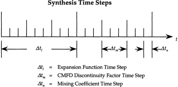
3.5 Time-Integration of the Synthesis Equation...53
3.6.1 WIGL Thermal Hydraulic Model...55
3.6.2 Cross Section Feedback... 56
3.7 Control Rod Cusping Correction...57
3.8 Sum m ary ... .. 58
CHAPTER 4 NUMERICAL SOLUTION METHODS ... 60
4.1 Introduction ... .... . . . ... 60
4.2 Steady-State Solution M ethods ... 61
4.2.1 N um erical Properties ... 61
4.2.2 CMFD Discontinuity Factor Iterations...62
4.2.3 O uter Iterations...63
4.2.4 LU Factorization... ...67
4.2.5 Steady-State Iteration Strategy ... 69
4.3 Transient Solution M ethods ... 70
4.3.1 N um erical Properties ... 71
4.3.2 Dynam ic Frequency Estim ation...72
4.3.3 Transient Solution Procedure ... 72
4.4 Sum m ary ... 73
CHAPTER 5 APPLICATION OF SYNTHESIS METHOD...75
5.1 Introduction ... .. ... 75
5.2 Prelude to Synthesis Results ... 76
5.2.1 Com puter Code ... 76
5.2.2 Transverse Leakage Approximations ... 77
5.2.3 Pow er Distribution Errors ... 77
5.2.4 Execution Times... ... 78
5.3 The Three-Dimensional LM W Reactor...79
5.3.1 The Three-Dimensional LMW Problem Without Feedback ... 79
5.3.2 The Three-Dimensional LMW Problem With Feedback...89
5.4 The PW R Operational Transient...94
5.5 The PWR Coolant Inlet Temperature Transient...100
5.6 Summ ary...103
CHAPTER 6 CONCLUSIONS AND RECOMMENDATIONS...105
6.1 Overview and Conclusions ... 105
6.2 Recom m endations for Future W ork...107
6.2.1 A Code Allowing Different Number of Expansion Functions A x ially ... 1 0 7 6.2.2 Further Investigation of Discontinuity Factor Updating P ro ced u res ... 10 8 6.2.3 Non-Iterative Discontinuity Factor Updating During Transient ... 108
6.2.4 A Quasi-Static Method Using Synthesis As Shape Update...108
R EFER EN C ES ... 110
APPENDIX A THE QUADRATIC TRANSVERSE LEAKAGE MOMENTS AND COEFFICIENTS ... 113
A.1 The Quadratic Transverse Leakage Approximation...114
A.2 LHS-Biased Quadratic Transverse Leakage Approximation...116
A.3 RHS-Biased Quadratic Transverse Leakage Approximation...117
A.4 Flat Transverse Leakage Approximation...119
APPENDIX B NUMERICAL STUDY OF THERMAL HYDRAULIC M O D ELS...120
APPENDIX C PROBLEM SPECIFICATIONS ... 126
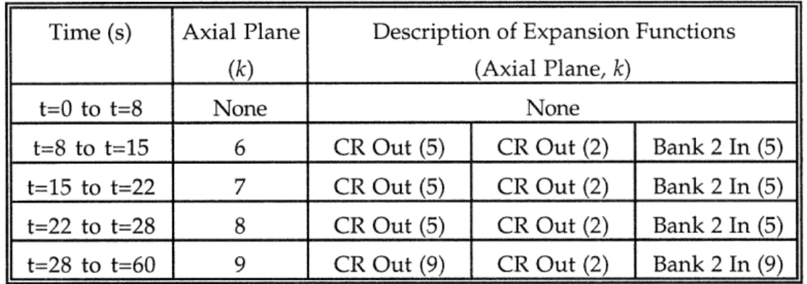
C.1 The LMW LW R Transient Problem ... 126
LIST OF FIGURES
Figure 2.1 Diagram indicating Interface and node labeling conventions ... 19
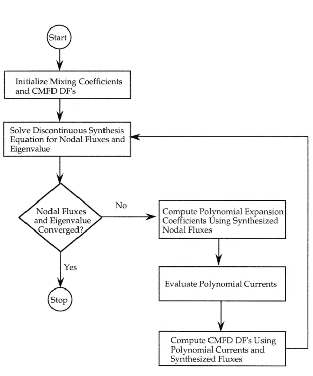
Figure 2.2 Non-linear iteration flow diagram...38
Figure 3.1 Diagram showing the subdivision of time steps in synthesis m eth od ... 55
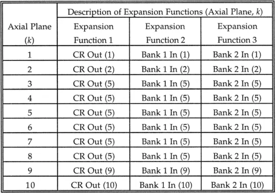
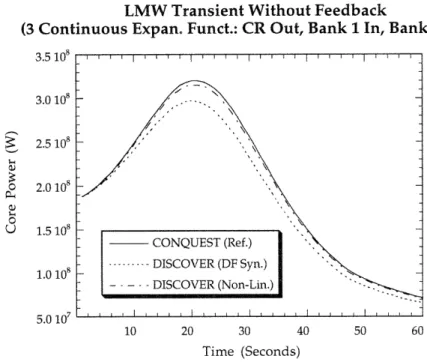
Figure 5.1 Core power vs. time for the LMW transient without feedback. (3 Cont. Expan. Functions: CR Out, Bank 1 In, Bank 2 In) ... 82
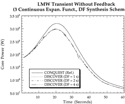
Figure 5.2 Core power vs. time for the LMW transient without feedback. (DF Synthesis Scheme with different time steps)...84
Figure 5.3 Core Power vs. time for the LMW transient without feedback. (Non-Linear Iteration Scheme with different time steps)...84
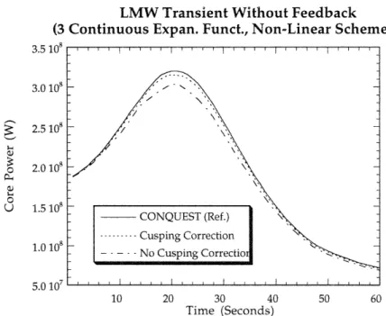
Figure 5.4 Core power vs. time for the LMW transient without feedback demonstrating the cusping correction ... 85
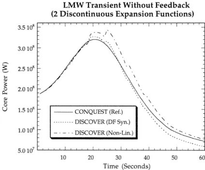
Figure 5.5 Core power vs. time for the LMW transient without feedback. (2 Discontinuous Expansion Functions)...87
Figure 5.6 Core power vs. time for the LMW transient without feedback. (3 Discontinuous Expansion Functions) ... 88
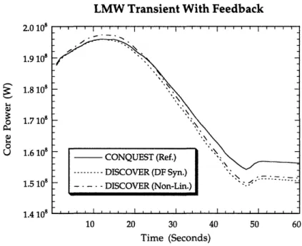
Figure 5.7 Core power vs. time for the LMW transient with feedback. ... 91
Figure 5.8 Core power vs. time for the LMW transient with feedback. (DF Synthesis Scheme with several different time steps)...92
Figure 5.9 Core power vs. time for the LMW transient with feedback. (Non-Linear Iteration Scheme with several different time steps) ... 93
Figure 5.10 Core power vs. time for the LMW transient with feedback demonstrating the effects of cusping correction ... 93
Figure 5.11 Core power vs. time for the PWR operational transient ... 96
Figure 5.12 Axial power shape for the PWR operational transient. (t = 0 s) ... 98
Figure 5.13 Axial power shape for the PWR operational transient. (t = 60 s)...98
Figure 5.14 Axial power shape for the PWR operational transient. (t = 120 s)...99
Figure 5.15 Core power vs. time for the LMW transient with feedback. (Control rod group 1 withdraw al) ... 100
Figure 5.16 Core power vs. time for the PWR coolant inlet temperature tran sien t...102
Figure B.1 Space-time discretization used for IDC model...121
Figure B.2 Space-time discretization used for WIGL model...121
Figure B.3 Two-node problem used to test thermal hydraulic models...123
Figure B.4 Average enthalpy vs. time steps for r = 0.1...123
Figure B.5 Average enthalpy vs. time steps for r = 0.5...124
Figure B.6 Average enthalpy vs. time steps for r = 1.0...124
LIST OF TABLES
Table 5.1 Convergence criteria used in DISCOVER and CONQUEST...79 Table 5.2 Expansion functions for the LMW steady-state problem without
feedback. (3 Expansion functions)...81 Table 5.3 A summary of the results for the LMW steady-state problem
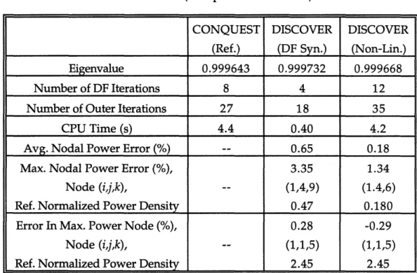
without feedback. (3 Expansion Functions)...81 Table 5.4 A comparison of errors for the LMW transient without feedback...82 Table 5.5 A summary of execution times for the LMW transient without
feedb ack ... 83 Table 5.6 Expansion functions for the LMW steady-state problem without
feedback. (2 Expansion Functions)...85 Table 5.7 A summary of the results for the LMW steady-state problem
without feedback. ( 2 Expansion Functions) ... 86 Table 5.8 Changes in expansion functions for the LMW transient
problem without feedback. (2 Expansion Functions)...87 Table 5.9 Changes in expansion function for the LMW transient
problem without feedback. (3 Expansion Functions)... 88 Table 5.10 Expansion functions for the LMW steady-state problem with
feedback. (All expansion functions generated at 184.8 MWth)...90 Table 5.11 A summary of the results for the LMW steady-state problem with
feedb ack ... 90 Table 5.12 A comparison of errors for the LMW transient with feedback ... 91 Table 5.13 A summary of execution times for the LMW transient with
feedb ack ... 92 Table 5.14 Expansion functions for the PWR steady-state and transient
problems. (All expansion functions generated at 667.6 MWth) ... 95 Table 5.15 A summary of the results for the PWR steady-state problem with
feedb ack ... 96 Table 5.16 A summary of execution times for the PWR operational transient...97 Table 5.17 Expansion functions for the PWR inlet coolant temperature
tran sien t ... 10 1 Table 5.18 A summary of the results for the PWR steady-state problem...102 Table 5.19 A summary of execution times for the PWR coolant inlet
CHAPTER 1
INTRODUCTION
1.1 Overview
One of the most fundamental quantities that pervades every aspect of nuclear reactor core design and operation is the neutron flux. Ever since the beginning of the nuclear era, great efforts by many bright minds have been devoted to answering the seemingly simple question of how neutrons are distributed in a reactor core. The difficulties in answering this question do not lie in lack of understanding of the physical phenomena or in inadequate modeling. The governing neutron balance equation, the Boltzmann Transport Equation, is well understood, and basic nuclear data are readily available. The problem stems from the enormous difficulties in solving the Boltzmann Transport Equation. It takes seven independent variables to describe the directional neutron flux. And, even with the super computers of today, it is a formidable task to carry all those variables in their discretized forms when a very accurate reference solution is mandated. It is impractical to solve the Boltzmann Transport Equation repeatedly for a particular reactor design or fuel loading optimization. Fortunately, for Light Water Reactors (LWR), in which high-order transport effects are negligible, it is also unnecessary.
Diffusion theory, which assumes a first order directional dependence of neutron flux, has been shown to be sufficient for LWR's. This diffusion theory approximation eases some of the difficulties associated with solving the Boltzmann Transport Equation, and has been the basis of design and safety calculations associated with LWR's. Yet, three dimensional spatial discretization of the neutron diffusion equation still retains the problem of having to calculate millions of fine-mesh neutron fluxes. Because of this limitation, most computer codes employing a fine-mesh representation of the neutron diffusion equation resort to either one- or two-dimensional analysis taking advantage of symmetry conditions.
Over the last twenty years, considerable research effort has been directed toward developing nodal diffusion theory, which allows a much more coarse spatial discretization (i.e., assembly size mesh). With the introduction of equivalence parameters (usually called discontinuity factors), which account for homogenization, discretization and even diffusion theory errors, the solution of the nodal diffusion equation can replicate a reference solution obtained by either a fine-mesh diffusion calculation or even a transport calculation. The nodal diffusion equation, therefore, reduces the number of spatial fluxes by orders of magnitude and makes three dimensional analysis feasible on desk-top computers.
The nodal theory greatly reduces the computing efforts associated with reactor analysis and, thereby, serves as an excellent tool for a nuclear analyst to optimize a particular reactor design or a fuel loading pattern without an undue burden of long waiting time between each computation. Furthermore, the realization of a real-time calculation, at least for some slow transients not requiring very small temporal steps, is within reach with adequate computers. The natural progression in research efforts, therefore, is to combine an efficient nodal code into an automatic controller to regulate steady-state and transient behavior of a nuclear reactor on a real-time basis. Accomplishing this ambitious goal, however, requires a further reduction in computing time without sacrificing the computational accuracy. This goal can be realized in part by faster computers, but it will also require further refinements in nodal theory and development of more efficient computer codes.
This thesis concentrates on the development of a nodal synthesis method which can be used for steady-state and transient reactor analysis. The primary goal is to reduce further the computing efforts without unduly compromising the accuracy of neutron flux determination.
1.2 Background
The synthesis method in reactor analysis approximates the neutron flux shape of interest as a linear combination of predetermined expansion functions (sometimes called trial functions). These expansion functions are, in fact, educated guesses of an actual neutron flux shape. Although, little theoretical justification exists for deciding which expansion functions to select, previous numerical studies [Y-1,Y-2,Y-3] indicate no significant problem in choosing expansion functions based on physical intuition and past experience. On the contrary, there is a firm theoretical ground for obtaining the mixing coefficients, the parameters which specify how given expansion functions should be combined to replicate the actual neutron flux shape as closely as possible. Both a weighted residual method and a variational principle are used to derive synthesis equations having mixing coefficients as the unknowns. The most attractive feature of the synthesis method stems from the fact that the number of mixing coefficients is orders of magnitude less than the number of discretized flux values. Thus, computational requirements can be greatly reduced with proper application of the scheme.
The synthesis method in reactor analysis was first applied to a fine-mesh representation of the neutron diffusion equation. Because of the enormous computational requirements associated with a fine-mesh discretization, the synthesis method was the only practical approach to calculate three-dimensional neutron fluxes. Earlier studies by Yasinsky and Kaplan [Y-1,Y-2,Y-3] showed that space-dependent synthesis employing discontinuous sets of axial and temporal expansion functions was capable of constructing accurate space-time neutron fluxes. Yet, no mention of computational speed was given in these studies. Furthermore, all the numerical tests were performed for either one- or two-dimensional reactors.
Recently, there have been several attempts to apply the synthesis method to the nodal diffusion equation. K. Lee studied a point synthesis method, which utilized three-dimensional expansion functions, based on an analytical nodal diffusion theory model [L-5]. The point synthesis model produced satisfactory results involving homogeneous changes in reactor conditions. However, because of the inherent limitation of using three-dimensional expansion functions, heterogeneous changes in reactor conditions (i.e., control rod motions) were not tested. Moreover, the computational speed did not improve relative to the reference QUANDRY [S-2] calculations.
W. Kuo investigated the point synthesis method based on a finite difference nodal diffusion theory [K-1]. He suggested a synthesis scheme to update the Coarse Mesh Finite Difference (CMFD) discontinuity factors. The results were encouraging as
far as accuracy was concerned, but the computational speed again was not satisfactory. He indicated the additional matrix multiplication steps needed in the synthesis method as the main cause of inefficiency. Moreover, his study was limited to one-dimensional reactors which would not exhibit the complexities associated with multi-dimensional analysis.
R. Jacqmin investigated a semi-experimental instrumented nodal synthesis method in which the synthesized neutron fluxes were force to match, in a least-squares sense, neutron detector readings [J-1]. It was semi-experimental in that the detector readings were generated by simulated transients rather than by actual experiments. Although there were some concerns about measurement noise, the number and positions of detectors, and detector characteristics, his study showed that nodal fluxes could be reconstructed in real-time with maximum errors of a few percent.
J. Hughes applied an instrumented nodal flux synthesis method to analysis of the Massachusetts Institute of Technology Reactor, MITR-II [H-1]. Detector measurements were collected using fission chambers placed around the core. The experimental results indicated that the instrumented synthesis accurately reflected the changes in reactor conditions in real-time, though they did not replicate the reference solutions with acceptable accuracy.
1.3
Research Objectives
The objective of this study is the development of an efficient (fast and accurate) discontinuous space-time dependent nodal synthesis method for the solution of the three-dimensional, few group, steady-state and transient neutron diffusion equations. No restriction is placed on the number of energy groups, and neutron upscattering is allowed. The synthesis method permits both spatially and temporally discontinuous flux expansion functions while maintaining initial adjoint weight functions. Although different flux expansion functions may be adopted at different axial planes and different time steps, their total number is kept constant. The CONQUEST code, developed by J. Gehin [G-1], is used to generate two-dimensional flux expansion functions and adjoint weight functions. A three-dimensional CONQUEST calculation rather than a series of two-dimensional calculations is performed for the generation of expansion functions.
Two different discontinuity factor updating approaches are incorporated to test their accuracy and speed. A non-linear iteration scheme, where finite difference nodal
fluxes are forced to match a quartic polynomial nodal solution, is one way to update CMFD discontinuity factors. This scheme is successfully implemented in the CONQUEST code, and results obtained from it indicate excellent accuracy [G-1]. However, one of the shortcomings of this non-linear iteration scheme is its computational burden: Preliminary analysis indicates that more than half of the total computing time is spent in updating CMFD discontinuity factors. This shows that if significant reduction in computing effort is to be realized, a more efficient updating scheme should be considered. A discontinuity factor synthesis scheme suggested by W. Kuo [K-1] is another approach. Though this scheme lacks the theoretical basis that the non-linear iteration scheme possesses, the results obtained are encouraging [K-1]. Furthermore, the discontinuity factor synthesis scheme requires much less computational efforts than the non-linear iteration scheme.
Direct inversion of matrices, rather than iterative inversion, is adopted in the synthesis solution procedure for two reasons. First, the number of unknowns are on the order of tens to hundreds and, thereby, makes the direct inversion practical. Second, the matrix to be inverted lacks the structure that guarantees that the iterative inversion techniques converges. A simultaneous group solution is adopted and the band structure is exploited in the direct inversion procedure.
Finally, a simple, one-dimensional thermal hydraulic WIGL model [V-1] is adopted to allow feedback effects. This model is selected for its simplicity and comparison purpose because the CONQUEST code adopts the same model.
1.4 Thesis Contributions
The space-time synthesis method was applied years ago to a fine-mesh representation of the neutron diffusion equation, but has not been previously attempted for a nodal method. Thus, the main contribution of this thesis is the development of a computer code which can serve as a tool to test the accuracy and efficiency of the discontinuous space-time nodal synthesis method. Another contribution is the identification of the numerical properties of the synthesis method and the subsequent development of numerical solution methods consistent with them. The implications of discontinuous usage of expansion functions are identified variationally. Also, an eigenvalue iteration strategy which maximizes the computational speed is tested for its effectiveness.
1.5 Thesis Organization
Chapter 2 presents the complete mathematical derivation of a steady-state nodal synthesis method. First, a finite difference method which incorporates CMFD discontinuity factors is developed. Then, a nodal synthesis method is derived by applying a variational principle to the finite difference nodal equation. Two different discontinuity factor updating approaches (a discontinuity factor synthesis scheme and a non-linear iteration scheme) are presented next. For the non-linear iteration scheme, a polynomial nodal method is discussed in great detail.
Chapter 3 offers a similar derivation of a transient nodal synthesis method. Although not implemented in this thesis, the implications of using a different number of expansion functions at different time steps and of allowing flux and adjoint expansion functions to change at the same time are discussed in light of the variational principle. The thermal hydraulic and cross section feedback models as well as a cusping correction
model are also presented.
Chapter 4 presents the numerical solution methods for the steady state and transient nodal synthesis method. The eigenvalue iteration procedure and the direct matrix inversion technique are discussed. Also, a temporal solution advancing strategy is presented.
In Chapter 5, the results from several steady state and transient benchmark problems with and without cross section feedback effects are presented.
Finally, Chapter 6 presents the summary and conclusion of this study. Some recommendations for future research are also made.
CHAPTER 2
STEADY-STATE
NODAL SYNTHESIS METHOD
2.1 Introduction
This chapter presents the derivation of a steady-state nodal synthesis equation from the few-group diffusion equations. First, the finite-difference nodal equation, which is mathematically rigorous with the introduction of CMFD discontinuity factors, is derived in Cartesian geometry. With appropriate CMFD discontinuity factors, the finite-difference nodal equation can reproduce any reference solution. Second, a discontinuous nodal synthesis equation is derived by applying a variational principle to the finite-difference nodal equation. Next, two different discontinuity factor updating schemes, a discontinuity factor synthesis scheme and a non-linear iteration scheme, are introduced. A polynomial nodal method, which produces accurate results even when assembly-size spatial discretization is employed, is discussed in great detail. The non-linear iteration scheme results when the synthesis solution is forced to match the polynomial nodal solution. Although it lacks the theoretical basis of the non-linear iteration scheme, the discontinuity factor synthesis scheme is introduced for its computational simplicity and efficiency.
2.2
Nodal Balance Equation
The derivation of the nodal balance equation starts from the few-group, steady-state diffusion equation in P1 form without an extraneous neutron source [H-2]
G
V Jg (r) + tg r)=
X[xgvfg,(r)
+ Egg,(r) gg,(r),
(2.1a) Jg(r) = -Dg(r)VOg(r) g = 1,2,...,G. (2.1b)Where
Jg (r) = neutron current for group g, Og(r) = scalar neutron flux for group g,
Zt (r) = macroscopic total cross section for group g,
I fg(r) = macroscopic fission cross section for group g,
gg. ,(r) = macroscopic scattering cross section from group g' to g,
Dg (r) = diffusion coefficient for group g,
ZXg = fission spectrum for group g,
A. = reactor eigenvalue,
v = mean number of neutron emitted per fission,
G = total number of energy groups.
It is a bit of a misnomer to call Eqs. (2.1a) and (2.1b) the few-group diffusion equation because the multi-group diffusion equation assumes the exact same form. The methods by which the group parameters (cross sections and diffusion coefficients) are obtained
distinguish one from the other. The few-group diffusion equation uses the neutron energy spectrum obtained by a separate calculation to determine the group parameters while the multi-group diffusion equations uses an arbitrarily assumed energy shape (i.e., Maxwellian distribution in the thermal range). Note that, according to this distinction, group parameters obtained by averaging over a detailed energy spectrum are "few-group constants" even though the number of groups may be hundreds. With the number of "few-groups" this large, however, the distinction is generally abandoned and the model is referred to as a multi-group scheme [H-2].
The few-group diffusion equation in its spatially discretized form has been the basis of most safety and fuel depletion calculations for LWR's, and many utilities still perform reactor analyses using computer codes adopting this scheme. The solution of the fine-mesh, few-group diffusion equation in its three-dimensional form, however,
requires an prohibitively large computing time. Thus, the repeated use of the fine-mesh diffusion equation is undesirable in fuel loading, depletion and reactor safety calculations which are inherently iterative in nature. This difficulty is somewhat alleviated by exploiting symmetry conditions and the axially homogenous geometry that exists in most LWR's, but even a two-dimensional analysis requires a formidable computing effort, and furthermore, some of the reactor systems do mandate three-dimensional analyses.
The nodal diffusion equation makes three-dimensional analyses feasible by employing much more coarse spatial discretizations (i.e., assembly-size nodes). However, it requires additional equivalence parameters, called discontinuity factors, to replicate the reference solutions obtained from either the Boltzmann Transport Equation or the fine-mesh diffusion equation. The physical meaning of discontinuity factors will be discussed in Section 2.3. In Cartesian geometry, Eqs. (2.1a) and (2.1b) are
dJjx(x,y,z)
+--J(x,y,z)
+ JgZ (x, y,z) +Z eg (x,y,z)Og(x,y,z)G (2.2a)
I
IXgVjg
(xyZ) +Z ,(x'y,z) Og' (xy,z),g=
Jgu(x,y,z) = -Dg(x,y,z) dg(x,y,z) u = x,y,z. (2.2b)
The node (i,j,k) and its widths are defined by
xE [x.,xj+1]
hx
-xj+ -x,Y [Yj'Yj+] he yj+2 - Yj, (2.3)
Z [zk,Zk+1] hk Zk+1 - Zk,
and the node volume is
Vijk - .hxhyih. (2.4)
The nodal balance equation is obtained by integrating Eq. (2.2a) over the volume of node (i,j,k) and then diving by Vilk
l[jk(x,+,)
J
(xi)]+ ;(y+) 'Ik + z k+1 JZk+
I hx' k yl 4(Zk+ ] +2.5J(Y ) z' (z+j]
G Xg Z(2.5)
+ -ri"
09111C V
4
"
+ -
V
j 1
"
1
1
where the node-averaged flux and the surface-averaged current are defined by
ijk • Vilk 1 Jx• dx,+l dy dxy Zk+l dz t(x, y, z), (2.6)
1 gz
Jmn
(U) -• 1 dv w ""dwJg,, (u,v,w), u-x,y,z, v u, w u,v. (2.7)J1gU) f yn w''V#U W#UV 27
The group parameters within node (i,j,k) are assumed to be constant.
Although derived without any approximation, Eq. (2.5) is not complete by itself because it contains both node-averaged fluxes and surface-averaged currents as the unknowns. Therefore, additional equations relating node-averaged fluxes and surface-averaged currents must be provided. These additional equations are called nodal
coupling equations and discussed in the following section.
2.3 Finite Difference Nodal Coupling Equations
The finite-difference nodal coupling equations are derived by integrating the second P1 equation, Eq. (2.2b), over a surface and diving by its widths
Jn
(u)= -D'"gd
nix(u), (2.8)gUg where the surface-averaged flux is defined by
'h(u)
=h
dv J
1dw (u,v,w),
(2.9)
V WV
and by approximating the spatial derivative as a simple first-order difference
-Itmn mn ('
Jmn l(u)=Dmn gu (2.10)
l/ (U) h /2 /D2 0)
where u' indicates the positive side of the interface shown in Figure 2.1. Similarly, the same surface-averaged current at the interface u, can be approximated for node 1-1
mn) g-1lmn
l' (u/) n h 2 /-D-,n , (2.11)
U1-1 Ul Ul+1
Figure 2.1: Diagram indicating Interface and node labeling conventions.
Eqs. (2.10) and (2.11) are incomplete because they are valid only when a very fine-mesh spacing is considered. When assembly-size nodes are used, which is the very goal of a nodal theory, a large error will result. The assumption of a linearly varying flux is more often than not invalid for assembly-size nodes.
This difficulty is overcome by the use of correction factors, first introduced by Smith [S-1], to force Eqs. (2.10) and (2.11) mathematically rigorous. The correction factors, f',mn and
flm,
for the opposite sides of the interface between node (1-1,m,n)and (l,m,n) are defined by
f1-1,mn_ _i (g Uj) f gu+ Ygu n ' (2.12) 4fm (U1) f"ii • imn U_ Igu )
where A'n,(u l) is the true surface-averaged flux. Examination of Eq. (2.12) shows that
the correction factors have the effect of making the surface-averaged flux discontinuous if f1j1n and iand are not identical. For this reason, the correction factors are called discontinuity factors [H-3]. Inserting the discontinuity factors given in Eq. (2.12) into Eqs. (2.10) and (2.11) results in the following equation
-lmn ni/)n ( )f Ini nu
Jmn U)- Imn O gu(U)19I
Jgu (ul) = -Dr"g m h7(u~/f'2
" hL/2
- -B-mmn-lmn (2.13)
l-l'- mn gu (U --gu+ Yg
= -D hul/2
When used with the reference values for the currents and fluxes, Eq. (2.13) also serves as the definition of the discontinuity factors.
Although the discontinuity factors are introduced as the correction factors intended to reduce the spatial discretization errors when a large node spacing is used, they also can be used to correct for cross section homogenization errors and diffusion theory approximation errors. These correction factors will be referred to as Coarse Mesh Finite Difference (CMFD) discontinuity factors throughout this thesis to distinguish them from another set of discontinuity factors introduced later in this chapter.
Now, the finite-difference nodal coupling equation, relating surface-averaged currents to node-averaged fluxes, is obtained by eliminating the surface-averaged fluxes in Eq. (2.13) using the continuity condition implied in Eq. (2.12)
h Im n I - 1
_ h'
fU2
h"j ____ 11rn"'mn gu- u gu- "Imn -,mn
(2.14)
Jgu (UI 2Dmn I - Im 2DI--Rmn n-Trg Vg (.
L
gu 2Dg1 rn f gu+ fSubstituting Eq. (2.14) and its equivalent coupling equation for the node surface ut+1 into Eq. (2.5) results in the following finite-difference nodal balance equation
r
11/
1 h'
fg
h _x- l_ f g-+1,k , k+~ i jk -o -1
h"
2Di'k ggx + i-l,sk2Di-1,]k
g fgx -+1 g JIfqk Il .+1 - fi]k
1 h
h gx+ -ik -_+lfkh'
2Dijk
z+ljk +2D
+,k +,jk g hx ggx - g fg9xI-' 1 hf;k
+h-1 ijk y g f;y+ g Igy+1
h]
ilkhi+'
i1
jk+
Y +_ + y Jk ,+,kh 2Dijk fi,j+l,k 2Dij+l,k ,+l,k g g
y g gy-
,g-y-1 hf
ff_
hki- - _ -_ k_,-h 2Dhk IIk- 2D. k -1 fitjk- (.g
11 h(
ff±
+
h__+__ fz qk ~q,k+2 (2.15)_____ - k
+h
k2D ik fVk+I2Di"'
I k+1yq,
k Yg= 1Z + J+gZ
z
k Ig
k I
gz-ijk--'ijk = 1)pij N~ jk---- i
First, note that only the ratios of the CMFD discontinuity factors appear in the final nodal balance equation. Second, if CMFD discontinuity factors are unity, Eq. (2.15) reduces to the mesh-centered, finite-difference diffusion equation.
Eq. (2.15) is reduced to a more compact form when matrix notation is used to suppress the spatial dependence
1
G GNg= =- F , + JX 0, (2.16)
g' = g'=g
-where
N = N by N seven stripe matrix containing the coupling terms for group g,
the total cross section and the in-group scattering terms, F = N by N diagonal matrix containing {XgV k
},
S = N by N diagonal matrix containing {•ik, }
= column vector of length N containing fluxes for group g,
N = total number of nodes (I x J x K).
An even more compact form results when Eq. (2.16) is written in super-matrix notation with the group dependence suppressed
1
LO = MO, (2.17)
where
L = NG by NG net loss matrix containing {Ngog , - I ,}
M = NG by NG fission matrix containing {Egg ,}
(P = column vector of length NG containing
{_
}.
This matrix form is useful because it simplifies the confusing notation caused by many superscripts and subscripts. A variational method will be applied to Eq. (2.17) for the derivation of the steady-state nodal synthesis equation.
2.3.1 Boundary Conditions
The following equation specifies the boundary conditions relating the surface-averaged current and flux [Z-1]
omn(us) = " n..(. ( s) "1 -n, (2.18) where
Jg
'(us) = surface-averaged current at external boundary,us = external boundary,
1 = unit vector in the positive direction of the coordinate axis, = unit normal vector of external boundary,
Fin" = boundary condition factors having the following values:
F7 =0 zero flux
gu-n = 2 zero incoming current
gu
F nnu = zero current
"'u
(us)
m=n = albedo condition.
The expression for the current at the external surface needed in Eq. (2.5) results when Eq. (2.18) and (2.13) are combined to eliminate the surface-averaged flux term. The resulting expressions for a lower and an upper external boundary are given by
J7n (us)= [7- + 2mjn, (2.19) ga -- Imn 2Dz mn g and IFm h~ -1 Jmn (us) | g+, + h ij , (2.20)
gu
ýglum+n
Im)
2Dmn
T 2D1
respectively.2.3.2 Evaluation of CMFD Discontinuity Factors
Any reference solution (i.e., a transport solution and a fine-mesh finite-difference diffusion solution) along with Eq. (2.13) defines the CMFD discontinuity factors. By rearranging Eq. (2.13), the following expression of the CMFD discontinuity factor ratio is obtained for an interior surface
,m n .+n h2 D m n fLnn + 2D--mn Jg (u) =, u+ =g gmn I Lin-1 (2.21)
Igu-
A -1,m, hu imn f g 2D2--,,mn
9gu U gAt the lower external boundary, Eq (2.19) can be rearranged to give Fmn = -
K
Imn
h_
+h (2.22)
fImu- Jgu" (s) 2D9
and at the upper external boundary, Eq. (2.20) can be manipulated to give
pmn Imn I
=
I - hu . (2.23)
f1
m Jgu (us) 2D9n2.4
Discontinuous Synthesis Equation
Synthesis methods assume many different forms depending on the types of expansion functions adopted. The simplest of the flux-synthesis methods is called point synthesis and consists of representing the flux as a superposition of known three-dimensional fluxes
P
ik zik, pTp V (2.24)
p=l
where the V jk,p are predetermined flux expansion functions and the T7 are mixing
coefficients. This method works well only when the range of reactor conditions for which a given set of expansion functions is to be applied involves homogeneous changes in reactor properties (changes in homogeneous poison concentration, in overall reactor temperature, etc.). However, it is not well suited for heterogeneous changes in reactor conditions It is not possible, for example, to produce an accurate representation of the detailed flux shapes corresponding to a range of control-rod positions using just two or three expansion functions [H-2]. In other words, many different three-dimensional flux expansion functions have to be used in order for the point synthesis to accurately represent the heterogeneous changes in reactor conditions.
This limitation can be circumvented by the use of the continuous space-dependent synthesis method. The essential idea is to express the three-dimensional flux shape as a linear combination of predetermined two-dimensional expansion functions V i 'P multiplied by unknown one-dimensional mixing coefficients Tkp.
P
k ,l'PT kp. (2.25)
The fact that the mixing coefficients depend on axial positions permits the same expansion functions to be used for many control-rod positions [H-2].
There is a fairly obvious way to reduce the number of unknowns without seriously decreasing the accuracy of the continuous space-dependent synthesis scheme. One simply notes that, at a given axial position k, the most important expansion functions will be those characteristic of the radial planes close to k. The coefficients of other expansion functions are expected to be small. At the mid-plane of the reactor, for example, the expansions functions appropriate to the top and bottom reflectors would not be a significant contribution to the actual flux shape. Thus, allowing different sets of expansion functions at different axial locations reduces the computational requirement without seriously compromising the accuracy [H-2]. This type of synthesis is called a
spatially discontinuous synthesis and is adopted in this thesis. It has the following form in Cartesian geometry
h(k)
k ,pT k,p (2.26)
9
k E /g rg,(.6p=f(k)
where f(k) and h(k) represent the axial dependence of the expansion functions.
There are two central questions that need to be answered in using synthesis methods in general: (1) How should the expansion functions be chosen? and (2) How are the mixing coefficients determined? The answer to the former question is not an easy one because there is no firm theoretical basis for choosing expansion functions. There is no brute-force way (for example, reducing the mesh size in the finite-difference diffusion equation) of ensuring that Eq. (2.26) can adequately represent the true flux shape. The choice of expansion functions depends on the physics of the problem, and adding more expansion functions does not always improve the solution.
The "bracket and blend" approach, where expansion functions corresponding to the reactor conditions which envelope the particular reactor state of interest, is the generally accepted procedure of selecting expansion functions. Although many reactor designers are uncomfortable with synthesis methods because there is no systematic way of estimating and reducing the errors, past experience indicates that an accuracy of a few tenths of a percent in eigenvalue and a maximum error of five percent in the flux shape can be obtained using the "bracket and blend" approach.
The discontinuous synthesis equation having the mixing coefficients as the unknowns can be obtained by two different methods, the weighted residual method
and the variational method. The weighted residual method is easier to understand in that the approximate form assumed in Eq. (2.26) is forced to be the solution of Eq.
(2.15) in a weighted-integral sense. However, the variational method, which is somewhat mysterious at first glance, is much more powerful in that it suggests which weight function be used and provides continuity equations. For these reasons, the variational method will be applied in the derivation of the discontinuous synthesis equation.
The first step in the variational derivation is to find a functional for which the first-order variation is made stationary by the solution of Eq. (2.17). This is accomplished by multiplying Eq. (2.17) by the transpose of an arbitrary weight function
2P and solving for 1/A. The resulting functional is
1 0 L (2.27)
FsF ( 0) - - - (2.27)
where P is a column vector of length NG. The first-order variation, where second- and higher-order variation are neglected, of Eq (2.27) is then
bs(2 ,2)
=
Fs(2 +
602,0 +
80)- Fs(2, 2)
(p + p* )T L(O + 60) 'P LO (p* +6p* )T M( +8 p) '* M Op '* L' + *4 L 30 + 3* L 0 +0(3) 2 P* L M *T + M3 0+30* M + O(38)2 * Mp PTL LP+P*TL 0+ *TL L*TLP *r (P* M 8(l + (5()*M (1 * MO 0 MP I+ (PTMO~rMO *T 'PTM P ___M ' M Mi±' 'PTL3P~P T TPF'P 'P'TMP = -- - + (,5)2 0P*T M P *T MP
(2.28) -0 LO- M P +4p L T.p 1 M 0From the last line of Eq. (2.28), requiring the first-order variation of the functional Fs to vanish for completely arbitrary 8'0 and 30 produces the following equations
L -- - M --_ _=0 (2.29)
L T (--M M ' =0. (2.30)
=-
1ý-The fact that Eq. (2.29) is identical to Eq. (2.17) proves that, indeed, the first-order variation of the functional Fs defined by Eq. (2.27) is made stationary by the finite-difference nodal balance equation. Moreover, the variational principle suggests that the weight function should be the solution of Eq. (2.30), the adjoint nodal balance equation.
One may question the significance of the variational approach because requiring
oFs to vanish merely leads back to the same finite-difference nodal balance equation.
The answer lies in the fact that the space of functions I considered in Eq. (2.28) contains the correct solution as one of its elements. If space of expansion functions which does not contain the correct solution, such as Eq. (2.26), is considered, and if the variational principle is applied to such a limited space, the solution that makes the first-order variation vanish will yield a close approximation to 1/, o, the fundamental
eigenvalue, obtainable from that limited space1
Eq. (2.26) can be expressed more compactly using the following matrix notation
Si= T, (2.31)
where
I = NG by KP expansion function matrix,
T = mixing coefficient column vector of length KP,
P = number of expansion functions.
Similarly, the adjoint weight function can be expressed as the following
1 We cannot say that the procedure will yield "the closest approximation" to the fundamental eigenvalue since the functional will not generally assume a minimum value at its stationary point. Instead the stationary point will have more the nature of a point of inflection. That is, if a limited subspace of expansion functions not containing the true flux shape is examined and a vector out of that subspace is found that makes the first-order variation of the functional stationary, it will not in general yield the best value of the fundamental eigenvalue obtainable using expansion functions from the subspace. There will be other vectors in the limited subspace that will yield more accurate value of the fundamental eigenvalue, however no systematic way to find these vectors is known [H-2]. Yet, this is not a great concern since the same equation can be derived using the weighted residual method. Also, practical experience indicates that the approximated eigenvalue is almost always a close approximation to the true, fundamental eigenvalue.
IF T. (2.32)
Substituting Eq. (2.31) and Eq. (2.32) into Eq. (2.28) and requiring the first-order variation to vanish for arbitrary 680* yields
F(P* (), •= =T F *T LI T-1 M T•• T =O. (2.33)
Finally, the discontinuous synthesis equation containing the mixing coefficients as the unknowns is
[*T LI T= [T M W] T. (2.34)
A similar derivation of the adjoint synthesis equation is possible, but it is of no interest because the objective of this thesis is to synthesize the neutron flux shape, not the adjoint shape. The adjoint weight functions and expansion functions will be determined from separate calculations using the CONQUEST code [G-1].
2.5
CMFD Discontinuity Factor Updating Schemes
As defined in Section 2.3.2, the CMFD discontinuity factors can be determined from a reference solution which provides the node-averaged fluxes, the surface-averaged fluxes and the surface-averaged currents. However, this approach is self-defeating in that there is no incentive to solve the finite-difference nodal balance equation if a more accurate reference solution is already available. Solving the finite-difference nodal balance equation merely reproduces the exact reference solution without adding any additional information. Therefore, unless there are other schemes to calculate the CMFD discontinuity factors more efficiently, the nodal theory is a purely academic proposition without much practical significance.
Two different CMFD discontinuity factor updating schemes, which do not require expensive reference calculations, are introduced in this section. One is called a discontinuity factor synthesis scheme and the other a non-linear iteration scheme.
2.5.1 CMFD Discontinuity Factor Synthesis Scheme
In a fashion analogous to the flux synthesis scheme, the CMFD discontinuity factor can also be synthesized using the following equation [K-1]
h(k) fg'k _ p =f k)
u± - h(k) , U -x,y,z, (2.35)
p=f(k)
where u are the predetermined CMFD discontinuity factors associated with the expansion functions yr'P. This scheme is based on the observation that the CMFD discontinuity factors reflect the changes in the flux shape. Thus, if a particular linear combination of known expansion functions closely reproduces the true flux shape, it is physically plausible to expect that the same linear combination of the CMFD discontinuity factors associated with the expansion functions be a good approximation to the true CMFD discontinuity factors. Of course, this justification lacks a firm theoretical basis, but the computational accuracy obtained using this scheme is encouraging [K-1]. Moreover, the computational time, compared with the non-linear iteration scheme introduced in the following section, is minimal.
2.5.2 Non-Linear Iteration Scheme
The application of a non-linear iteration scheme requires an additional nodal coupling equation, which even with an assembly-size node without the introduction of the CMFD discontinuity factors would result in a very accurate evaluation of node-averaged fluxes, surface-node-averaged fluxes and surface-node-averaged currents. The polynomial nodal theory, which represents the flux as a quartic polynomial, is adopted for this purpose. The derivation shown in this section closely follows the presentation given in J.
Gehin's thesis [G-1].
2.5.2.a Transverse-Integration Procedure
Three coupled, one-dimensional equations are obtained by integrating the neutron diffusion equation in the direction transverse to the direction of interest. This is accomplished by operating on Eq. (2.2a) and Eq. (2.2b) with
I_
rm+1
dv rndw. f (2.36)Thus, a one-dimensional equation in the direction u is obtained by integrating Eq. (2.2a) and Eq. (2.2b) over a node in the direction v and w. The result is
d
Jn
(u) + zGt "rg () =F
,, Vmn + ,f"" S-S (u), m (2.37a)gg 9 -uf gu
Ju
m(u)= -D -- du nu (u) , u -x,y,z, (2.37b)where
1 1
Smn (u) = L•" (u) + I L!' (u)E
-gu hgwhw
V W
Lgmnv(u) = Xhi~~2w dw[Jgv(UVm+I "W)- w Jgv(UVmtW)]
L7
(u)
=
w
Jv[,
(u,v,v
wn2)
-Jg
(
v
VThe transversely-integrated equations (2.37a) and (2.37b) can be combined to obtain a system of ordinary, second-order, inhomogeneous differential equations with constant coefficients. If these equations are solved analytically, the Analytical Nodal Method developed by K. Smith [S-2] results. The resulting solution, however, is rather complicated and for practical application is limited to two energy groups.
An alternate approach is to assume that the transversely-integrated fluxes have a polynomial form and to apply a weighted residual procedure to determine the polynomial coefficients [F-1]. If the transversely-integrated flux can be adequately represented by a low-order polynomial, relatively simply expressions result. Moreover, because the equations for each energy group can be treated separately, generalization to more energy groups is straightforward. For these reasons, the polynomial expansion procedure along with a weighted residual method is adopted.
2.5.2.b Polynomial Expansion
The transversely-integrated flux is approximated by a truncated polynomial
P
p" mn U
(omn =Ix .a gu' p P2 ) U_ • ~ , l (2 .38)
Previous applications of polynomial methods [F-l] have shown that at least a fourth-order polynomial is required to obtain acceptable results for light water reactor applications. Further approximation involving the transverse leakage term, which is to be discussed later, limit the accuracy such that using polynomials higher than fourth-order is not warranted. For the case of a quartic polynomial approximation, the basis functions are defined by [F-1,Z-1]
fo(ý)= 1, (2.39a) 1
f1()
= -- , (2.39b)2
f2(ý) = 3ý2 - 34+- (2.39c) 2 1 f3()= (1- )(3 -), (2.39d) 2 1f4(ý)
= 4(1- _ +) -)(2 . (2.39e) 5These polynomials are chosen such that
S 1, p = 0(2.40)
(4)d4 0, p= 1,2,3,4
In addition, the higher-order basis functions are required to satisfy
f£(0)=f(1)=O, p=3,4. (2.41)
This constraint on the higher-order expansion functions is convenient because it leads to expressions which relate the node-averaged and the surface-averaged fluxes only to the first three expansion coefficients.
Several key quantities of interest, namely the node-averaged flux, the surface-averaged flux and the surface-surface-averaged current, are evaluated in terms of the polynomial expansion coefficients by manipulating equations (2.38) through (2.41):
-i mn lm
Imn = aumin (2.42a)
Og - guO,
nW(uT aImn
a)
+1
Imn+ I
Imn (2.42b)=
+ guo
2gu
2
gi2 ,(2.42b)
m"a( = agmn 1- aln + ailn, (2.42c)
J"
1 (u= - lm) an 3a, - 1 r -Jl ,
(2.42d) mn(U+D
g' I
Lan,a
gl
+
9
2
-an-u11
2
Imu
"a5
g4
u4aJm (2.42d)J"(u) Dg a Imn 3a ,'- - Imn (2.42e) hgu [a'ul - u2 gu3 (2.42e)
The polynomial expansion coefficients are determined by solving the two-node problem shown in Figure 2.1. The goal in solving this two-node problem is the determination of the surface-averaged current at the interface of the two nodes in terms of the node-averaged fluxes. This will result in a more accurate nodal coupling relation than the finite-difference nodal coupling equation with unity CMFD discontinuity factor ratios.
For this two-node problem, there are five unknown polynomial expansion coefficients for each node and energy group. As Eq. (2.42a) shows, the first polynomial expansion coefficient is the node-averaged flux, leaving four unknown polynomial expansion coefficients for each node and energy group. Thus, eight equations are required for each energy group to completely specify the coefficients. The equations which will be used are:
1. nodal balance equation for each node, (2) 2. continuity of current at the interface, (1) 3. continuity of flux at the interface, (1)
4. two weighted residual equations for each node. (4)
The numbers in parenthesis indicate the number of equations that results from each condition.
2.5.2.c Weighted Residual Procedure
Two equations for each node in the two-node problem are provided by a weighted residual procedure. Because the truncated polynomial cannot match the exact solution of the transversely-integrated diffusion equation, an alternate approach is to require it to satisfy the equation in a weighted-integral sense. The weight functions can be chosen arbitrarily, but two different methods are generally used: Galerkin Weighting, where the polynomials are weighted by themselves; and moments weighting, where polynomials of increasing order are used successively as weight functions. Previous applications of polynomial nodal methods have shown that moments weighting is superior [F-1].
The first step in the weighted residual procedure is to multiply Eq. (2.37a) by a weight function w (u) and integrate over the node. The resulting equation is
(2.43)
D)n G g gu,
(hu') °
9,'=u1-•p
where the brackets indicate inner products as in the following definitions
PlImn • -w , W(U), Ogng(U)) (u), (u))w - h Z u+1~~l•nTUdw, (u)O m "(u)du
U
SIm• -W•
(U), Smn (u),
(K2)lmn_
(h')-
[ gin ,r- -!
ln_ n % L g g n"nIm n
t W 9 '
For moments weighting, the weight functions are given by
w2(u)= f(U
U)
hU w2(u) =f2( uu3
U
h'
U
U1
I
hU
2
, (2.45a)u-u,
h_1 2u-l
h1+
- "h'
U
( U)
h' 2
(2.45b)Substituting the polynomial approximation into Eq. (2.44a) and performing the necessary integration result in the following first and second flux moments
lmn 1 Imn 1 lrn
92n = -la + 1 algu3n (2.46a)
gul -- ' 120"•bgu
Igmn
=1
_Imn;2 "- "2 gu2
+
I
ooam
700 gu4 (2.46b)
In a similar fashion, the first and second current-derivative moments are obtained by substituting the polynomial approximation into Eq. (2.37b) and evaluating the inner products
d
J'
(u) 1 D ImnaImn, (2.47a)(Wd(U)d J n(U ) F 2 "ygu3'
D Imn
1 Dg Imn
\2m du( .b
5= u agu4
w(u)K
wpu,-du lgu (
d
mn
and (2.44a) (2.44b) (2.44c) (2.47b)