HAL Id: tel-01286920
https://hal.archives-ouvertes.fr/tel-01286920
Submitted on 11 Mar 2016HAL is a multi-disciplinary open access archive for the deposit and dissemination of sci-entific research documents, whether they are pub-lished or not. The documents may come from teaching and research institutions in France or abroad, or from public or private research centers.
L’archive ouverte pluridisciplinaire HAL, est destinée au dépôt et à la diffusion de documents scientifiques de niveau recherche, publiés ou non, émanant des établissements d’enseignement et de recherche français ou étrangers, des laboratoires publics ou privés.
Wiem Elghazel
To cite this version:
Wiem Elghazel. Wireless Sensor Networks for Industrial Health Assessment Based on a Random Forest Approach. Engineering Sciences [physics]. Université de Franche-Comté, 2015. English. �tel-01286920�
é c o l e d o c t o r a l e s c i e n c e s p o u r l ’ i n g é n i e u r e t m i c r o t e c h n i q u e s
Wireless Sensor Networks for
Industrial Health Assessment Based
on a Random Forest Approach
é c o l e d o c t o r a l e s c i e n c e s p o u r l ’ i n g é n i e u r e t m i c r o t e c h n i q u e s
THÈSE présentée par
W
IEM
E
LGHAZEL
pour obtenir le
Grade de Docteur de
l’Université de Franche-Comté
Spécialité : Automatique
Wireless Sensor Networks for Industrial Health
Assessment Based on a Random Forest Approach
Soutenue publiquement le 9 Décembre 2015 devant le Jury composé de : CONGDUC PHAM Rapporteur Professeur à l’Université de Pau, France
FRANÇOISPÉRÈS Rapporteur Professeur à l’ENI Tarbes, France
JEAN-CLAUDEBOCQUET Examinateur Professeur Émérite à Centrale-Supélec
Paris, France
MAHMOUDBARHAMGI Examinateur Maître de Conférences à l’Université
Claude Bernard à Lyon, France
VINCENTBOUILLET Invité industriel Ingénieur chez Alstom Power à Grenoble,
France
JACQUES BAHI Directeur de thèse Professeur à l’Université de
Franche-Comté
NOUREDDINEZERHOUNI Directeur de thèse Professeur à l’ENSMM de Besançon,
France
KAMALMEDJAHER Co-encadrant Maître de Conférences- HDR à l’ENSMM
de Besançon, France
MOURADHAKEM Co-encadrant Maître de Conférences à l’Université de
Franche-Comté, France
CHRISTOPHEGUYEUX Co-encadrant Professeur à l’Université de
R
EMERCIEMENTS
Je remercie tout particulièrement l’équipe encadrante : le Professeur Noureddine Ze-rhouni, le Professeur Jacques Bahi, le Professeur Christophe Gyueux, Monsieur Kamel Medjaher et Monsieur Mourad Hakem pour m’avoir proposé de travailler avec eux sur la thématique du « Prognostics and Health Management using Wireless Sensor Networks ». Je les remercie pour leur confiance, leur soutien, leurs conseils. Ce travail n’aurait pas pu être accompli sans leurs critiques constructives.
Je remercie également tous les personnels de l’ENSMM, du département AS2M et du département DISC pour l’excellente ambiance de travail, les échanges et l’aide précieuse apportée tout au long de la réalisation de ces travaux de recherche, d’encadrement et d’enseignement.
Enfin, je remercie ma famille et mes amis pour leur soutien indéfectible tout au long de mon parcours et lors de la préparation et rédaction de ce mémoire. Je remercie tout par-ticulièrement mon fiancé Slim et mes parents pour leur soutien et leurs encouragements quotidiens. Sans eux, je n’aurais sans doute pas accompli les travaux présentés dans ce mémoire.
S
OMMAIRE
I State of the art and Issues 1
1 General introduction 3
1.1 Positioning of the research . . . 7
1.2 Research questions . . . 8
1.3 Global assumptions . . . 9
1.4 Contributions of the thesis . . . 9
1.5 Publications . . . 10
1.5.1 Published papers . . . 10
1.5.2 Submitted papers . . . 11
1.6 Thesis outline . . . 11
2 An overview of wireless sensor networks 13 2.1 Definitions . . . 14
2.2 Wireless Sensor Networks for Industrial Monitoring . . . 17
2.3 Shortcomings of a WSN . . . 19
2.3.1 Resources . . . 19
2.3.2 Communication . . . 20
2.3.3 Coverage and lifetime optimization . . . 20
2.3.3.1 Coverage . . . 20
2.3.3.2 Awake nodes vs sleeping nodes . . . 21
2.3.3.3 Wear-out effect . . . 21
2.4 Attacks in WSNs . . . 22
2.4.1 Non-physical attacks . . . 22
2.4.1.1 Denial of Service attack . . . 22
2.4.1.2 Sybil attack . . . 23
2.4.1.3 Traffic analysis attack . . . 24
2.4.1.4 Node replication attack . . . 24
2.4.2 Physical attacks . . . 24
2.5 Dependability of A WSN . . . 25 vii
2.5.1 Threats . . . 25 2.5.1.1 Faults . . . 25 2.5.1.2 Errors . . . 25 2.5.1.3 Failures . . . 25 2.5.2 Attributes . . . 26 2.5.2.1 Availability . . . 26 2.5.2.2 Reliability . . . 26 2.5.2.3 Security . . . 29 2.5.3 Defensive measures . . . 30
2.5.4 Means to reach dependability . . . 31
2.5.4.1 Fault prevention . . . 31
2.5.4.2 Fault removal and forecasting . . . 31
2.5.4.3 Fault tolerance . . . 31
2.6 Conclusion . . . 32
3 Prognostics and Health Management 33 3.1 CBM in details . . . 34 3.1.1 Data acquisition . . . 34 3.1.2 Data processing . . . 35 3.1.3 Health assessment . . . 35 3.1.4 diagnostics . . . 36 3.1.5 Prognostics . . . 37
3.1.6 Decision support system . . . 38
3.1.6.1 Human machine interface . . . 39
3.2 Classifying approaches . . . 39 3.2.1 Physical models . . . 40 3.2.2 Knowledge-based models . . . 41 3.2.2.1 Expert systems . . . 41 3.2.2.2 Fuzzy logic . . . 42 3.2.3 Data-driven models . . . 42
3.2.3.1 Aggregate reliability function . . . 43
3.2.3.2 Artificial Neural Network . . . 44
3.2.3.3 Auto-regressive moving average . . . 45
3.2.3.4 Bayesian technique . . . 45
SOMMAIRE ix
3.2.3.6 Kalman filters . . . 46
3.2.3.7 Particle filters . . . 47
3.2.3.8 Trend extrapolation . . . 47
3.2.4 Hybrid models . . . 47
3.3 Wireless Sensor Networks for Industrial PHM . . . 50
3.4 Challenges . . . 52
3.5 conclusion . . . 53
II Contribution 55 4 Resiliency in Distributed Wireless Sensor Networks 57 4.1 Coverage rate in wireless sensor networks . . . 57
4.2 The proposed algorithm . . . 60
4.2.1 Problem formulation . . . 60
4.2.2 The algorithm . . . 61
4.2.3 Correctness proofs . . . 63
4.2.4 Message complexity analysis . . . 64
4.3 Simulation environment . . . 65 4.4 simulation parameters . . . 66 4.4.1 Network’s lifetime . . . 66 4.4.2 Recovery failure . . . 67 4.4.3 Coverage rate . . . 67 4.4.4 Number of messages . . . 67 4.4.5 Number of wake-ups . . . 67 4.5 Simulation results . . . 68 4.5.1 Wake-up rate = 1x . . . 68 4.5.2 Wake-up rate = 4x . . . 72 4.6 Conclusion . . . 74
5 Health Assessment via the Random Forest Algorithm 77 5.1 Machine learning . . . 77
5.1.1 Reinforcement learning . . . 78
5.1.2 Deep learning . . . 79
5.1.3 Supervised learning . . . 79
5.1.5 Semi-supervised learning . . . 80
5.2 Ensemble methods . . . 80
5.3 The Random Forest Algorithm . . . 81
5.4 Evaluation of the network topology . . . 86
5.5 The investigated topologies . . . 87
5.6 Simulation results . . . 88 5.6.1 Network connectivity . . . 88 5.6.1.1 Scenario 1 . . . 89 5.6.1.2 Scenario 2 . . . 89 5.6.1.3 Scenario 3 . . . 91 5.6.1.4 Scenario 4 . . . 93 5.6.2 Health assessment . . . 93 5.7 Conclusion . . . 98 III Conclusion 99 6 Conclusion and future work 101 6.1 Limitations . . . 102
T
ABLE DES FIGURES
1.1 Examples of failure outcomes. . . 4
1.2 History of maintenance strategies. . . 6
1.3 PHM general steps. . . 6
1.4 Maintenance activity. . . 7
1.5 The overall scheme of the proposed solution. . . 10
2.1 Components of a sensor node . . . 14
2.2 Network topologies . . . 15
2.3 Protocol stack for WSN. . . 16
2.4 An example of wind turbines. . . 18
2.5 airplanes. . . 19
2.6 Fault classes. . . 26
2.7 Failure modes. . . 27
2.8 Explicit acknowledgment mechanism. . . 28
2.9 Packet redundancy mechanism. . . 29
3.1 CBM Flowchart. . . 33
3.2 Data acquisition system. . . 35
3.3 Data processing system. . . 36
3.4 Health assessment process. . . 36
3.5 Diagnostic’s different steps. . . 36
3.6 An illustration of RUL with uncertainties. . . 38
3.7 Decision support system. . . 38
3.8 Human machine interaction. . . 39
3.9 Prognostic approaches. . . 40
3.10 Flowchart of a model-based approach. . . 41
3.11 Process of building an expert model. . . 41
3.12 General process of a data-driven approach. . . 43
3.13 Feed-forward artificial neural network. . . 44
3.14 An example of a Bayesian network. . . 46 xi
3.15 General process of a hybrid approach. . . 48
3.16 General flowchart of CBM implementing a WSN. . . 51
3.17 CBM steps with WSN monitoring. . . 52
3.18 Open System Architecture for CBM. . . 54
4.1 An illustration of network coverage. . . 58
4.2 Algorithm rule 1. . . 62
4.3 Algorithm rule 2. . . 62
4.4 Algorithm rule 3. . . 63
4.5 Simulation steps using the NS-2 simulator. . . 66
4.6 Network’s lifetime. . . 69
4.7 Failure of the recovery process. . . 69
4.8 Coverage rate. . . 70
4.9 Number of total messages in the network. . . 71
4.10 Number of total wake-ups in the network. . . 71
4.11 The network’s lifetime. . . 72
4.12 The failure of the recovery process. . . 73
4.13 The coverage rate. . . 73
4.14 The number of total messages in the network. . . 74
4.15 The number of total wake-ups in the network. . . 74
5.1 Machine learning algorithms. . . 78
5.2 Data set diversification in homogenous ensemble methods. . . 81
5.3 Algorithm diversification in heterogeneous ensemble methods. . . 82
5.4 An illustration of the random forest. . . 83
5.5 Growth of a tree in the forest. . . 85
5.6 Cluster topology. . . 90
5.7 Tree topology. . . 91
5.8 Optimized tree topology. . . 92
5.9 Optimized cluster topology. . . 94
5.10 Error in health estimation for the star topology. . . 95
5.11 Error in health estimation for cluster topology. . . 96
5.12 Error in health estimation for cluster topology with closest aggregator. . . . 96
5.13 Delay in failure detection with respect to the number of simulations. . . 96
TABLE DES FIGURES xiii
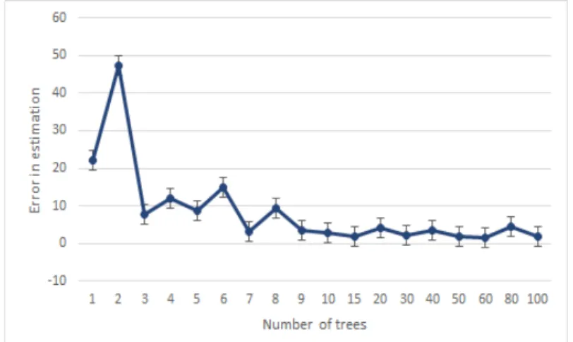
5.15 Number of successful health assessments with respect to the number of trees. . . 97
L
ISTE DES TABLES
2.1 DoS attacks for different network layers [Wood et al., 2002] . . . 23
3.1 Comparison of maintenance strategies. . . 34
3.2 Some definitions of prognostics reported in the literature. . . 37
3.3 Classifying models in the literature. . . 40
3.4 An overview of Prognostic models. . . 49
5.1 Simulation characteristics. . . 88
I
S
TATE OF THE ART AND
I
SSUES
1
G
ENERAL INTRODUCTION
D
uring their life cycle, and from the moment of their deployment, industrial systemsare subjected to failures. A failure might be irreversible or have undesirable outcomes with consequences varying from minor to severe. Generally speaking, system failure can lead to :– An interruption of service. The service can be critical and even a brief stoppage could degrade the quality of response or prevent the system from providing the intended output.
– Money loss, like the case of grounded airplanes where the loss counts in millions of dollars. Extra costs can also be related to system repair.
– Jeopardizing the security of the users in case of severe outcomes (fires, explosions, gas leaks, etc.), not to mention endangering the environment.
An illustration of the severe consequences is given in Figure11.1.
In the 21st century alone, many notable industrial disasters took place. For instance, in
the defense industry, an incident occurred on July 11th2011 in Zygi, Cyprus (see Figure
1.1(c)). 98 containers of explosives self-detonated after being stored for two and a half years in the sun. The explosion killed 13 people and injured 62 others. Hundreds of nearby buildings and the island’s largest power station were damaged. The costs of this explosion were valued at 10% of the country’s economy, which is equal to 3.822 American billion dollars.
On July 6th2013, a derailment of a runway train took place in Quebec (see Figure 1.1(a)).
A combination of neglected defective locomotive, poor maintenance, driver error, flawed operating procedures, weak regulatory oversight, and lack of safety redundancy caused the death of 42 victims and 5 other people were presumed dead. More than 30 buildings were destroyed, while 36 were demolished due to contamination. 115 businesses were either destroyed, displaced, or rendered inaccessible. Claims to local insurers were esti-mated at a total of $ 50 million.
The Deepwater Horizon oil spill (see Figure 1.1(b)), which happened in Gulf of Mexico from April 20th until July 15th 2010, killed 11 individuals and 143 spill-exposure cases
were reported to the local hospital. This was caused by a wellhead blowout, and the well was officially sealed only on September 19th2010. The spill volume was estimated at 4.9
million barrels spreading on an area of 6,500 to 176,100 Km2. This cost the company
about $ 65.425 billion between fines and settlements.
1. Images courtesy (a,d) wikipedia.org, (b) nypost.com, (c) CyprusNewsReport.com
TransAsia Airways Flight 235 (Figure 1.1(d)) is a domestic flight that crashed on February 4th 2015 shortly after takeoff from Taipei Songshan Airport. The aircraft’s right engine triggered an alarm just 37 seconds after takeoff. Whereas the crew reported a flame-out, data showed one of the engines had in fact been moved into idle mode. Soon the right engine failed to produce enough thrust for its rotating propeller, lapsing into auto-feathering. A restart was attempted, but the aircraft crashed 72 seconds later. From 58 passengers and crew members on board, 43 were killed. The remaining 15, in addition to 2 victims on ground, were injured. Right after the crash, 100 flights were canceled. So far, this has caused the company around US$ 475,000 as fees of compensation to the families of the deceased.
(a) Lac-Mégantic rail disaster, Quebec. (b) Deepwater Horizon oil spill, Gulf of Mexico
(c) Evangelos Florakis Naval Base explo-sion, Cyprus.
(d) TransAsia Airways Flight 235, Taiwan.
FIGURE1.1 – Examples of failure outcomes.
The human casualties cost the plants the trust of their clients, which reduces dramati-cally their equities and incomes. Production stoppage and repair durations also generate countless money loss and expensive fees. From this context, it is important to monitor the system, assess its health, and plan maintenance activities preferably before the system fails.
Maintenance is an important activity in industry. It is performed either to revive a ma-chine/component, or to prevent it from breaking down, and aims for increasing system availability, readiness and enhancing safety. Different strategies have evolved through time, bringing maintenance to its current state. This evolution was due to the increasing demand of reliability in industry. Nowadays, plants are required to avoid shutdowns while offering safety, availability, and reliability, all while reducing the costs.
5
The first form of maintenance is the corrective one. In this strategy, actions are only taken when the system breaks and no longer can perform the intended tasks. These actions could be equipment repair or replacement. The corrective maintenance reduces the cost of manpower related to maintenance actions. However, plants cannot afford to undergo breakdowns. In fact, sudden shutdowns cost money due to the interruption of produc-tion and time due to repair activities. A component failure, in some cases, can lead to a secondary failure, worsening the situation and elevating the costs.
As a remedy to these issues, maintenance became a periodic activity. Domain experts rely on their knowledge and the observation of upcoming events to set time intervals in which the components are inspected and replaced if needed. This preventive main-tenance is especially adopted by transportation and nuclear plants [Hu et al., 2012]. A time-based maintenance will encompass any action that aims at adjusting signs of de-terioration, in a way that stretches the time interval until a failure occurs. This strategy reduces the occurrence of system breakdowns and increases reliability. The main draw-back of preventive maintenance is the fact that it is performed regardless of the machine’s condition. In other words, industrials have to hire domain experts in order to set intervals for maintenance. Sometimes, these intervals are irrelevant as the machine can be in a healthy state and this will cost extra and avoidable fees. Besides, even with periodic maintenance and inspections, random failures still occur. This is why Condition Based Maintenance (CBM) was proposed and developed in early nineties [Heng et al., 2009]. CBM is based on real-time observations. It is an online approach that assesses machi-ne’s health through condition measurements. As any maintenance strategy, CBM aims at increasing the system reliability and availability while reducing maintenance costs. The benefits of this particular strategy include avoiding unnecessary maintenance tasks and costs, as well as not interrupting normal machine operations [Heng et al., 2009]. CBM de-creases the number of maintenance operations and causes a reduction of human error influences.
A new maintenance has recently emerged : Predictive Maintenance (PM). It predicts the system health in the future, based on the current condition, and defines the needed main-tenance activities accordingly. This way, the system is only taken out of service if a direct evidence exists that deterioration has actually taken place. This increases maintenance efficiency and productivity on one hand, and decreases maintenance support costs and logistics footprints on the other.
Figure 1.2 summarizes this evolution of maintenance strategies through time.
In order to shift from traditional maintenance strategies to CBM and PM, extra tasks are required. These tasks encompass system surveillance, data analysis and modeling, and decision making support system. This scientific approach is called Prognostics and Health Management (PHM).
Over the past years, research in PHM field has gained a great deal of attention. Pro-gnostic models are developed in an attempt to predict the Remaining Useful Life (RUL) of machinery before failure takes place. This is done following the steps described in Figure 1.3.
A reliable prediction activity requires continuous online measurements of the operating conditions of the system under consideration. This information is usually gathered by means of sensor nodes. Sensory data are reported periodically to monitor the critical components. The data packets contain signals that correspond to measurements of
mo-FIGURE1.2 – History of maintenance strategies.
FIGURE1.3 – PHM general steps.
nitoring parameters such as pressure, temperature, moisture. . .
This information is used for a comprehensive analysis of the system behavior. This com-prehension will help build models to assess the health, diagnose the system, and ex-trapolate the results in the future to estimate the time before failure. After these steps being achieved, the decision making support system will help the user plan the neces-sary maintenance actions if needed. However, if the prediction model and the provided measurements are not accurate, it is possible that the maintenance activity will be perfor-med either "too soon" or "too late". This is illustrated in Figure 1.4.
1.1. POSITIONING OF THE RESEARCH 7
FIGURE1.4 – Maintenance activity.
1.1/
P
OSITIONING OF THE RESEARCHPHM can be performed through one of four main approaches : (i) model-based ap-proach, (ii) knowledge-based models, (iii) data-driven models, or (iv) hybrid models. Model-based approaches rely on a mathematical representation of the component re-sponding to stress. Although the model is reliable, it requires intensive experimentation and verifications and could only be built by a domain expert. Knowledge-based models also explore domain experts’ experience to derive models from rules built upon obser-vations. This approach’s complexity grows exponentially with the number of the derived rules. Data-driven approaches are used when the first principles of the system opera-tion are too complex to develop an accurate model of physics of failure. Finally, hybrid approaches combine two different approaches among data-driven, model-based, and knowledge-based approaches. This combination will leverage the advantages of each one of the used approaches. However, these models could be computationally expensive as well as complicated to develop.
In data-driven approaches, models are directly derived from condition monitoring data, based on statistical and stochastic learning techniques. These models have a double role : assess current operating conditions and predict the RUL. Neither human expertise nor comprehensive system physics are needed for the model building process.
A data-driven approach transforms raw data provided by the monitoring system into useful information. By means of this information and historical records, a behavioral model is built and predictions can be performed. In this thesis, we develop a data-driven approach for on-line health assessment using the Random Forest algorithm (RF).
To the best of our knowledge, existent research works in PHM perform data collection either by means of individual sensors, or via wired networks of sensor nodes. In some monitoring applications, the deployment of a Wireless Sensor Network (WSN) is manda-tory rather than a choice for the following reasons.
– Due to accessibility restrictions, it is sometimes easier to place wireless sensors in the monitoring area, without the constraint of connecting them with wires.
– Some systems are sensitive to extra weight, and eliminating the wires can guarantee better performances.
– We can get closer to the source of the data we need, comparing to when we use wires, it can also become easier to deploy more sensors in the monitoring process, and thus get more precise values.
For precision and feasibility purposes, we consider in this study the case where the nodes communicate their information within a WSN.
Two of the most hot topics related to WSN are energy consumption and network reliability. Energy consumption can be optimized through the choice of topology, the deployment of the routing protocol, and node scheduling. In this thesis we investigate different topolo-gies to illustrate their impact on the quality of data. We also propose a node scheduling scheme that keeps a minimum number of sensor nodes in the active mode while ensuring coverage.
Network reliability solutions aim at improving the network availability (by employing fault tolerance techniques) and minimizing packet loss. However, this does not completely eliminate the risks of loosing information. Our proposed algorithm stores copies of the sensed data into the neighboring nodes memory. These copies are retrieved once the sender fails before delivering the data packet. The data packets arrived at the sink node will later be used for PHM.
A majority of the current research works in PHM study the accuracy of models from the angle of improving prognostics algorithms only. In this thesis, we focus our attention on earlier steps, namely : (i) data acquisition, (ii) data processing, (iii) and health assess-ment.
The quality of the available data for the PHM process is not always considered in the literature. The solutions proposed in the literature are based upon the assumption of completeness and correctness of data. This assumption, however, is far from being true especially in the case of WSN monitoring. Therefore, we focus our attention on a data-driven approach that can adapt to the change of quality of the monitoring data. More precisely, we use the random forest algorithm for health assessment.
1.2/
R
ESEARCH QUESTIONSWSN monitoring is somehow unique in the sense that the sensors are also subjected to failures or energy exhaustion, leading to a change in the network topology. Thus, mo-nitoring quality is variable too and it depends on both time and the location of sensors on/around the device. Our challenges conducting health assessment, while monitoring the system with a WSN, arise as follows :
– Data acquisition step : how is the data being gathered ? Which routing protocol is em-ployed ? Which topology is best ?
– Data processing step : is the data complete ? Is the amount of data at the base station sufficient for health assessment ?
– Health assessment step : In the light of the monitoring constraints, how can we estimate the health state ?
Various strategies can be deployed on the network to achieve fault tolerance or to extend the WSN’s lifetime, like nodes scheduling or data aggregation. However, the health as-sessment process must be compatible with these strategies, and with a device coverage of a changing quality. Another challenge related to this work, is finding an algorithm that adapts to the change in number of sensors.
1.3. GLOBAL ASSUMPTIONS 9
1.3/
G
LOBAL ASSUMPTIONSData-driven approaches consist in a machine learning algorithm to understand the de-gradation mechanism of the system in question. The input of such an algorithm would be sensor measurements describing the degradation of the system over time. A challenging step in a data-driven approach is data gathering. Actually, the quality of sensor data af-fects the efficiency of the health assessment process. A prior study by system experts is needed to ensure a strong basis for reliable models. The global assumptions considered in this research work are as follows.
1. The optimal number of sensor nodes, their location, and the parameters to be mo-nitored are previously determined by system experts.
2. Data acquisition begins when the system starts functioning and stops only when it completely fails or all sensors have exhausted their energy resources.
3. During data acquisition, no maintenance activity takes place. 4. The degradation develops gradually over time.
5. Data is ready for use.
6. The network used for the monitoring activity is secured.
1.4/
C
ONTRIBUTIONS OF THE THESISWSNs are designed for the purpose of an efficient event detection. They consist of a large number of sensor nodes deployed in a surveillance area to detect the occurrence of possible events. Such an activity necessitates efficiency, which is hard to achieve with the constraints of WSNs. A prerequisite in PHM is to consider that data provided by sensors are either flawless or simply noisy, which is far from the truth. We, therefore, studied some aspects of WSN dependability. We studied different settings of the WSN. We showed that altering the topology has an impact on the quality of data arriving at the base station for health assessment. We also developed a fault tolerant technique, enabling the network to fulfill its intended task even in the presence of faults. Thus, there will be no interrup-tions in forwarding data for health assessment purposes. A data recovery process is also developed, it aims at reducing data loss by creating copies of packets in non-exhaustive way. A node scheduling scheme is included in the algorithm and it helps to improve the energy consumption.
In this thesis, the use of random forests (RF) is proposed for industrial functioning health assessment, particularly in the context of devices being monitored using a wireless sen-sor network (WSN). In the offline phase, the algorithm selects the relevant features for the best split in the decision tree, starting from the root until the leaf nodes are reached. This process is repeated until the maximum number of trees is reached. The algorithm, since it is based on random selections, has the advantage of starting from different points (or distributions). Therefore, in the online phase, this can be beneficial for mainly two reasons :
– Health assessment can be performed considering the relevance of all features. A ma-jority vote will then assign the correspondent health class, and this reduces errors.
– If one feature is missing (due to sensor error), the health assessment process will not be interrupted as other trees have a different starting point.
To summarize, the contribution of this research work is performing health assessment with WSN monitoring, render the network more reliable, and improve the quality of predictions by focusing on the early steps of the process. The proposed solution is summarized in Figure 1.4.
FIGURE1.5 – The overall scheme of the proposed solution.
1.5/
P
UBLICATIONS1.5.1/ PUBLISHED PAPERS
1. Dependable wireless sensor networks for prognostics and health management : a survey. Annual Conference of the Prognostics and Health Management Society, PHM’14, / Fort Worth - Texas - USA (Volume 68, 2014, Pages 1-15). Wiem Elgha-zel, Kamal Medjaher, Christophe Guyeux, Mourad Hakem, Noureddine Zerhouni, Jacques Bahi.
2. Random Forests for Industrial Device Functioning Diagnostics Using Wireless Sen-sor Networks. IEEE AEROSPACE CONFERENCE, 2015. / Big Sky, Montana, USA (2015, Pages 1-9). Wiem Elghazel, Jacques Bahi, Ahmad Farhat, Christophe Guyeux, Mourad Hakem, Kamal Medjaher, Noureddine Zerhouni.
3. Dependability of wireless sensor networks for industrial prognostics and health ma-nagement. Computers in industry (Volume 68, January 2015, Pages :1-15). Wiem Elghazel, Jacques Bahi, Ahmad Farhat, Christophe Guyeux, Mourad Hakem, Kamal Medjaher, Noureddine Zerhouni.
1.6. THESIS OUTLINE 11
1.5.2/ SUBMITTED PAPERS
1. Resiliency in Distributed Sensor Networks for Prognostic and Health Management of the Monitoring Targets. Jacques Bahi, Wiem Elghazel, Christophe Guyeux, Mo-hammad Haddad, Mourad Hakem, Kamal Medjaher, and Noureddine Zerhouni. Submitted to the computer journal, Oxford.
2. Reliable diagnostics using wireless sensor networks. Wiem Elghazel, Jacques Bahi, Christophe Guyeux, Mourad Hakem, Kamal Medjaher, Noureddine Zerhouni. Submitted to Journal Européen des Systèmes Automatisés.
3. Health assessment with incomplete data using wireless sensor networks. Wiem El-ghazel, Jacques Bahi, Christophe Guyeux, Mourad Hakem, Kamal Medjaher, Nou-reddine Zerhouni.
Submitted to IEEE Sensors Journal.
4. Data recovery and energy efficiency in distributed wireless sensor networks. Jacques Bahi, Wiem Elghazel, Christophe Guyeux, Mohammad Haddad, Mourad Hakem, Kamal Medjaher, and Noureddine Zerhouni.
Submitted to INFOCOM 2016.
1.6/
T
HESIS OUTLINEThe remainder of this thesis is organized as follows :
Chapter 2 presents an overview of wireless sensor networks and their advantages. It also states the weaknesses of this type of networks, to better understand what threatens the quality of service. Some of the solutions to reach network’s dependability reported in the literature are listed.
Chapter 3 compares the different maintenance strategies that evolved through time. Condition-based maintenance is put under the spot light and useful definitions regar-ding prognostics and health management are given. Various prognostics approaches are explained and discussed while highlighting each of their advantages and drawbacks, in a way that justifies the choice of data-driven approaches. This chapter also discusses the challenges of wireless sensor networks monitoring in the context of industrial prognostics and health management. Finally, this chapter emphasizes what needs to be tackled for the purpose of obtaining good results.
Chapter 4 presents a distributed algorithm for resiliency in wireless sensor networks. The algorithm has two main goals : (1) reducing energy consumption in the network and (2) recovering data loss. The algorithm consists in a node scheduling mechanism. This mechanism not only ensures that only one sensor node is active per area, but also that each area is covered at all times (as long as there still exist alive nodes). An area is delimited by a distance equal to the nodes’ radio range. Two different mechanisms for data recovery are proposed, depending on whether memory constraints exist or not. Chapter 5 proposes the use of the random forest algorithm for health assessment. The algorithm is used to identify the health state of an industrial device when the monitoring parameters are incomplete. This method is validated through computer simulations while varying the data collection process.
Chapter 6 summarizes the work that was achieved and enumerates the contributions of this thesis. It also discusses the limitations and the perspectives.
2
A
N OVERVIEW OF WIRELESS SENSOR
NETWORKS
W
ireless Sensor Networks (WSN) are a new technology that appeared in the nineties.The emergence of WSN is the result of the advancement in low cost wireless com-munication and micro electro mechanical systems [Akyildiz et al., 2002]. These networks became wild spread thanks to their easy deployment and their low cost. In the past, get-ting data transferred from one unit to another requested expensive wiring. Nowadays, we can place nodes almost anywhere, having no wiring contrasts, with any geographic or emplacement problems, and this is due to the minimal batteries feeding the nodes. The sensors’ small dimensions give them the advantage to be used even discreetly. These ad-vantages allowed WSN to be deployed in various fields, such as : agriculture, medicine, home automation, military, etc.Typically, a WSN is composed of few base stations (one in most cases) and hundreds (or thousands) of sensor nodes. The main role of these devices is to monitor physical or environmental conditions, and cooperate to deliver the sensed data to a base station called the sink.
WSN are composed of very small sensors with very limited and nonrenewable energy. In order to preserve this energy, network throughput has to be low. Furthermore, as all wireless networks, WSN are not very secure. A node can easily be hacked or failed, either due to energy limitation or to network mobility. Moreover, they do not dispose with a predefined infrastructure and this fact highlights the importance of the chosen routing protocol. An adequate protocol should ensure a reliable communication. This reliability means reducing data loss, fastening communication, minimizing energy consumption, and other standards.
WSN are event-based systems that rely on the collective effort of several sensor nodes [Akan et al., 2005]. This offers the network greater accuracy, larger coverage area, and the possibility to extract localized features. The network extends the computational capa-bility to physical environments that human beings cannot reach. Generally, sensor nodes are not located far from each other (since they function at a low frequency). As a conse-quence, it is highly possible that many nodes sense the same data. And if all this redun-dant information is routed through the network, useful energy will be dissipated in vain. In this chapter, a general overview of WSN is provided. This encompasses their advan-tages, drawbacks, and the solutions implemented to improve their performance.
2.1/
D
EFINITIONSA sensor node is a tiny device having the capability of sensing new events, computing the sensed and received values, and communicating information. Thus, the network can be deployed to monitor physical and environmental phenomena such as temperature, vibrations, light, humidity, etc.
As shown in Figure 2.1, the node is equipped with a sensor, a data processing unit, a memory space, a radio range, and a battery.
FIGURE2.1 – Components of a sensor node
Ad hoc is the Latin for "for this", and it means a non-generalizable solution designed for a specific problem or task.
A WSN is an ad hoc network as it does not rely on a pre-determined infrastructure. Each node participates in routing the packets by forwarding data for other nodes determined dynamically on the basis of network connectivity.
WSNs can be either heterogeneous or homogeneous [Li et al., 2011]. In the latter, all nodes have the same role and characteristics. In the former, nodes have different roles : some nodes simply sense and forward information while others aggregate data, manage their area, perform computations. . . Consequently, some of the nodes can be equipped with higher energy, longer radio range. . .
There are different settings for a WSN, which is generally dynamic as radio range and network connectivity change over time [Li et al., 2011]. The most used WSN models are hierarchical, distributed, centralized, or decentralized (Figure 2.2).
In the distributed topologies, there is no central node managing the network (or a region of it). They consist in a collection of nodes having equal roles. Therefore, no aspect of hierarchy is considered. Before the network starts running, no prior infrastructure is im-posed ; each node discovers its surrounding area and decides which node (or nodes) to communicate with. This decision usually relies on the radio range and the transfer dis-tance. With this topology, it is easy to add new sensor nodes to the network ; as they only need to establish links with their neighbors. Distributed topologies render the network’s maintenance an easy task : should a node fail, its neighbors will establish new links with other nodes within their sensing range, and the network will continue to work normally. Nevertheless, this topology may result in extra costs related to energy consumption and security codes.
2.1. DEFINITIONS 15
(a) Distributed topology (b) Hierarchical topology
(c) Centralized topology (d) Decentralized topology
FIGURE2.2 – Network topologies
Sensor nodes can be organized in several levels, making a hierarchical topology (or a tree topology). The root represents level 0 and there is no level above. Sensor nodes from two adjacent levels are connected in an end to end manner. The hierarchical model can be seen as three different layers : (1) the core layer (the root), which is optimized for availa-bility and performance, (2) the distribution layer, which implements policies and forwards messages, and (3) the access layer (the leaf nodes), which represents the access point to the network. Hierarchical WSN have the advantage of being scalable. The presence of different levels makes the network more manageable and simplifies the task of isolating and detecting faults. Unfortunately, when the network spans on a great area, maintenance can be an issue. If a parent node fails, its children can no longer communicate with other nodes in the network. Apart from leaf nodes, any node failure in the network will result in disjoint sub-trees.
One of the easiest topologies to design and implement is the centralized topology (also called star topology). All the sensor nodes have the simple task of sensing new informa-tion and forwarding it to a central node where all the data processing will be proceeded with. Adding new nodes to the topology is a simple task ; the central node is known and only a connection with the new sensor needs to be established. One of the major pro-blems of this topology is that it presents a single point of failure. If a problem occurs at the central node, the whole network becomes paralyzed : when a new event is detected, the
data packet cannot be forwarded nor processed. The network loses purpose once it loses its central node. In addition to this, the network does not ensure speed. In fact, increasing the network’s density will lead to higher traffic. An important number of forwarded packets towards the same point may result in a traffic jam and packets collision, known in this case as the bottleneck problem.
Decentralized topologies can be seen as a combination of the distributed and the cen-tralized topologies. The network is divided into regions (or clusters) which are locally managed by a central node (called the Cluster Head CH). This topology is best known for offering a reasonable compromise between energy consumption and Quality of Service (QoS). Adding new nodes and managing the topology would be as simplified as in the centralized topologies. In the same time, the congestion problem is reduced and the net-work no longer has a single point of failure. However, once a CH fails, the corresponding area is no longer monitored.
Choosing a network setting depends on the target application (mainly its goals and li-mits), and the routing protocol will be developed accordingly. The protocol stack of sensor networks is composed of five different layers [Akyildiz et al., 2002], which are shown in Figure 2.3.
FIGURE2.3 – Protocol stack for WSN.
1. Physical layer : it defines the means of transmitting data packets after being conver-ted into raw data bits, that are suitable for transmission over the communication medium. Mainly, this layer is responsible for frequency selection, carrier frequency generation, signal detection, modulation, and data encryption.
2. Data link layer : It is charged of data stream multiplexing, data frame creation, me-dium access, and error control to provide reliable transmission. it is also charged of the creation of the network infrastructure, transferring data, and fairly and efficiently sharing the communication resources between sensor nodes, in order to achieve good network performance in terms of energy consumption, network throughput, and delivery latency. It is also responsible for error control of transmission data. 3. Network layer : it is responsible for routing the data from the source nodes until the
2.2. WIRELESS SENSOR NETWORKS FOR INDUSTRIAL MONITORING 17
can be used as a gateway. It commands and controls the system, forwards data packets, and takes charge of routing between intermediate routers.
4. Transport layer : it is responsible for end-to-end data delivery between sensor nodes and the sink. Due to energy, computation, and storage constraints, traditio-nal transport protocols cannot be applied directly to WSNs. This layer also provides other services such as multiplexing, reliability, flow control, congestion avoidance... 5. Application layer : it includes a variety of protocols that perform various sensor ap-plications, such as query dissemination, node localization, time synchronization, network security, etc. It can be defined as the user interface. It displays messages in a human recognizable and understandable format.
Due to their low cost, their easy deployment, and their capacity to extract localized fea-tures, WSN are widely spread. Nowadays, we can find them nearly in all monitoring appli-cations. However, to the best of our knowledge, the use of this technology is not reported in the literature of Prognostics and Health Management (PHM). Nevertheless, in some industrial applications, the WSN monitoring can be mandatory. This is further explained in the next section.
2.2/
W
IRELESSS
ENSORN
ETWORKS FORI
NDUSTRIALM
ONITO -RINGThe monitoring activity begins with the simple question : how many sensor nodes do we need ?
First of all, the number of sensors depends on the number of monitored parameters. The sensors have different types, so for each of the monitored parameter, we need at least one sensor for the monitoring activity. Secondly, for large systems, more than one strategic place can be found to extract localized values for the parameter under consideration. Therefore, situations where more than one sensor node is needed are very common. Once we have determined the number of sensors, the second question we ask ourselves is : how is the collected data routed to the base station ?
Most of the encountered research works use individual sensors for data collection. This means that each sensor transfers its sensed data to the base station (BS) separately. Once at the BS, the data packets are processed and fusion algorithms are deployed to extract correlations.
As long as the number of sensors is limited, wiring should not be a problem. But as their number grows higher, connecting the sensors individually to the BS starts to turn into a complicated task. An alternative solution would be connecting the sensors in a hop by hop manner until reaching the final destination (which is th BS). A hop is a portion of the path between the source (sender) and the destination. In a hop by hop communication, the packets are sent from one node to the other until reaching the BS. Therefore, only the nodes that are the closest to the BS are directly wired to it. This should reduce the costs and renders wiring less complicated.
However, even with this solution, wiring can still remain a complicated task. Here for example, we take the case of wind turbines shown in Figure1 2.4. A wind farm usually
contains a number of wind turbines that can be over one hundred in some cases. Connec-ting the sensors monitoring each of the wind turbines via wires is not that easy, especially when we face the facts. Wind turbines should be spaced by about 6 to 10 times the dia-meter of the rotor. Modern wind turbines have diadia-meters varying from 40 to 90 dia-meters. So, in best case scenario, connecting two sensors in adjacent wind turbines would require a wire of 240 meters long, at least ! Connecting each of the wind turbines directly to the base station is clearly worse, and performing localized processing will add the constraint of access, like the case of offshore wind farm in Figure 2.4(c).
Putting this aside, let us have a look at the wind turbine design in Figure 2.4(b). We can see that the generator component is composed of several parts in constant rotation. Adding wires to the equation would clearly complicate things even more.
(a) A field of wind turbines. (b) Components of a horizontal-axis wind turbine.
(c) Wind turbines set offshore.
FIGURE2.4 – An example of wind turbines.
The drawbacks of wired networks can also be illustrated by the example of aircraft moni-toring. In Figure 2.5 are shown two examples of sensor networks on a Boeing 7772, and on an Airbus3.
In a study conducted by the Sahara project4, it is stated that an Airbus A380 has 500 miles of cable with a total weight that exceeds 3 tons. The use of WSNs would save at least hundreds of pounds, and thus reduces the consumption of fuel.
Implementing a WSN has a number of advantages that we can summarize as : (i) giving an easier access to extract localized features, (ii) granting access in case of geographical difficulties, (iii) reducing the complexity of manufacturing and associated hazards, and (iv)
2. Image courtesy : Institute of fluid-flow machinery, Polish academy of science
3. Image courtesy : High performance composites- Article : Structural health monitoring : Composites get smart
2.3. SHORTCOMINGS OF A WSN 19
(a) WSN on a Boeing 777. (b) WSN on an Airbus.
FIGURE2.5 – airplanes.
eliminating faults related to wired communication (such as delays). Unfortunately, a WSN also has limitations which are reviewed hereafter.
2.3/
S
HORTCOMINGS OF AWSN
WSNs are designed for the purpose of an efficient event detection. They consist of a large number of sensor nodes deployed in a surveillance area to detect the occurrence of new events. Such an activity necessitates efficiency, which is hard to achieve with the constraints of WSNs. These limitations are detailed in the following.
2.3.1/ RESOURCES
Available energy is a big limitation to WSN capabilities. The sensors are small sized devices, which results tiny batteries as energy supply. Moreover, the nodes are often deployed in hostile environments (mountains, enemy territory...). So once deployed, they cannot be recharged [Carman et al., 2000].
The added security code has an important impact on the available energy for normal network tasks. Processing security functions (encryption, decryption, signing data, veri-fications), transmitting security related data (vectors for encryption/decryption), and se-curing storage (cryptographic key) necessitate extra power, which is critical for WSNs [Carman et al., 2000, Walters et al., 2007].
In addition to this, the deployed memory space for a sensor node is very limited. The storage space is shared between the communication protocol and the security code. The size of the latter has then to be limited to a minimum [Walters et al., 2007].
Buffering space in sensor nodes is also limited. This will lead to packet loss with the increase in traffic flow towards the sink node. In fact, a data packet cannot be held by the sensor for a long period with new packets coming in. In the case of a high traffic flow, all the nodes will attempt to « get rid » of the old messages in order to make space to the new ones, by forwarding them to the next level. Therefore, the area around the sink tends to be quickly congested as all sensor nodes tend to forward the captured data to the sink.
2.3.2/ COMMUNICATION
Wireless communication is known to be unreliable and it adds to the network’s vulnerabi-lities. The absence of physical connections can result in :
– Channel errors : Due to noise in the communication channels, the arrival of wrong signals may occur at the recipient.
– Missing links : Route updates, interference in the radio channels, energy exhaustion... lead up to invalid or missing links between the sensors and consequently to packet drop.
– Network congestion : Heavy traffic is reflected by a dense packet exchange in the network, and a concurrent access may present itself at certain regions. When a node carries so much data, its QoS degrades as this leads to packet collision, packet loss, transmission delays...
– Communication latency : Multi-hop routing and node processing both lead to a great latency. Latency is the time elapsed between packet sending and packet reception. When transmission errors require retransmissions, extra delays are to take into consi-deration. One of the major drawbacks of latency is that it makes synchronization among nodes hard to achieve.
Most WSNs are deployed in harsh environment conditions and/or are exposed to adver-sary attacks. This emphasizes the likelihood of physical attacks, which can cause perma-nent (even irreversible) damage to the hardware. Since the network is managed remotely, the sensor nodes can be left unattended for a long period of time. It is therefore difficult to detect physical tampering or perform regular maintenance, and thus, the network would remain unable to fulfill the intended tasks [Walters et al., 2007].
Routing solutions in WSNs avoid central management point as it results in a single point of failure. This complicates the synchronization among nodes, and lowers packet delivery rate. Ensuring synchronization among nodes necessitates access to extra memory space to improve the communication protocol, consuming more resources.
2.3.3/ COVERAGE AND LIFETIME OPTIMIZATION
Considering all the limitations mentioned above, it is not easy for the network to always fulfill the intended tasks. Reliability and efficiency of WSNs are dependent on key issues, which are enumerated in the following.
2.3.3.1/ COVERAGE
Sensor nodes have a short radio range and they collaborate to cover a given surveillance area. At the network setup phase, it is crucial to ensure that the network is configured in a way that it covers all the area [Tian et al., 2005]. The coverage problem arises as : how to ensure that, at any time, any zone in the network is covered by at least one sensor node ?
[Zorbas et al., 2007] presented B{GOP}, a centralized coverage algorithm for WSNs. The algorithm proposes sensor candidate and avoids double-coverage depending on the co-verage status of the corresponding field.
2.3. SHORTCOMINGS OF A WSN 21
[Wang et al., 2003] presented a protocol that can dynamically configure a network to achieve guaranteed degrees of coverage and connectivity. They gave a proof that sensing coverage range does not need to be more than half the connectivity range in the network. Thus, their protocol helps preserve energy while maintaining coverage in the network. In [Hefeeda et al., 2010], a general coverage algorithm, which considers the network connectivity, is presented. The proposed protocol, called Probabilistic Coverage Proto-col (PCP), works for the common disk sensing model as well as probabilistic sensing model. To support probabilistic sensing models, the authors introduce the notion of pro-babilistic coverage of a target area with a given thresholdθ, which means that an area is considered covered if the probability of sensing an event occurring at any point in the area is at leastθ. They prove the correctness of the protocol and provide bounds on its convergence time and message complexity.
2.3.3.2/ AWAKE NODESvs SLEEPING NODES
In order to prolong the network’s lifetime, a possible solution is to keep a minimum number of sensor nodes in active mode. As WSNs rely on nodes density in the sensing and communicating processes, it is very likely that some nodes will not be needed. If a reliable node can forward data packets toward the sink, its neighbors can switch to idle state temporarily.
Lifetime optimization using knowledge about the dynamics of stochastic events has been studied in [He et al., 2012b]. The authors presented the interactions between periodic scheduling and coordinated sleep for both synchronous and asynchronous dense sta-tic sensor network. They show that the event dynamics can be exploited for significant energy savings, by putting the sensors on a periodic on/off schedule.
In [He et al., 2012d], the authors design a polynomial-time distributed algorithm for maxi-mizing the lifetime of the network. They proved that the lifetime attained by their algorithm approximates the maximum possible lifetime within a logarithmic approximation factor. The authors in [Kasbekar et al., 2011a] leverage prediction to prolong the network life time, by exploiting temporal-spatial correlations among the data sensed by different sen-sor nodes. Based on Gaussian Process, the authors formulate the issue as a minimum weight sub-modular set cover problem and propose a centralized and a distributed trun-cated greedy algorithms (TGA and DTGA). They prove that these algorithms obtain the same set cover.
As sensor nodes periodically go to sleep, they need to be awake when they are re-quested to. This is done by the transmission of wake-up messages towards a target sensor. However, if the message is not received at the right moment, data packets will be dropped. This will cost the network extra energy due to packet retransmission [Ye et al., 2003, Gallais et al., 2006, Bahi et al., 2011].
2.3.3.3/ WEAR-OUT EFFECT
In WSN, if the wear-out failures are not taken into consideration during the execution of the involved application, some nodes may age much faster than the others and become the reliability bottleneck for the network, thus significantly reducing the system’s service
li-fetime. In the literature, this problem has been formulated and studied in various ways. For instance, prior work [He et al., 2012b, He et al., 2012d, Kasbekar et al., 2011a] in lifetime reliability assumes node’s failure rates to be independent of their usage times. While this assumption can be accepted for memoryless soft failures, it is obviously inaccurate for the wear-out-related fail-silent (a faulty node does not produce any output) and fail-stop (no node recovery) failures, because the sensor node’s lifetime reliability will gradually decrease over time.
To cope with this problem, a distributed self-stabilizing and wear-out-aware algorithm is presented in [Bahi et al., 2013]. This algorithm seeks to build resiliency by maintaining a necessary set of working nodes and replacing failed ones when needed. The proposed protocol is able to increase the lifetime of wireless sensor networks, especially when the reliabilities of sensor nodes are expected to decrease due to use and wear-out effects.
2.4/
A
TTACKS INWSN
SAs discussed before, WSNs suffer from limited computation capabilities, a small memory capacity, poor energy resources, absence of infrastructure, and susceptibility to physical capture. A variety of security solutions exists for infra-structureless networks (Ad hoc net-works). Yet, they do not all answer the security challenges of WSNs.
WSNs are vulnerable to many attacks, due to their uncontrolled environment of deploy-ment, the limitation of their resources, and the broadcast nature of the transmission me-dium. The attacks are mainly classified under two categories : physical attacks and non-physical attacks. In the following, we discuss some of the famous possible attacks in WSNs.
2.4.1/ NON-PHYSICAL ATTACKS
These attacks aim at disturbing the service and the normal operations in the network. In the following, examples of well-known non-physical attacks in WSNs are given.
2.4.1.1/ DENIAL OF SERVICE ATTACK
A Denial of Service (DoS) attack is an attempt to render the network unavailable to its users by leading to a server overload. It forces the network to either reboot or exhaust its resources, making it fail to perform the intended tasks. This attack is dangerous as WSNs lack the capacity to handle computational overhead to implement typical defensive stra-tegies.
The DoS attack can target the physical layer (jamming, tampering), the link layer (col-lisions, exhaustion, unfairness), the network and routing layers (neglection, greed, ho-ming, misdirection, black holes), or the transport layer (flooding, desynchronization) [Walters et al., 2007].
DoS attacks are very common. Therefore, there exist effective defensive measures against these attacks. Table 2.1 summarizes the possible defenses against different DoS attacks.
2.4. ATTACKS IN WSNS 23
Network Layer Possible Attacks Defenses
Physical Layer - Jamming - Spread-spectrum - Priority messages - Lower duty cycle - Region mapping - Mode change - Tampering - Tamper-proof
- Hiding
Link Layer - Collision - Error correcting codes - Exhaustion - Rate limitation
- Unfairness - Small frames Routing Layer - Neglect and Greed - Redundancy
- Probing - Homing - Encryption - Misdirection - Egress filtering
- Authorization - Monitoring - Black holes - Authorization
- Monitoring - Redundancy Transport Layer - Flooding - Client puzzles
- Desynchronization - Authentication
TABLE2.1 – DoS attacks for different network layers [Wood et al., 2002]
constraints of sensors. Their approach relied on two types of entropy estimators. A main estimator is charged of the synthesis of localized computations, whereas the other esti-mators are deployed hierarchically according to the network topology.
Wood and Stankovic [Wood et al., 2002] described an approach to defend against jam-ming. In a first step, the nodes surrounding the jammed area report their status to they neighbors. In a second step, the neighbors collaborate to identify the jammed region so they will not route packets through it.
2.4.1.2/ SYBIL ATTACK
The Sybil attack was defined by [Douceur, 2002] as « an attack able to defeat the redun-dancy mechanisms of distributed data storage systems in peer-to-peer networks ». A malicious device illegitimately takes on multiple identities to gain a large influence on the communication mechanism, by appearing and functioning as multiple distinct nodes. This attack is effective against routing algorithms, data aggregation, voting, fair resource allocation, and foiling misbehavior detection [Walters et al., 2007].
The Sybil attack is a harmful threat to sensor networks as it defeats redundancy mecha-nisms. To defend against such attacks, the network needs a mechanism to ensure that an identity is being held by one, and only one node in the network.
A light-weight identity certificate method is proposed by [Zhang et al., 2005]. This method avoids public key cryptography by using one-way key chains and Merkle Hash trees.
2.4.1.3/ TRAFFIC ANALYSIS ATTACK
Even with encrypted data, traffic analysis is able to determine what type of information is being communicated in the network (chat, requests...) and even falsify an identify and disable the base station [Walters et al., 2007]. A malicious node can generate a fake phy-sical event to be sensed. The attacker, then, will watch the activity of the nodes in the network ; nodes tending to forward more data packets are closer to the base station. Deng et al. investigate three techniques that aim at hiding the true location of the base sta-tion [Deng et al., 2004]. The first technique is multi-parent routing scheme. It introduces a degree of randomness in the multi-hop path from the source node until the base station. The second technique, called random walk, generates random fake routes to mislead an adversary while tracking the packet. And finally, fractal propagation consists in randomly creating multiple areas of high communication activities to disguise the true location of the base station.
2.4.1.4/ NODE REPLICATION ATTACK
In a node replication attack, an adversary can capture a sensor node, copy its ID, and insert a replica in the network [Parno et al., 2005].
The consequences of such an attack can be severe ; packets can be misrouted, changed, or corrupted, and significant parts of the network can be disconnected [Walters et al., 2007], etc.
[Parno et al., 2005] argue that previous node detection replication schemes depend either on centralized mechanisms or on neighboring voting protocols. Thus, they suffer either from single failure points or from failure to detect distributed replications. Considering these limitations, they propose two algorithms : randomized multicast and line-selected multicast. The line-selected multicast algorithm is inspired from the rumor routing descri-bed by Braginsky and Estrin in [Braginsky et al., 2002]. This algorithm helps reduce the communication cost of the randomized multicast protocol.
2.4.2/ PHYSICAL ATTACKS
In a WSN, adversary can perform the following physical attacks :
– Known-Plaintext Attack (KPA) : the attacker, having samples of both the plain text and the corresponding encryption, can reduce the security of the encryption key and reveal some of the information circulating in the network.
– Chosen-Plaintext Attack (CPA) : the attacker can choose a text to be encrypted. Doing so, it is easy to gain further information about the encryption key.
– Man-In-The-Middle Attack(MITMA) : the attacker creates a link between two nodes, through which they will communicate. The network cannot identify this connection as a malicious link. The attacker is then able to control the communication by intercepting and injecting messages.
2.5. DEPENDABILITY OF A WSN 25
2.5/
D
EPENDABILITY OFA WSN
The dependability of a WSN is a property that integrates the attributes needed for the application to be justifiably trusted. Such a network should be able to deliver a correct service, i.e., a service that implements the system’s function, and makes sure that a failed component will not lead to system failure. System dependability was defined by [Avizienis et al., 2000] as « the ability of a system to avoid failures that are more frequent or more severe, and outage durations that are longer, than is acceptable to the users ». In the following, we go through what the threatens the network’s dependability, how to evaluate it, and how we can attain it.
2.5.1/ THREATS
Developing a dependable WSN starts with defining the dependability requirements of users. In order to satisfy these needs, it is crucial to understand what might stop the network from delivering a correct service. In this section, the threats that can affect the dependability of a WSN are enumerated.
2.5.1.1/ FAULTS
A fault is the cause of an error, and it indicates a defect in the system. Its presence does not systematically lead to a failure. A fault is considered to be active only when it produces an error of one or more components. It is considered as transient if it affects the communication links between the nodes, and permanent if it is caused by hardware malfunction [Silva et al., 2012].
In [de Souza et al., 2007], the authors classify the sources of faults under two main cate-gories : node faults (related to hardware) and network faults (related to routing). A fault can have various origins, which are classified in Figure 2.6.
2.5.1.2/ ERRORS
An error takes place at run-time when some parts of the network enter in an unexpected (invalid) state that might result in a subsequent failure or undesirable outcomes. Such states are called hazards. As errors are hard to observe, special tools, such as debuggers, are required to declare their presence. An error indicates a discrepancy between actual behavior and intended behavior inside the network. It can then be detected if an error message or signal indicate its presence. If not detected, the error is called latent error [Avizienis et al., 2000, Taherkordi et al., 2006].
2.5.1.3/ FAILURES
A network failure is the observable consequence of an error. It occurs when the delivered service is no longer correct. The opposite transition (from incorrect to correct service) is called network restoration. Yet, the alteration of the service is not considered as a
FIGURE2.6 – Fault classes.
network failure until it reaches the service interface. With the implementation of fault to-lerance techniques, a network failure can be avoided even when an error is activated [Avizienis et al., 2000, Silva et al., 2012]. The possible failure modes are outlined in Fi-gure 2.7.
2.5.2/ ATTRIBUTES
This section deals with the ways by which we assess the dependability of a system. The attributes of dependability can vary in number and degree of importance considering the nature of the application and the intended service. The network, thus, is made depen-dable by adjusting the balance of the techniques to be employed according to the user’s needs.
2.5.2.1/ AVAILABILITY
In the classical definition, a network is considered as highly available if its downtime is very limited. This can be due either to few failures, or to quick restarts when fai-lures take place [Knight, 2004, Taherkordi et al., 2006]. If we add the security aspect, we can define availability as readiness for correct service for authorized users. This attri-bute can be computed as the probability that the network is functioning at a given time [Silva et al., 2012].
2.5.2.2/ RELIABILITY
A reliable network is a network that is able to continuously deliver a correct service. It can also be defined as the probability that a network functions properly and continuously in a time interval [Silva et al., 2012, Taherkordi et al., 2006].
2.5. DEPENDABILITY OF A WSN 27
FIGURE2.7 – Failure modes.
Most of the research works that have been accomplished so far employ retransmission mechanisms over redundancy schemes to achieve network reliability. The main purpose of a WSN is the correct delivery of data packets from sensor nodes to end users. Thus, reliability of WSNs is highly related to data transport. Reliability can be classified into different levels : packet reliability, event reliability, Hop-by-Hop reliability, and End-to-End reliability.
Both packet and event reliability levels deal with the required amount of information to notify the sink of the occurrence of an event within the network environment. Whereas the remaining two levels (i.e., Hop-by-Hop and End-to-End reliability levels) are concerned with the successful recovery of event information. Yet, all of them rely on retransmission and redundancy mechanisms.
Retransmission-based reliability : Packet retransmission is a very common technique to recover the loss of data packets which did not arrive to their destination. This is gene-rally ensured through the use of acknowledgments. An acknowledgment is a signal (or a message) passed between two communicating terminals to validate the receipt of infor-mation, as a part of the implemented communication protocol.
There mainly exist three different acknowledgment mechanisms that a receiver can em-ploy to notify the sender of the reception status. The reception of an explicit acknowledg-ment (eACK) is a guarantee for the sender that the message was successfully delivered. In the opposite case, negative acknowledgment (nACK) means that the packet did not arrive to its intended destination. These two mechanisms increase the transmission ove-rhead and thus consume much energy. Implicit acknowledgment (iACK) reduces energy consumption and it requires the sender to take benefit from the broadcast mechanism by listening to the channel and interpret the reception of the packet.
To better explain this mechanism, an illustration of the eACK is given in Figure 2.8. When the receiver (Host B) receives a message from the sender (Host A), the receiver sends back an acknowledgment of receipt to the sender. Once Host A receives the acknowledg-ment, it can send the next packet. If ts acknowledgment is lost, the sender waits for a certain amount of time (called the timeout) which once elapsed, the packet is resent. [Akan et al., 2005] presented the first event-based end-to-end reliability protocol. This al-gorithm, which is called Event-to-Sink Reliable Transport (ESRT), has the ability of