HAL Id: cea-00819125
https://hal-cea.archives-ouvertes.fr/cea-00819125
Submitted on 16 Oct 2019
HAL is a multi-disciplinary open access
archive for the deposit and dissemination of
sci-entific research documents, whether they are
pub-lished or not. The documents may come from
teaching and research institutions in France or
abroad, or from public or private research centers.
L’archive ouverte pluridisciplinaire HAL, est
destinée au dépôt et à la diffusion de documents
scientifiques de niveau recherche, publiés ou non,
émanant des établissements d’enseignement et de
recherche français ou étrangers, des laboratoires
publics ou privés.
Terrestrial gross carbon dioxide uptake: Global
distribution and covariation with climate
Christian Beer, Markus Reichstein, Enrico Tomelleri, Philippe Ciais, Martin
Jung, Nuno Carvalhais, Christian Rödenbeck, M. Altaf Arain, Dennis
Baldocchi, Gordon B. Bonan, et al.
To cite this version:
Christian Beer, Markus Reichstein, Enrico Tomelleri, Philippe Ciais, Martin Jung, et al.. Terrestrial
gross carbon dioxide uptake: Global distribution and covariation with climate. Science, American
Association for the Advancement of Science, 2010, 329 (5993), pp.834. �10.1126/science.1184984�.
�cea-00819125�
the same time [fig. S5A (19)] are consistent with extracellular signals.
After a relatively brief (~40-s) period of extra-cellular signals, we observed several pronounced changes in recorded signals (Fig. 4, B and C, II and III) without application of external force to the PDMS/cell support. Specifically, the initial extracellular signals gradually disappeared (Fig. 4, B and C, II, pink stars). There was a con-comitant decrease in baseline potential, and new peaks emerged that had an opposite sign, similar frequency, much greater amplitude, and longer duration (Fig. 4B, II, green stars). These new peaks, which are coincident with cardiomyocyte cell beating, rapidly reached a steady state (Fig. 4B, III) with an average calibrated peak ampli-tude of ~80 mV and duration of ~200 ms. The amplitude, sign, and duration are near those re-ported for whole-cell patch clamp recordings from cardiomyocytes (27, 28); thus, we conclude that these data represent a transition to steady-state intracellular recording (Fig. 4A, right) with the 3D nanowire probe.
Detailed analysis of the latter steady-state peaks (Fig. 4C, III) shows five characteristic phases of a cardiac intracellular potential (27, 28), including (a) resting state, (b) rapid depolarization, (c) plateau, (d) rapid repolarization, and (e) hy-perpolarization. In addition, a sharp transient peak (blue star) and the notch (orange star) possibly associated with the inward sodium and outward potassium currents (28) can be resolved. Optical images recorded at the same time as these intracellular peaks (fig. S5B) showed the kinked nanowire probe tips in a possible intracellular region of the cell (19). When the PDMS/cell substrate was mechanically retracted from the 3D kinked nanowire devices, the intracellular peaks disappeared, but they reappeared when the cell substrate was brought back into gentle contact with the device. This process could be repeated multiple times without degradation in the rec-orded signal. When vertical 3D nanoprobe devices were bent into a configuration with angle q < ~50° with respect to the substrate, or when kinked nanowire devices were fabricated on planar substrates, we could record only extra-cellular signals. These results confirm that elec-trical recording arises from the highly localized, pointlike nanoFET near the probe tip, which (i) initially records only extracellular potential, (ii) simultaneously records both extracellular and intracellular signals as the nanoFET spans the cell membrane, and (iii) records only intracellular signals when fully inside the cell.
Additional work remains to develop this new synthetic nanoprobe as a routine tool like the patch-clamp micropipette (10, 11), although we believe that there are already clear advantages: Electrical recording with kinked nanowire probes is relatively simple without the need for resistance or capacitance compensation (9, 11); the nanoprobes are chemically less invasive than pipettes, as there is no solution exchange; the small size and biomimetic coating minimizes
me-chanical invasiveness; and the nanoFETs have high spatial and temporal resolution for recording.
References and Notes
1. D. A. Giljohann, C. A. Mirkin, Nature 462, 461 (2009). 2. T. Cohen-Karni, B. P. Timko, L. E. Weiss, C. M. Lieber,
Proc. Natl. Acad. Sci. U.S.A. 106, 7309 (2009). 3. J. F. Eschermann et al., Appl. Phys. Lett. 95, 083703
(2009).
4. Q. Qing et al., Proc. Natl. Acad. Sci. U.S.A. 107, 1882 (2010).
5. I. Heller, W. T. T. Smaal, S. G. Lemay, C. Dekker, Small 5, 2528 (2009).
6. W. Lu, C. M. Lieber, Nat. Mater. 6, 841 (2007). 7. A. Grinvald, R. Hildesheim, Nat. Rev. Neurosci. 5, 874
(2004).
8. M. Scanziani, M. Häusser, Nature 461, 930 (2009). 9. R. D. Purves, Microelectrode Methods for Intracellular
Recording and Ionophoresis (Academic Press, London, 1981).
10. B. Sakmann, E. Neher, Annu. Rev. Physiol. 46, 455 (1984). 11. A. Molleman, Patch Clamping: An Introductory Guide to Patch Clamp Electrophysiology (Wiley, Chichester, UK, 2003).
12. R. M. Wightman, Science 311, 1570 (2006). 13. A. G. Ewing, T. G. Strein, Y. Y. Lau, Acc. Chem. Res. 25,
440 (1992).
14. M. G. Schrlau, N. J. Dun, H. H. Bau, ACS Nano 3, 563 (2009).
15. J. P. Donoghue, Nat. Neurosci. 5 (suppl.), 1085 (2002).
16. M. Ieong, B. Doris, J. Kedzierski, K. Rim, M. Yang, Science 306, 2057 (2004).
17. M. Ferrari, Nat. Rev. Cancer 5, 161 (2005).
18. B. Z. Tian, P. Xie, T. J. Kempa, D. C. Bell, C. M. Lieber, Nat. Nanotechnol. 4, 824 (2009).
19. Materials and methods are available as supporting material on Science Online.
20. C. Conde, A. Cáceres, Nat. Rev. Neurosci. 10, 319 (2009). 21. T. G. Leong et al., Proc. Natl. Acad. Sci. U.S.A. 106, 703 (2009). 22. N. Misra et al., Proc. Natl. Acad. Sci. U.S.A. 106, 13780
(2009).
23. X. J. Zhou, J. M. Moran-Mirabal, H. G. Craighead, P. L. McEuen, Nat. Nanotechnol. 2, 185 (2007). 24. L. V. Chernomordik, M. M. Kozlov, Nat. Struct. Mol. Biol.
15, 675 (2008).
25. W. C. Claycomb et al., Proc. Natl. Acad. Sci. U.S.A. 95, 2979 (1998).
26. B. D. Almquist, N. A. Melosh, Proc. Natl. Acad. Sci. U.S.A. 107, 5815 (2010).
27. D. M. Bers, Nature 415, 198 (2002).
28. D. P. Zipes, J. Jalife, Cardiac Electrophysiology: From Cell to Bedside (Saunders, Philadelphia, ed. 2, 2009). 29. We thank G. Yellen, W. C. Claycomb, B. P. Bean,
P. T. Ellinor, G. H. Yu, D. Casanova, B. P. Timko, and T. Dvir for help with experiments and data analysis.
C.M.L. acknowledges support from a NIH Director’s Pioneer
Award (5DP1OD003900), a National Security Science and Engineering Faculty Fellow (NSSEFF) award (N00244-09-1-0078), and the McKnight Foundation Neuroscience award.
Supporting Online Material
www.sciencemag.org/cgi/content/full/329/5993/830/DC1 Materials and Methods
Figs. S1 to S5 References
10 May 2010; accepted 7 July 2010 10.1126/science.1192033
Terrestrial Gross Carbon Dioxide
Uptake: Global Distribution and
Covariation with Climate
Christian Beer,1* Markus Reichstein,1Enrico Tomelleri,1Philippe Ciais,2Martin Jung,1 Nuno Carvalhais,1,3Christian Rödenbeck,4M. Altaf Arain,5Dennis Baldocchi,6
Gordon B. Bonan,7Alberte Bondeau,8Alessandro Cescatti,9Gitta Lasslop,1Anders Lindroth,10 Mark Lomas,11Sebastiaan Luyssaert,12Hank Margolis,13Keith W. Oleson,7
Olivier Roupsard,14,15Elmar Veenendaal,16Nicolas Viovy,2Christopher Williams,17 F. Ian Woodward,11Dario Papale18
Terrestrial gross primary production (GPP) is the largest global CO2flux driving several ecosystem
functions. We provide an observation-based estimate of this flux at 123T 8 petagrams of carbon per year (Pg C year−1) using eddy covariance flux data and various diagnostic models. Tropical forests and savannahs account for 60%. GPP over 40% of the vegetated land is associated with precipitation. State-of-the-art process-oriented biosphere models used for climate predictions exhibit a large between-model variation of GPP’s latitudinal patterns and show higher spatial correlations between GPP and precipitation, suggesting the existence of missing processes or feedback mechanisms which attenuate the vegetation response to climate. Our estimates of spatially distributed GPP and its covariation with climate can help improve coupled climate–carbon cycle process models.
T
errestrial plants fix carbon dioxide (CO2)as organic compounds through photo-synthesis, a carbon (C) flux also known at the ecosystem level as gross primary produc-tion (GPP). Terrestrial GPP is the largest global carbon flux, and it drives several ecosystem func-tions, such as respiration and growth. GPP thus contributes to human welfare because it is the basis for food, fiber, and wood production. In addition, GPP, along with respiration, is one of
the major processes controlling land-atmosphere CO2exchange, providing the capacity of
terres-trial ecosystems to partly offset anthropogenic CO2emissions.
Although photosynthesis at the leaf and can-opy level are quite well understood, only tentative observation-based estimates of global terrestrial GPP have been possible so far. Plant- and stand-level GPP has previously been calculated as two times biomass production (1, 2), with substantial
on October 16, 2019
http://science.sciencemag.org/
variation between biomes and sites (3–5). In the absence of direct observations, a combined GPP of all terrestrial ecosystems of 120 Pg C year−1 was obtained (6) by doubling global biomass pro-duction estimates (7) without an empirical basis of spatially resolved biomass production and its rela-tionship to GPP. A global terrestrial GPP of 100 to 150 Pg C year−1is consistent with the observed variation of18OCO in the atmosphere (8, 9). How-ever, the ability of18OCO to constrain GPP
de-pends critically on the isotopic imbalance between GPP and respiration, and large uncertainties re-main associated with isotope fractionation pro-cesses (10). The coupled uptake of carbonyl sulfide and CO2by plants (11, 12) could potentially be
used to further constrain terrestrial GPP by the combination of atmospheric [COS] measurements with an inversion of the atmospheric transport (13) once the ratio of CO2versus COS uptake, the
ad-ditional COS deposition to soils, and the COS efflux from oceans is more precisely quantified.
As an alternative to directly constraining at-mospheric data to estimate GPP, local informa-tion can be built into a process-oriented biosphere model, which is then applied globally. Knowl-edge of radiative transfer within vegetation can-opies and of leaf photosynthesis has been used to represent GPP within process-oriented biosphere models, which explicitly simulate the behavior of the ecosystem as an interaction of the system com-ponents (e.g., leafs, roots, and soil) in a reductionist or mechanistic way. If these models are designed to also simulate a changing state of the biosphere (e.g., leaf area index and carbon pools), predictions of ecosystem dynamics under changing environ-mental conditions can be attempted (14). However, these process-oriented models are complex com-binations of scientific hypotheses; hence, their re-sults depend on these embedded hypotheses. A complementary approach is data-oriented or diag-nostic modeling where general relationships be-tween existing data sets are first inferred at site-level and then applied globally by using global grids of explanatory variables. Particularly when data-adaptive machine learning approaches are em-ployed (e.g., artificial neural networks), results
are much less contingent on theoretical assump-tions and can be considered as data benchmarks for process models. However, being essentially a statistical approach, the diagnostic models do lack the capacity of extrapolating to completely differ-ent conditions and hinge on the availability of suf-ficient data. With the advent of a global network of ecosystem-level observations of CO2
biosphere-atmosphere exchange (15) (www.fluxdata.org) and the development of new diagnostic modeling approaches, a data-oriented global estimation of GPP has become feasible. In this study, we estimate terrestrial GPP and its spatial details by diagnostic models and compare spatial correlations with climate variables to results from process-oriented models. The diagnostic modeling comprises two steps, the parametrization of GPP in relation to explan-atory variables at sites and the application of the model by using gridded information about these explanatory variables. For the first step, GPP was estimated by partitioning continuous measurements of net ecosystem exchange (NEE) into GPP and ecosystem respiration at flux tower sites (16). Two flux partitioning methods were considered using night-time or day-time NEE (16). Such site-level GPP data was then used to calibrate five highly diverse diagnostic models, which relate GPP to meteorology, vegetation type, or remote sensing indices at daily, monthly, or annual time scales (16). Two of these approaches are machine learn-ing techniques: a model tree ensemble (MTE) (17) and an artificial neural network (ANN) (18). The Köppen-Geiger cross Biome (KGB) approach is a look-up table of mean GPP per ecoregion. GPP of whole river catchment areas is estimated by the water use efficiency approach (WUE) (19, 20),
1
Biogeochemical Model-Data Integration Group, Max Planck Institute for Biogeochemistry, 07745 Jena, Germany.2 Labo-ratoire des Sciences du Climat et de L’Environnement, Institut Pierre Simon Laplace, CEA-CNRS-UVSQ, Gif-sur-Yvette, France. 3
Faculdade de Ciências e Tecnologia (FCT), Universidade Nova de Lisboa, Caparica, Portugal.4Biogeochemical Systems, Max Planck Institute for Biogeochemistry, 07745 Jena, Germany. 5
McMaster Centre for Climate Change, McMaster University, Hamilton, Ontario, Canada.6Department of Environmental Science, Policy and Management and Berkeley Atmospheric Science Center, University of California, Berkeley, CA 94720, USA.7National Center for Atmospheric Research, Boulder, CO 80305, USA.8Potsdam Institute for Climate Impact Research (PIK), 14473 Potsdam, Germany.9Climate Change Unit, Institute for Environment and Sustainability, European Commission, DG Joint Research Centre, Ispra, Italy.10Department of Earth and Ecosystem Science, Lund University, Sweden.11Department of Animal and Plant Sciences, University of Sheffield, Sheffield S10 2TN, UK.12Departement Biologie, Universiteit Antwerpen, Belgium.13Centre d’étude de la forêt, Faculté de foresterie, de géographie et de géomatique, Université Laval, Quebec, Canada. 14Cirad-Persyst, UPR80, Fonctionnement et Pilotage des Ecosystémes de Plantation, Montpellier, France.15CATIE (Centro Agronómico Tropical de Investigación y Enseñanza), Turrialba, Costa Rica.16Nature Conservation and Plant Ecology Group, Wageningen University, Netherlands.17Graduate School of Geography, Clark University, Worcester, MA 01610, USA.18Department of Forest Environ-ment and Resources, University of Tuscia, Viterbo, Italy. *To whom correspondence should be addressed. E-mail: christian.beer@bgc-jena.mpg.de
Fig. 1. (A) Distributions of global GPP (Pg C year−1) for the five data-driven ap-proaches that are most constrained by data, their combined global GPP dis-tribution, and the GPP distribution by the Miami model. Shown are the me-dian (red horizontal lines), the quartiles (blue boxes), and the 2.5 and 97.5 per-centiles (vertical black lines), indicating the 95% con-fidence interval. MTE is
0 500 1000 1500 2000 2500 3000 3500 90 100 110 120 130 140 150 160
MTE1 MTE2 ANN WUE LUE KGB All MIAMI
A B C −50 −25 0 25 50 75 0 1000 2000 3000 4000 5000 Latitude [°] GPP [gC/m 2 /a] Data−driven: Median Process Models: Median Individual Process Models Atmospheric Inversion
either driven by fAPAR only (MTE1) or by both fAPAR and climate data (MTE2) (16). (B) Spatial details of the median annual GPP (gC/m2/a) from the spatially explicit approaches MTE1, MTE2, ANN, LUE, and KGB. (C) Latitudinal pattern (0.5° bands) of annual GPP. The gray area represents the range of the diagnostic models MTE1, MTE2, ANN, LUE, and KGB. The red area represents the range of process model results (LPJ-DGVM, LPJmL, ORCHIDEE, CLM-CN, and SDGVM). The thick lines represent the medians of both ranges. The dashed black line shows the result for northern extratropical regions from an independent diagnostic model. In this approach, we combined gridded information about the seasonal NEE am-plitude based on atmospheric CO2data and an inversion of atmospheric CO2transport with
empirical relationships between annual GPP and the seasonal amplitude of NEE derived at flux tower sites.
on October 16, 2019
http://science.sciencemag.org/
which combines recently derived global WUE fields with the long-term averaged evapotranspi-ration at the watershed scale. This is an important constraint at the global scale, but the spatial res-olution is too coarse to use the WUE approach for estimating the spatial distribution of GPP. The light-use efficiency approach (LUE) (21, 22) was applied by combining in situ Bayesian calibration with an uncertainty propagation per vegetation and climate class. The Miami model (23) simply ex-ploits the empirically obtained dependence of photosynthesis on temperature and precipitation. The second step, the mapping of flux tower GPP to the land surface, was performed by applying these diagnostic models to fields of remote sensing (24–26) and climatic data (27–29), which are now available with improved accuracy and high
spa-tial resolution. In so doing, we take into account several sources of uncertainty, including uncer-tainty from model parametrization and from ex-planatory variables (16).
By making use of the new data streams and the ensemble of five diagnostic models, we pre-sent an observation-based estimate of an average global terrestrial GPP of 123 Pg C year−1during the period 1998 to 2005 (Fig. 1A). Uncertainties and preprocessing of tower CO2flux
measure-ments, tower representativeness, flux partitioning into GPP, uncertainties of climate and remote sensing data sets, and structural uncertainties of the diagnostic models propagate to a global un-certainty with a 95% confidence range from 102 to 135 Pg C year−1or a robust estimate of standard deviation (30) of 8 Pg C year−1. Results from the
LUE approach were higher when using National Centers for Environmental Prediction (NCEP) ra-diation. However, we do not show NCEP-driven results because NCEP radiation and precipitation is known to be biased (31, 32). The Miami model overestimates GPP compared to other approaches, particularly in sparsely vegetated areas with strong seasonality, such as savannahs, shrublands, and tun-dra (16) (table S5), because it does not account for the effect of climate-independent changes in vegetation structure (e.g., degradation) and vege-tation type on GPP. Indeed, residuals of this model correlate significantly with mean annual fraction of absorbed photosynthetically active radiation (fAPAR) from remote sensing (fig. S14). Hence, being a classic model, it is shown only for com-parison, but results from the Miami model were not taken into account in the following analyses.
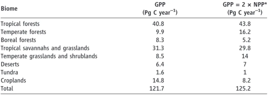
Tropical forests assimilate 34% of the global terrestrial GPP (Table 1) and have the highest GPP per unit area (table S5). Savannahs account for 26% of the global GPP and are the second most important biome in terms of global GPP. The large area of savannahs (about twice the sur-face area of tropical forests) explain their high contribution. Moreover, the results highlight the importance of taking into account C4 vegetation in global GPP estimates. Based on the C4 distribution (figs. S6 and S7), more than 20% of terrestrial GPP is conducted by C4 vegetation. Given that there were less than 20 site-years of flux data for C4-dominated ecosystems, our uncertainty is largest for this type of vegetation. Therefore, an expansion of observational net-works should focus on tropical C4 ecosystems. Boreal forests show a clear longitudinal gradient in GPP in northern Eurasia where GPP in the boreal zone decreases toward the east, where Table 1. GPP for biomes of the world as defined by Prentice et al. (6). Combining the biome extent (fig.
S17) with the spatially explicit GPP distributions by the approaches MTE1, MTE2, ANN, LUE, WUE, and KGB led to the respective median GPP per unit area separately for each biome (fig. S4). These medians were then multiplied by the biome area (6, 7) (fig. S4) to estimate GPP in column 2. The estimated GPP total of 122 Pg C year−1does not equal our overall median of 123 Pg C year−1because the biome area defined by fig. S17 and by (6) differ slightly. The third column shows GPP as estimated by using NPP numbers from Saugieret al. (7) under the assumption that NPP/GPP = 0.5 (6).
Biome GPP (Pg C year–1) GPP = 2 × NPP* (Pg C year–1) Tropical forests 40.8 43.8 Temperate forests 9.9 16.2 Boreal forests 8.3 5.2
Tropical savannahs and grasslands 31.3 29.8 Temperate grasslands and shrublands 8.5 14
Deserts 6.4 7
Tundra 1.6 1
Croplands 14.8 8.2
Total 121.7 125.2
*Based on integrated numbers for biomes (6, 7)
Fig. 2. Partial correla-tion in the spatial do-main between GPP from Fig. 1B and either (A) CRU precipitation, (B) CRU air temperature, or (C) ECMWF ERA-Interim short-wave radiation af-ter applying a moving 4.5° by 4.5° spatial win-dow and subsequent median filtering. Shown are significant
correla-Partial correlation median GPP and air temperature
−1 −0.5 0 0.5 1
Partial correlation median GPP and short−wave radiation
−1 −0.5 0 0.5 1 Partial correlation median GPP and precipitation
−1 −0.5 0 0.5 1 A B C tions (P < 0.01) of which the correlation coefficient is higher/lower than T 0.2.
on October 16, 2019
http://science.sciencemag.org/
photosynthesis is subject to an increasingly continental climate (Fig. 1B).
The latitudinal pattern derived by the different diagnostic models falls into a quite narrow range (Fig. 1C). In contrast, there is a larger range among an ensemble of five process-oriented biosphere models (Fig. 1C); in comparison to our data-oriented range, some consistently overestimate GPP, and others underestimate tropical GPP while matching or slightly overestimating GPP in the temperate zone (fig. S26). A standard global parametrization of the process-oriented models has been applied in this study; it was not optimized against flux tower GPP because we aimed at evaluating the process-based GPP fields and their correlations to climatic variables. For comparison, we show results by an additional, completely different approach of scaling GPP from flux tower sites to the regional scale (fig. S16), where a reationship between the sea-sonal NEE amplitude and annual GPP is derived at flux tower sites and applied to the seasonal NEE amplitude derived through atmospheric in-version [update of (33)]. This approach leads to values at the upper end of the range of the diag-nostic bottom-up approaches in northern extra-tropical regions but is still at the lower end of the range estimated by the process-oriented models. The differences between process-oriented and data-oriented estimates could lie in human-induced
degradation of GPP by land use (34). However, other reasons are possible, including insufficient model parametrization or structural model errors that lead to an overestimation of GPP.
Partial correlation analyses between GPP and climatic variables for 4.5° by 4.5° moving win-dows show that spatial variation of GPP is as-sociated with precipitation in 50 to 70% of the area of nontundra herbaceous ecosystems (Fig. 2A and Table 2). Also, 50% of the crop pro-duction occurs in regions where photosynthesis is colimited by precipitation, stressing the impor-tance of water availability for food security. Inter-estingly, GPP in the same proportion of temperate forest areas correlates positively with precipitation (Table 2). In contrast, the spatial GPP variability in only 30% of tropical and boreal forests seems to be associated positively with precipitation, but GPP of more than half of the boreal forests correlates positively with air temperature (Table 2). Therefore, the GPP of these biomes seems to be robust against a moderate climate variation in the order of magnitude of the current spatial var-iability of climate, given the very low probability of a decrease in air temperature in the boreal zone. We find negative correlations of productivity with incoming short-wave radiation, in particular in savannahs, the Mediterranean, and Central Asian grasslands (Fig. 2C and tables S6 to S8).
These negative partial correlations may indicate an additional indirect effect of radiation or tem-perature on GPP by the water balance. Both cli-matic variables are usually associated with higher evapotranspiration rates, which will yield more negative water balances with higher temperature or radiation levels with consequent negative effects on primary productivity in these water-limited re-gions. This interpretation is possible notwithstanding a direct effect of temperature on vegetation by heat stress as well as increased levels of diffuse radiation associated with overall lower levels of radiation (35).
After four decades of research on the global magnitude of primary production of terrestrial vegetation (23, 36), we present an observation-based estimate of global terrestrial GPP. Although we arrive at a global GPP of similar magnitude as these earlier estimates, our results add confidence and spatial details. The large range of GPP results by process-oriented biosphere models indicates the need for further constraining CO2uptake
pro-cesses in these models. Furthermore, our spatially explicit GPP results contribute to a quantification of the climatic control of GPP. Complementing theoretical or process-oriented results (37, 38) about climatic limitations of GPP, our observation-based results now constitute empirical evidence for a large effect of water availability on primary production over 40% of the vegetated land (Fig. 3A) and up to 70% in savannahs, shrublands, grass-lands, and agricultural areas (Table 2). Our find-ings imply a high susceptibility of these ecosystems’ productivity to projected changes of precipitation over the 21st century (39), but a robustness of tropical and boreal forests. Results of current pro-cess models show a large range and a tendency to overestimate precipitation-associated GPP (Fig. 3B). Most likely, the association of GPP and cli-mate in process-oriented models can be improved by including negative feedback mechanisms (e.g., adaptation) that might stabilize the systems. Our high spatial resolution GPP estimates, their uncer-tainty, and their relationship to climate drivers should be useful for evaluating and thus improving coupled climate–carbon cycle process models. Fig. 3. Percentage of vegetated land
surface (A) and corresponding GPP (B) that is controlled by precipitation, de-pending on the chosen threshold for the partial correlation coefficients that signal a control of GPP by a climate fac-tor. The blue areas represent the range of data-driven estimates (MTE1, MTE2, ANN, LUE, and KGB) using different cli-mate sources [CRU, ECMWF ERA-Interim, and GPCP (16)]. This is compared to the range of process-oriented model results (LPJ-DGVM, LPJmL, ORCHIDEE, CLM-CN, and SDGVM) in red. Purple shows the overlapping area. The thick lines repre-sent the medians of both ranges. For
instance, GPP of about 40% of the vegetated land surface is controlled by water availability by defining a water control of GPP as a partial correlation coefficient between GPP and precipitation higher than 0.2.
Table 2. Percentage of biome area for which GPP is climatically controlled, indicated by a median partial correlation coefficient higher than 0.2 (or 0.5 in brackets). Several climate grids (CRU, ECMWF ERA-Interim, and GPCP precipitation) were used to perform a partial correlation between the median GPP map (Fig. 1B) and climate variables for 4.5° by 4.5° moving windows (16). Then, the fractional area with significant (P < 0.01) partial correlation higher than 0.2 (0.5) was calculated.
Biome P* controlled T† controlled R‡ controlled Tropical forests 29 (12) 39 (26) 4 (1) Temperate forests 50 (26) 41 (23) 6 (2)
Boreal forests 20 (5) 55 (31) 21 (7)
Tropical savannahs and grasslands 55 (31) 16 (5) 3 (0) Temperate grasslands and shrublands 69 (41) 37 (18) 6 (1)
Deserts 61 (37) 18 (6) 8 (2)
Tundra 24 (13) 37 (27) 32 (12)
Croplands 51 (25) 28 (13) 5 (1)
*Precipitation †Air temperature ‡Short-wave radiation
on October 16, 2019
http://science.sciencemag.org/
References and Notes
1. E.-D. Schulze, Flora 159, 177 (1970).
2. H. Poorter, C. Remkes, H. Lambers, Plant Physiol. 94, 621 (1990).
3. E. H. DeLucia, J. E. Drake, R. B. Thomas, M. Gonzalez-Meler, Glob. Change Biol. 13, 1157 (2007).
4. S. Luyssaert et al., Glob. Change Biol. 13, 2509 (2007). 5. C. M. Litton, J. W. Raich, M. G. Ryan, Glob. Change Biol.
13, 2089 (2007).
6. I. C. Prentice et al., Climate Change 2001: The Scientific Basis. Contribution of Working Group I to the Third Assessment Report of the Intergovernmental Panel on Climate Change, J. Houghton, et al., Eds. (Cambridge
University Press, Cambridge, 2001), pp. 183–237.
7. B. Saugier, J. Roy, H. A. Mooney, Terrestrial Global Productivity, J. Roy, B. Saugier, H. A. Mooney, Eds. (Academic Press, San Diego, CA, 2001). 8. G. D. Farquhar et al., Nature 363, 439 (1993). 9. P. Ciais et al., J. Geophys. Res. 102 (D5), 5857 (1997). 10. L. Wingate et al., Proc. Natl. Acad. Sci. U.S.A. 106,
22411 (2009).
11. L. Sandoval-Soto et al., Biogeosciences 2, 125 (2005). 12. J. E. Campbell et al., Science 322, 1085 (2008). 13. P. Suntharalingam, A. J. Kettle, S. M. Montzka,
D. J. Jacob, Geophys. Res. Lett. 35, L19801 (2008). 14. P. Friedlingstein et al., J. Clim. 19, 3337 (2006). 15. D. Baldocchi, Aust. J. Bot. 56, 1 (2008). 16. Materials and methods are available as supporting
material on Science Online.
17. M. Jung, M. Reichstein, A. Bondeau, Biogeosciences 6, 2001 (2009).
18. D. Papale, R. Valentini, Glob. Change Biol. 9, 525 (2003). 19. C. Beer, M. Reichstein, P. Ciais, G. D. Farquhar,
D. Papale, Geophys. Res. Lett. 34, L05401 (2007). 20. C. Beer et al., Glob. Biogeochem. Cycles 23, GB2018 (2009). 21. J. Monteith, J. Appl. Ecol. 9, 747 (1972).
22. S. W. Running, P. Thornton, R. Nemani, J. Glassy, Methods in Ecosystem Science, O. Sala, R. Jackson, H. Mooney, R. Howarth,
Eds. (Springer-Verlag, New York, 2000), pp. 44–57.
23. H. Lieth, Primary Productivity of the Biosphere, H. Lieth, R. H. Whittaker, Eds. (Springer-Verlag, Berlin, 1975),
pp. 237–263.
24. R. Myneni et al., Remote Sens. Environ. 83, 214 (2002). 25. N. Gobron et al., J. Geophys. Res.-Atmos. 111 (D13),
D13110 (2006).
26. F. Baret et al., Remote Sens. Environ. 110, 275 (2007). 27. M. New, D. Lister, M. Hulme, I. Makin, Clim. Res. 21,
1 (2002).
28. T. D. Mitchell, P. D. Jones, Int. J. Climatol. 25, 693 (2005). 29. A. Simmons, S. Uppala, D. Dee, S. Kobayashi, ECMWF
Newsletter No. 110 (European Centre for Medium-Range Weather Forecasts, Shinfield Park, Reading, UK, 2007). 30. Median absolute deviation times 1.48.
31. B. Fekete, C. Vorosmarty, J. Roads, C. Willmott, J. Clim. 17, 294 (2004).
32. M. Zhao, S. W. Running, R. R. Nemani, J. Geophys. Res.-Biogeosci. 111 (G1), G01002 (2006). 33. C. Rödenbeck, S. Houweling, M. Gloor, M. Heimann,
Atmos. Chem. Phys. 3, 1919 (2003).
34. A. Bondeau et al., Glob. Change Biol. 13, 679 (2007). 35. L. M. Mercado et al., Nature 458, 1014 (2009). 36. R. H. Whittaker, G. E. Likens, Primary Productivity of the
Biosphere, H. Lieth, R. H. Whittaker, Eds.
(Springer-Verlag, Berlin, 1975), pp. 305–328.
37. R. R. Nemani et al., Science 300, 1560 (2003). 38. D. Gerten et al., Geophys. Res. Lett. 32, L21408 (2005). 39. G. Meehl et al., in Climate Change 2007: The Physical Science
Basis. Contribution of Working Group I to the Fourth Assessment Report of the Intergovernmental Panel on Climate Change, S. Solomon et al., Eds. (Cambridge University Press,
Cambridge and New York, 2007), pp. 747–845.
40. This work used eddy covariance data acquired by the FLUXNET community and in particular by the following networks: AmeriFlux [U.S. Department of Energy, Biological and Environmental Research, Terrestrial Carbon Program (DE-FG02-04ER63917 and DE-FG02-04ER63911)], AfriFlux, AsiaFlux, CarboAfrica, CarboEuropeIP, CarboItaly, CarboMont, ChinaFlux, Fluxnet-Canada (supported by CFCAS, NSERC, BIOCAP, Environment Canada, and NRCan), GreenGrass, KoFlux, LBA, NECC, OzFlux, TCOS-Siberia, and USCCC. We acknowledge the support to the eddy covariance data harmonization provided by CarboEuropeIP, FAO-GTOS-TCO, Integrated Land Ecosystem-Atmosphere Processes Study, Max
Planck Institute for Biogeochemistry, National Science Foundation, University of Tuscia, Université Laval and Environment Canada and U.S. Department of Energy and the database development and technical support from Berkeley Water Center, Lawrence Berkeley National Laboratory, Microsoft Research eScience, Oak Ridge National Laboratory,
University of California–Berkeley, and University of Virginia.
Remotely sensed land cover, fAPAR, and LAI were available through the Joint Research Centre of the European Commission, the National Aeronautics and Space Administration, and the projects GLC2000 and CYCLOPES. Climate data came from the European Centre for Medium-Range Weather Forecasts, the Climate Research Unit of the University of East Anglia, and the GEWEX project GPCP. We thank Mahendra K. Karki at GMAO/NASA for extracting the MOD17 required surface meteorological variables from the GMAO reanalysis dataset and Maosheng Zhao at NTSG of University of Montana for calculating the respective daytime VPD. We further acknowledge support by the European Commission FP7 projects COMBINE and CARBO-Extreme and a grant from the Max-Planck Society establishing the MPRG Biogeochemical Model-Data Integration. C.B., D.P., M.R., P.C., D.B., and S.L. conceived the study. C.B., C.R., D.P., E.T., M.J., M.R., and N.C. contributed diagnostic modeling results. C.B., A.B., G.B.B., M.L., F.I.W., and N.V. contributed process model results. C.B., E.T., and M.R. performed the analysis. C.B. and M.R. wrote the manuscript. All other coauthors contributed with data or substantial input to the manuscript.
Supporting Online Material
www.sciencemag.org/cgi/content/full/science.1184984/DC1 Materials and Methods
SOM Text Figs. S1 to S34 Tables S1 to S9 References
20 November 2009; accepted 8 June 2010 Published online 5 July 2010;
10.1126/science.1184984
Include this information when citing this paper.
Global Convergence in the
Temperature Sensitivity of Respiration
at Ecosystem Level
Miguel D. Mahecha,1,2* Markus Reichstein,1Nuno Carvalhais,1,3Gitta Lasslop,1Holger Lange,4 Sonia I. Seneviratne,2Rodrigo Vargas,5Christof Ammann,6M. Altaf Arain,7Alessandro Cescatti,8
Ivan A. Janssens,9Mirco Migliavacca,10Leonardo Montagnani,11,12Andrew D. Richardson13 The respiratory release of carbon dioxide (CO2) from the land surface is a major flux in the global carbon
cycle, antipodal to photosynthetic CO2uptake. Understanding the sensitivity of respiratory processes to
temperature is central for quantifying the climate–carbon cycle feedback. We approximated the sensitivity of terrestrial ecosystem respiration to air temperature (Q10) across 60 FLUXNET sites with the use of a
methodology that circumvents confounding effects. Contrary to previous findings, our results suggest that Q10is independent of mean annual temperature, does not differ among biomes, and is confined to values
around 1.4T 0.1. The strong relation between photosynthesis and respiration, by contrast, is highly variable among sites. The results may partly explain a less pronounced climate–carbon cycle feedback than suggested by current carbon cycle climate models.
Q
uantifying the intensity of feedback mechanisms between terrestrial ecosys-tems and climate is a central challenge for understanding the global carbon cycle and a prerequisite for reliable future climate sce-narios (1, 2). One crucial determinant of the climate–carbon cycle feedback is the temperature sensitivity of respiratory processes in terrestrial ecosystems (3, 4), which has been subject tomuch debate (5–10). On the one hand, empirical studies have found high sensitivities of soil respiration to temperature, with values of Q10
(here an indicator of the sensitivity of terrestrial ecosystem respiration to air temperature) well above 2 (11, 12). Dependencies of Q10values on
mean temperatures (12, 13) have been attributed to the acclimatization of soil respiration (5), among other factors (13). On the other hand, global-scale
models often make use of globally constantQ10
values of 2 or below to generate carbon dynamics consistent with global atmospheric CO2 growth
rates (3, 14, 15). Nonetheless, several models have directly included empirical dependencies of the parameterization of respiratory processes to envi-ronmental dynamics (16–18). This inclusion is questionable, given that single-site studies have in-dicated that factors seasonally covarying with tem-perature can confound the experimental retrieval
1
Max Planck Institute for Biogeochemistry, 07745 Jena, Germany. 2
Institute for Atmospheric and Climate Science, ETH Zürich, Universitätsstrasse 16, 8092 Zürich, Switzerland.3Faculdade de Ciências e Tecnologia, FCT, Universidade Nova de Lisboa, 2829-516 Caparica, Portugal.4Norsk Institutt for Skog og Landskap, N-1431 A˚s, Norway.5Department of Environmental Science, Policy and Management, University of California, Berkeley, CA 94720, USA. 6
Agroscope ART, Federal Research Station, Reckenholzstr. 191, CH-8046 Zürich, Switzerland.7McMaster Centre for Climate Change, McMaster University, Hamilton, Ontario L8S 4L8, Canada.8 Euro-pean Commission, Joint Research Center, Institute for Environment and Sustainability, I-21027 Ispra, Italy.9Department of Biology, University of Antwerpen, Universiteitsplein 1, 2610 Wilrijk, Belgium. 10
Remote Sensing of Environmental Dynamics Laboratory, DISAT, University of Milano-Bicocca, 20126 Milano, Italy.11Servizi Forestali, Agenzia per l’Ambiente, Provincia Autonoma di Bolzano, 39100 Bolzano, Italy.12Faculty of Sciences and Technologies, Free Uni-versity of Bozen-Bolzano, Piazza Università 1, 39100 Bolzano, Italy. 13Harvard University Department of Organismic and Evolutionary Biology, Harvard University Herbaria, 22 Divinity Avenue, Cambridge, MA 02138, USA.
*To whom correspondence should be addressed. E-mail: mmahecha@bgc-jena.mpg.de
on October 16, 2019
http://science.sciencemag.org/
Christopher Williams, F. Ian Woodward and Dario Papale
Lomas, Sebastiaan Luyssaert, Hank Margolis, Keith W. Oleson, Olivier Roupsard, Elmar Veenendaal, Nicolas Viovy, Altaf Arain, Dennis Baldocchi, Gordon B. Bonan, Alberte Bondeau, Alessandro Cescatti, Gitta Lasslop, Anders Lindroth, Mark Christian Beer, Markus Reichstein, Enrico Tomelleri, Philippe Ciais, Martin Jung, Nuno Carvalhais, Christian Rödenbeck, M.
originally published online July 5, 2010 DOI: 10.1126/science.1184984
(5993), 834-838. 329
Science
recent climate models.
level of temperature sensitivity suggests a less-pronounced climate sensitivity of the carbon cycle than assumed by to mean annual temperature, independent of the analyzed ecosystem type, with a global mean value for Q10 of 1.6. This
(p. 838, published online 5 July) now show that the Q10 of ecosystem respiration is invariant with respect
et al.
Mahecha
of ecosystem respiratory processes is a key determinant of the interaction between climate and the carbon cycle. forests, and precipitation controls carbon uptake in more than 40% of vegetated land. The temperature sensitivity (Q10) comparison, burning fossil fuels emits about 7 billion tons annually. Thirty-two percent of this uptake occurs in tropical observation and calculation to estimate that the total GPP by terrestrial plants is around 122 billion tons per year; in
(p. 834, published online 5 July) used a combination of
et al.
Beer atmosphere every year to fuel photosynthesis.
removed from the 2
). Gross primary production (GPP) is a measure of the amount of CO Reich
the Perspective by
As climate change accelerates, it is important to know the likely impact of climate change on the carbon cycle (see Carbon Cycle and Climate Change
ARTICLE TOOLS http://science.sciencemag.org/content/329/5993/834
MATERIALS SUPPLEMENTARY http://science.sciencemag.org/content/suppl/2010/07/01/science.1184984.DC1 CONTENT RELATED file:/contentpending:yes http://science.sciencemag.org/content/sci/329/5993/838.full http://science.sciencemag.org/content/sci/329/5993/774.full http://science.sciencemag.org/content/sci/330/6010/1476.3.full REFERENCES http://science.sciencemag.org/content/329/5993/834#BIBL
This article cites 30 articles, 4 of which you can access for free
PERMISSIONS http://www.sciencemag.org/help/reprints-and-permissions
Terms of Service
Use of this article is subject to the
is a registered trademark of AAAS. Science
Science, 1200 New York Avenue NW, Washington, DC 20005. The title
(print ISSN 0036-8075; online ISSN 1095-9203) is published by the American Association for the Advancement of Science
Copyright © 2010, American Association for the Advancement of Science
on October 16, 2019
http://science.sciencemag.org/