The Achievable Region Method in the Optimal Control of Queueing Systems; Formulations,
Bounds and Policies
Dimitris Bertsimas
The achievable region method in the optimal control of queueing
systems; formulations, bounds and policies
Dimitris Bertsimas
Sloan School of Management and Operations Research Center
Massachusetts Institute of Technology, E53-359
Cambridge, MA 02139
Revised June 1995
Abstract
We survey a new approach that the author and his co-workers have developed to formulate stochastic control problems (predominantly queueing systems) as mathematical programming
prob-lems. The central idea is to characterize the region of achievable performance in a stochastic control
problem, i.e., find linear or nonlinear constraints on the performance vectors that all policies satisfy. We present linear and nonlinear relaxations of the performance space for the following problems: In-dexable systems (multiclass single station queues and multiarmed bandit problems), restless bandit problems, polling systems, multiclass queueing and loss networks. These relaxations lead to bounds on the performance of an optimal policy. Using information from the relaxations we construct heuris-tic nearly optimal policies. The theme in the paper is the thesis that better formulations lead to deeper understanding and better solution methods. Overall the proposed approach for stochastic control problems parallels efforts of the mathematical programming community in the last twenty years to develop sharper formulations (polyhedral combinatorics and more recently nonlinear relax-ations) and leads to new insights ranging from a complete characterization and new algorithms for indexable systems to tight lower bounds and nearly optimal algorithms for restless bandit problems, polling systems, multiclass queueing and loss networks.
Keywords: Queueing networks, loss networks, multiarmed bandits, bounds, policies, opti-mization.
1
Introduction
In its thirty-years history the area of optimal control of stochastic systems (predominantly queueing systems) has addressed with various degrees of success several key problems that arise in areas as diverse as computer and communication networks, manufacturing and service systems. A general characteristic of this body of research is the lack of a unified method of attack for these problems. Every problem seems to require its own formulation and, as a result, its own somewhat ad hoc approach. Moreover, quite often it is not clear how close a proposed solution is to the optimal solution.
In contrast, the field of mathematical programming has evolved around a very small collection of key problem formulations: network, linear, integer and nonlinear programs. In this tradition, researchers and practitioners solve optimization problems by defining decision variables and formulating constraints, thus describing the feasible space of decisions, and applying algorithms for the solution of the underlying optimization problem. When faced with a new deterministic optimization problem, researchers and practitioners have indeed an a priori well-defined plan of attack to solve it: model it as a network, linear, integer or nonlinear program and then use a well-established algorithm for its solution. In this way they obtain feasible solutions which are either provably optimal or with a guarantee for the degree of their suboptimality.
Our goal in this paper is to review an approach to formulate stochastic control problems (predom-inantly queueing systems) as mathematical programming problems. In this way we are able to produce bounds on the performance of an optimal policy and develop optimal or near-optimal policies using in-formation from the formulations. We address the following problems, which, are, in our opinion, among the most important in applications and among the richest in modeling power and structure (detailed definitions of the problems are included in the corresponding sections of the paper):
1. Indexable systems (multiclass queues and multiarmed bandit problems). 2. Restless bandit problems.
3. Polling systems.
4. Multiclass queueing networks. 5. Multiclass loss networks.
In order to motivate the approach we first comment on the power of formulations in mathematical optimization, then describe the approach of the paper in stochastic control in broad terms and put it in a historical perspective.
On the power of formulations in mathematical optimization
Our ability to solve efficiently mathematical optimization problems is to a large degree proportional to our ability to formulate them. In particular, if we can formulate a problem as a linear optimization
and exponential number of constraints such that we can solve the separation problem in polynomial time) we can solve the problem efficiently (in polynomial time). On the other hand, the general integer
optimization problem (IP) is rather difficult (the problem is AP-hard). Despite its hardness, the
mathe-matical programming community has developed methods to successfully solve large scale instances. The central idea in this development has been improved formulations. Over the last twenty years much of the effort in integer programming research has been in developing sharper formulations using polyhedral methods and more recently techniques from semidefinite optimization (see for example LovAsz and Schri-jver [391). Given that linear programming relaxations provide bounds for IP, it is desirable to enhance the formulation of an IP by adding valid inequalities, such that the relaxation is closer and closer to the IP. We outline the idea of improved formulations in the context of IP in Figure la.
On the power of formulations in stochastic control
Motivated by the power of improved formulations for mathematical programming problems, we shall now outline in broad terms the approach taken in this paper to formulate stochastic control problems as
mathematical programming problems. The key idea is the following: Given a stochastic control problem,
we define a vector of performance measures (these are typically expectations, but not necessarily first moments) and then we express the objective function as a function of this vector. The critical idea is to characterize the region of achievable performance (or performance space), i.e., find constraints on the performance vectors that all policies satisfy. In this way we find a series of relaxations that are progressively closer to the exact region of achievable performance. In Figure lb we outline the conceptual similarity of this approach to the approach used in integer programming. Interestingly we will see that we can propose both linear and nonlinear relaxations (the latter also based on ideas from semidefinite programming).
The idea of describing the performance space of a queueing control problem has its origin in the work of Coffman and Mitrani [15] and Gelenbe and Mitrani [20], who first showed that the performance space of a multiclass M/G/1 queue under the average-cost criterion can be described as a polyhedron. Federgruen and Groenevelt [18], [19] advanced the theory further by observing that in certain special cases of multiclass queues, the polyhedron has a very special structure (it is a polymatroid) that gives rise to very simple optimal policies (the c/p rule). Their results partially extend to some rather restricted multiclass queueing networks, in which it is assumed that all classes of customers have the same routing probabilities, and the same service requirements at each station of the network (see Ross and Yao [47]). Shanthikumar and Yao [50] generalized the theory further by observing that if a system satisfies certain
work conservation laws, then the underlying performance space is necessarily a polymatroid. They also
proved that, when the cost is linear on the performance, the optimal policy is a static priority rule (Cox and Smith [16]). Tsoucas [57] derived the region of achievable performance in the problem of scheduling a multiclass nonpreemptive M/G/1 queue with Bernoulli feedback, introduced by Klimov [35].
stochas-veu ition I 1 X1 Exact formulation Convex Hull (a) Nonlinear LP relaxation Relaxation
x,
1
1
Exact Formulation (b) A-Figure 1: (a) Improved relaxations for integer programming (b) Improved relaxations for stochastic optimization problems.
tic control problems that include all the previous queueing control and multiarmed bandit problems, establishing that the strong structural properties for these problems follow from the corresponding prop-erties of the underlying polyhedra. Interestingly this exact characterization of the achievable region as a polyhedron leads to an exact algorithm that uses linear programming duality and naturally defines indices (Gittins indices) as dual variables. We review these developments in Section 2.
For restless bandit problems Whittle [62] proposes a relaxation that provides a bound for the problem. Bertsimas and Nifio-Mora [7] propose a series of increasing more complicated relaxations (the last one being exact) that give increasingly stronger bounds and a heuristic that naturally arises from these relaxations using duality that empirically gives solutions which are close to the optimal one. We review these developments in Section 3.
For polling systems Bertsimas and Xu [10] propose a nonlinear (but convex) relaxation, and a heuristic that uses integer programming techniques, that provides near optimal static policies. We review these developments in Section 4.
For queueing network problems Bertsimas, Paschalidis and Tsitsiklis [8] propose a linear programming relaxation that provides bounds for the optimal solution using a systematic method to generate linear constraints on the achievable region. In this paper we propose stronger nonlinear relaxations that are based on ideas from semidefinite programming. We review these developments in Section 5.
For loss networks Kelly [33] has developed bounds based on nonlinear optimization, while Bertsimas and Crissikou [5] propose a series of increasingly more complex linear relaxations (the last one being
X2
I I
- - |
I .-.j Z
W-exact) and a heuristic that arises from these relaxations. We review these developments in Section 6. In Section 7 we present some theoretical limitations of the current approach using some negative complexity results, while in Section 8 we conclude with some open problems.
2
Indexable systems
Perhaps one of the most important successes in the area of stochastic control in the last twenty years is the solution of the celebrated multiarmed bandit problem, a generic version of which in discrete time is as follows:
The multiarmed bandit problem: There are K parallel projects, indexed k = 1,..., K. Project
k can be in one of a finite number of states jk E Ek. At each instant of discrete time t = 0, 1,...
one can work only on a single project. If one works on project k in state jk(t) at time t, then one receives an immediate reward of Rkj,(t). Rewards are additive and discounted in time by a discount factor 0 < < 1. The state jk(t) changes to jk(t + 1) by a homogeneous Markov transition rule, with transition matrix pk = (p)ijEEk, while the states of the projects one has not engaged remain frozen. The problem is how to allocate one's resources to projects sequentially in time in order to maximize expected total discounted reward over an infinite horizon. More precisely, one chooses a policy u (among a set of policies U) for specifying the project k(t) to work on at each point of time t to achieve:
max Eu tIkt= k
uEU
[
The problem has numerous applications and a rather vast literature (see Gittins [23] and the references therein). It was originally solved by Gittins and Jones [21], who proved that to each project k one could attach an index yk'(jk(t)), which is a function of the project k and the current state jk(t) alone, such
that the optimal action at time t is to engage a project of largest current index. They also proved the important result that these index functions satisfy a stronger index decomposition property: the function yk(.) only depends on characteristics of project k (states, rewards and transition probabilities), and not on any other project. These indices are now known as Gittins indices, in recognition of Gittins contribution. Since the original solution, which relied on an interchange argument, other proofs were proposed: Whittle [61] provided a proof based on dynamic programming, subsequently simplified by Tsitsiklis [55]. Varaiya, Walrand and Buyukkoc [58] and Weiss [60] provided different proofs based on interchange arguments. Weber [59] and Tsitsiklis [56] outlined intuitive proofs.
The multiarmed bandit problem is a special case of a stochastic service system S. In this context, there is a finite set E of job types. Jobs have to be scheduled for service in the system. We are interested in optimizing a function of a performance measure (rewards or taxes) under a class of admissible scheduling policies. A policy is called admissible if the decision as to which project to operate at any time t must be based only on information on the current states of the projects.
Definition 1 (Indexable Systems) We say that a stochastic serice system S is indexable if the
fol-lowing policy is optimal: to each job type i we attach an index yi. At each decision epoch select a job with largest current index.
In general the optimal indices Yi (as functions of the parameters of the system) could depend on charac-teristics of the entire set E of job types. Consider a partition of set E into subsets Ek, for k = 1,..., K. Job types in subset Ek can be interpreted as being part of a common project type k. In certain situa-tions, the optimal indices of job types in Ek depend only on characteristics of job types in Ek and not on the entire set E. Such a property is particularly useful computationally since it enables the system to be decomposed into smaller components and the computation of the indices for each component can be done independently. As we have seen the multiarmed bandit problem has this decomposition property, which motivates the following definition:
Definition 2 (Decomposable Systems) An indexable system is called decomposable if for all job
types i E Ek, the optimal index yi of job type i depends only on characteristics of job types in Ek. In addition to the multiarmed bandit problem, a variety of stochastic control problems has been solved in the last decades by indexing rules (see Table 3 for examples).
Faced with these results, one asks what is the underlying reason that these nontrivial problems have very efficient solutions both theoretically as well as practically. In particular, what is the class of
stochas-tic control problems that are indexable? Under what conditions are indexable systems decomposable? But
most importantly, is there a unified way to address stochastic control problems that will lead to a deeper
understanding of their structural properties?
In this section we review the work of Bertsimas and Nifio-Mora [6]. In Section 2.1 we introduce via an example of a multiclass queue with feedback, which is a special case of the multiarmed bandit problem, the idea of work conservation laws. These physical laws of the system constrain the region of achievable performance and imply that it is a polyhedron of special structure called extended contra-polymatroid. In this way the stochastic control problem can be reduced to a linear programming problem over this polyhedron. In Section 2.2 we propose an efficient algorithm to solve the linear programming problem and observe that the algorithm naturally defines indices. In Sections 2.3 we consider examples of natural problems that can be analyzed using the theory developed, while in Section 2.4 we outline implications of these characterizations.
2.1 Work conservation laws
In order to present the idea of conservation laws we consider the so called Klimov problem with n = 3 classes: three Poisson arrival streams with rates Ai arrive at a single server. Each class has a different service distribution. After service completion, a job of class i becomes a job of class j with probability
Pij and leaves the system with probability 1 - k ik. Let xz be the expected queue length of class i under policy u. What is the space of vectors (xz', x, xu) as the policies u vary? For every policy
Ai') "2' > b({i}) i = 1, 2,3
which means that the total work class i brings to the system under any policy is at least as much as the work under the policy that gives priority to class i. Similarly, for every subset of classes, the total work that this set of classes brings to the system under any policy is at least as much as the work under the policy that gives priority to this set of classes:
A?'212l + A1,'21
22 > b({1,2}), A1,3}1 X+ A{1'3} 3 > b({1, 3}),
A{2,32 + A 2'3 x3 > b({2, 3}).
Finally, there is work conservation, i.e., all nonidling policies require the same total work: A1,2,3 ,2,3 + + A1,2,31 +3 = b({1,2, 3}).
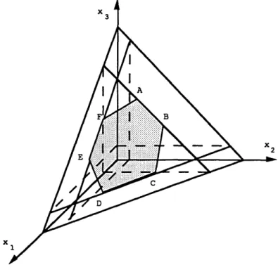
The performance space in this example consists exactly of the 23- 1 = 7 constraints. In Figure 2 we present the performance space for this example.
Figure 2: An extended contra-polymatroid in dimension 3.
The polytope has 3! = 6 extreme points corresponding to the 6 permutations of a set of 3 elements. Extreme point A corresponds to the performance vector of the policy that gives highest priority to class
1, then to class 2 and last priority to class 3. The vector corresponding to point A is the unique solution of the triangular system:
A1'X2 1 =1,21
A'12}l 1+ A{12} 2 = b({1, 2}),
A {1,2,31X + A{1'2,3 Z2+ A1,2,3 3 = b({1, 2, 3}).
Polyhedra of this type are called extended contra-polymatroids and have the property that their extreme points correspond to the performance vectors of complete priority policies.
In order to present these ideas more generally we consider next a generic stochastic seruice system. There are n job types, which we label i E E = {1,..., n}. Jobs have to be scheduled for service in the
system. Let us denote U the class of admissible scheduling policies. Let xz' be a performance measure of type i jobs under admissible policy u, for i E E. We assume that x' is an expectation. Let x, denote the performance vector under a static priority rule (i.e., the servicing priority of a job does not change over time) that assigns priorities to the job types according to permutation 7r = (rl,..., irn) of E, where type rn has the highest priority.
Definition 3 (Conservation Laws) The performance vector x is said to satisfy conservation laws if
there exist a set function b(-) :2E --. A+ and a matrix A = (AS)iEE,SCE satisfying
As > 0, for iES and A = 0, for i E S, for all S C E, such that:
(a)
b(S) = A i
x
for all 7r: {rl,r.. .,rSrl1} = S and SC E; (1)iES
(b) For all admissible policies u E U,
Z
ASxu > b(S) for all S C E and E AEx.u = b(E), (2)iES iEE
or respectively,
Z
ASxu < b(S) for all S C E and E AxI' = b(E). (3)iES iE
Condition (1) means that all policies which give priority to the set E \ S over the set S have the same performance irrespective of the rule used within S or within E \ S. Moreover, all such policies have the same performance b(S) (conservation law). Condition (2) means that all other policies have performance bigger than b(S), while for S = E all policies have the same performance.
The following theorem characterizes the performance space for a performance vector x satisfying conservation laws as a polyhedron.
Theorem 1 Assume that performance vector x satisfies conservation laws (1) and (2) (respectively (1) and (3)). Then
(a) The performance space for the vector x is exactly the polyhedron
c(A,b)= {xE I A:ASzi > b(S), forSC E and ZAE xi b(E)), (4)
iES iEE
or respectively
B(A, b) = x E Rn+: ASxi < b(S), for SC E and Z AExi b(E)}. (5)
iES iEE
(b) The vertices of Bc(A, b) (respectively B(A,b)) are the performance vectors of the static priority rules.
We can explicitly characterize the performance vectors corresponding to priority rules as follows. Let 7r = (7r1, .. .,Tr) be a permutation of E corresponding to the static priority rule 7r. We let x, =
(xrl ... X, )' be the performance vector corresponding to the static priority rule r. We also let
bar
=
(b((7rl), b(I-7r, lr2)), ... , b(f{rl, . , 7rn))'.Let A, denote the following lower triangular submatrix of A:
A{w ,2} AIl2} ) 0
A, = I.
r, A WX2 · * Xn
Then, the performance vector x, is the unique solution of the linear system
A{il.rj}x, = b({7ri, 7rj}), j=1,...,n (6)
i=1
or, in matrix notation:
x = A'lb,. (7)
It is not obvious that the vector x, E B3(A, b) found in (7). This is a consequence of the fact that the performance vectors satisfy conservation laws. This motivates the following definition based on Bhattacharya et. al. [12]:
Definition 4 (Extended Polymatroid) We say that polyhedron B(A, b) is an extended polymatroid with ground set E and correspondingly B3(A, b) is an extended contra-polymatroid if for every permu-tation 7r of E, x7, E B(A, b) or correspondingly x, E B3(A, b).
The connection of conservation laws and extended polymatroids is that if a performance vector x satisfies conservation laws (1) and (2) (resp. (1) and (3)), then its performance space B3(A,b) in (4) (resp. B(A, b) in (5)) is an extended polymatroid (resp. contra-polymatroid).
Remark: If As = 1 for all i E S, x, E B(A, b) if and only if the set function b(S) is submodular, i.e., for all S, T C E,
b(S) + b(T) < b(S n T) + b(S u T).
This case corresponds to the usual polymatroids introduced in Edmonds [17].
2.2 An algorithm for optimization of indexable systems
Suppose that we want to find an admissible policy u E U that maximizes a linear reward function on the performance RtEE Rixi', where the vector x satisfies conservation laws (1) and (2). This optimal
control problem can be expressed as
(LPu) max Ri4: u EU}. (8)
iEE
By Theorem 1 this optimal control problem can be transformed into the following linear programming problem over an extended contra-polymatroid.
(LPc) max Rii: x E Bc(A, b) (9)
iEE
The theory over extended polymatroids is completely analogous. Given that the extreme points of the polytope B3(A, b) correspond to priorities (permutations), the problem reduces to finding which priority is optimal.
Tsoucas [57] and Bertsimas and Nifio-Mora [6] presented the following adaptive greedy algorithm. The algorithm constructs an optimal solution y to the linear programming dual of problem (LPc). It first decides, which class will have the highest priority 7rn by calculating the maximum , i E E (this is the greedy part of the algorithm). This value is assigned to x,,. It then modifies the rewards (this is the adaptive part of the algorithm) and picks the next class by performing a similar maximum ratio test. The algorithm also calculates numbers yi, which define indices. We next formally present the algorithm.
Algorithm A5
Input: (R, A).
Output: (-y, 7r, y,,,S), where r = (r,.. .,7rn) is a permutation of E, y = yS)sCE v = (v1 I n), and S = S,...,Sn}, with Sk = 7rl,..., 7rk, for k E E.
Step 0. Set Sn = E. Set = max{ : i E E }; pick 7rn E argmax{ R.: i E E };
set y,, = v,.
Step k. For k 1, ... , n- 1:
Ri-\`I-I Zl
Set Sn-k = Sn-k+l \ 7{rn-k+l }; set vn-k = max{ -j=: i E S-n-k }; A~._. A~.
pick 7rnk E argmax{ nk n--k } Ai=
V-k-Problem Feasible space Indices Optimal solution E
ZEs Asxi > b(S), SC E
(LP) minXEs(Ab) Cx (A, b) : iEE AxEi = b(E) (C, A) Ay 7 _ |y , < < <r,y x>_
aExtended polymatroid bExtended contra-polymatroid
Step n. For S C E set
j, if S = Sj for some j E E;
Bertsimas and Niiio-Mora [6] show that outputs 7y and y of algorithm AG are uniquely determined by the input (R, A). Moreover, y is an optimal solution to the linear programming dual of (LPc). The above algorithm runs in O(n3). They also show, using linear programming duality, that linear program (LPc) has the following indexability property.
Definition 5 (Generalized Gittins Indices) Let y be the optimal dual solution generated by algo-rithm Ag. Let
'v= E Sw iEE.
S: EDS3i
We say that
-y,
... , My, are the generalized Gittins indices of linear program (LPc).Theorem 2 (Indexability of LP over extended polymatroids) Linear program (LPc) is optimized
by the vector x, where r is any permutation of E such that
rt -< '< A, (10)
Let yl, ... , be the generalized Gittins indices of linear program (LPc). A direct consequence of-7n the previous discussion is that the control problem (LPu) is solved by an index policy, with indices given by 71y,.... ,n.
Theorem 3 (Indexability of Systems Satisfying Conservation Laws) A policy that selects at each decision epoch a job of currently largest generalized Gittins index is optimal for the control problem.
Bertsimas and Nifio-Mora [6] provide closed form expressions for the generalized Gittins indices, which can be used for sensitivity analysis. Optimization over an extended polymatroid is analogous to the extended contra-polymatroid case (see Table 1).
In the case that matrix A has a certain special structure, the computation of the indices of (LP,) can be simplified. Let E be partitioned as E = UK-1Ek. Let Ak be the submatrix of matrix A
corresponding to subsets S C Ek. Let Rk = (R4)iEEk. Assume that the following condition holds:
AS=AnEk = (Ak)snEk, foriESnEk andSCE. (11)
Let {(YiEEk be the generalized Gittins indices obtained from algorithm AG with input (Rk, Ak).
Theorem 4 (Index Decomposition) Under condition (11), the generalized Gittins indices corre-sponding to (R, A) and (Rk, Ak) satisfy
i= -yk, foriEEk andk=1,...,K. (12)
Theorem 4 implies that the reason for decomposition to hold is (11). A useful consequence is the following:
Corollary 1 Under the assumptions of Theorem 4, an optimal solution of problem (LPc) can be com-puted by solving K subproblems: Apply algorithm AG with inputs (Rk, Ak), for k = 1,..., K.
2.3 Examples
In order to apply Algorithm AG in concrete problems, one has to define appropriate performance vectors, calculate the matrix A, the set function b(.) and the reward vector R. In this section we illustrate how to calculate the various parameters in the context of branching bandit problems introduced by Weiss [60], who observed that it can model a large number of stochastic control problems.
There is a finite number of project types, labeled k = 1,..., K. A type k project can be in one of a finite number of states ik E Ek, which correspond to stages in the development of the project. It is convenient in what follows to combine these two indicators into a single label i = (k, ik), the state of a project. Let E = {1, ... , n} be the finite set of possible states of all project types.
We associate with state i of a project a random time vi and random arrivals Ni = (Nij)jEE. Engaging the project keeps the system busy for a duration vi (the duration of stage i), and upon completion of the stage the project is replaced by a nonnegative integer number of new projects Nij, in states j e E. We assume that given i, the durations and the descendants (vi; (Nij)jEE) are random variables with an arbitrary joint distribution, independent of all other projects, and identically distributed for the same
i. Projects are to be selected under an admissible policy u E U: Nonidling (at all times a project is being engaged, unless there are no projects in the system), nonpreemptive (work cannot be interrupted until the engaged project stage is completed) and nonanticipative (decisions are based only on past and present information). The decision epochs are t = 0 and the instants at which a project stage is completed and there is some project present.
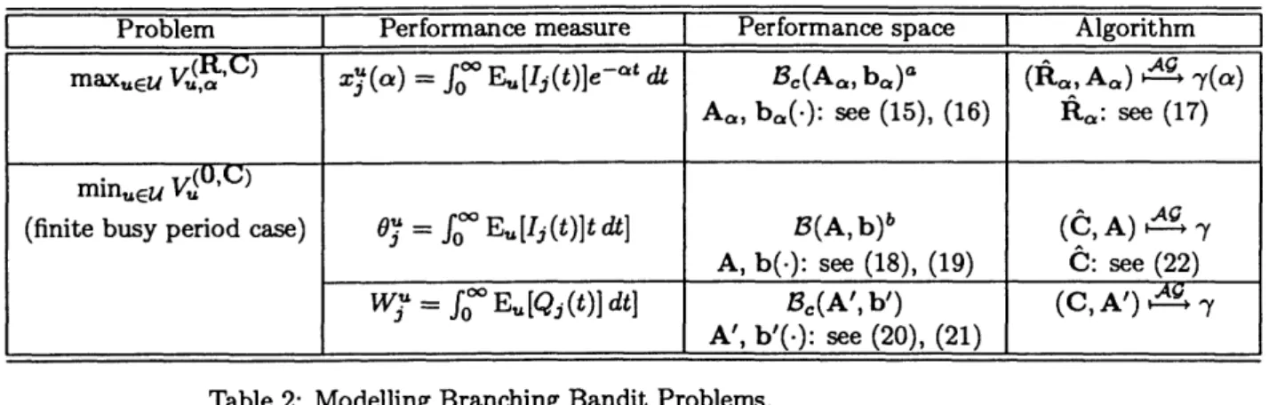
We shall refer to a project in state i as a type i job. In this section, we will define two different performance measures for a branching bandit process. The first one will be appropriate for modelling
a discounted reward-tax structure. The second will allow us to model an undiscounted tax structure. In each case we demonstrate what data is needed, what the performance space is and how the relevant parameters are computed.
Discounted Branching Bandits
Data: Joint distribution of vi, Nil,..., Ni , for each i:
',i(O) = i i(0, 1,..., 1),
mi, the number of type i bandits initially present, Ri, an instantaneous reward received upon completion
of a type i job, Ci, a holding tax incurred continuously while a type i job is in the system and a > 0, the discount factor.
Performance measure: Using the indicator
1 if a type j job is being engaged at time t; 0 otherwise,
the performance measure is
(a) Eu
[
-= e-atIj(t) dt. (14)Performance Space: The performance vector for branching bandits x"(a) satisfies conservation laws (a) EiEs AaZx'i(a) b(S), for S C E, with equality if policy u gives complete priority to Sc-jobs.
(b) ZiE Az x(a) = b(E).
Therefore, the performance space for branching bandits corresponding to the performance vector xu(a) is the extended contra-polymatroid base Bc(A,, b,). The matrix A, and set function bo(.) are calculated as follows:
A = 1 ,(a iES, SCE; (15)
Ti~1 Hqf)i(a ]
b.(S) = [ ()] SC
E
(16)jESc jEE
and the functions IS(0O) are calculated from the following fixed point system:
4iS(O)= b (O ) j=s. ls·), i E.
Objective function:
max V(R'C)(m) = kai,six(a) -Z miCi = Ri +Ci- E[Nj]Cj} ...(a) - m Ci
iEE iEE iEE jEE iEE
(17)
Undiscounted Branching Bandits
We consider the case that the busy period of the branching bandit process is finite with probability 1.
Data: E[vij, E[vi2], E[Nij]. Let E[N] denote the matrix of E[Nij). Performance measure:
1, if a type j job is being engaged at time t; 0, otherwise,
Qj(t) = the number of type j jobs in the system at time t.
0j = E
Ij (t)t dt]
j E
E.
W -
Eu [Qj(t)]
dt,
j
EE.
Stability: The branching bandits process is stable (its busy period has finite first two moments) if and only if E[N] < I (the eigenvalues of the matrix E[N] are smaller than one).
Performance space:
I. The performance vector Ou satisfies the following conservation laws:
(a) liEs ASOu < b(S), for S C E, with equality if policy u gives complete priority to Sc-jobs.
(b) EiEE AEO' = b(E).
The matrix A and set function b(-) are calculated as follows:
E[Ts]
As ETis] i E S, (18)
E[v,] ' and
(TS) ] + ~ E[vi] E[v] (E[T) E[(TS:)2]
b(S) = 2E[(T)2]-l E[(Tc)2]+ b(S ) E[ E[ 'i2] E[Yi]E1i2] EE[TSs ] E(TS )2]) /r (19)(19) where we obtain E[TS], Var[Tis] (and thus E[(Ts)2]) and E[vj] by solving the following linear systems:
E[Tis]= E[vi] + E E[Nij] E[TS], i E E;
jEs
Var[T J = Var[vi] + (E[Tj])TEs Cov[(Ni,)jes)] (E[T )js + E[Nij] Var[Tj], i E E; E[Ij] = mj + C E[NijlE[vi], j E. iEE Finally, E[Ts] = : mi E[Ti], iES VarlTm| = Z mi Var[TS]. iES
II. The performance vector WU satisfies the following conservation laws:
(a) iEs A'isW > b'(S), for S C E, with equality if policy u gives complete priority to S-jobs.
(b) ZieE A4EWiU = b'(E), where
A s = E[Ts], i E S, (20)
Problem Performance measure Performance space Algorithm maxEu V(,') xj'() fo= o E[Ij(t)]e- dt d Bc(Ac,, b,)a (A, ,A) 7 - (t )
A,, ba(-): see (15), (16) Ra: see (17)
min.u V( ' C )
minueU (
(finite busy period case) Oj = foo Eu[Ij(t)]t dt] B(A, b)b (C, A) ?t y A, b(-): see (18), (19) C: see (22) W = fo E[Qj(t)] dt] B3(A', b') (C, A') 4E -y
A', b'(-): see (20), (21)
Table 2: Modelling Branching Bandit Problems.
aExtended contra-polymatroid base bExtended polymatroid base
b'(S) = b(E) - b(S) + 2 E hiE[TS], (21)
iES
where row vector h = (hi)i E E is given by
h = m(I - E[N])-1Diag(( ( E [ ])E ar[v] )iEE)(I - E[N]),
and Diag(x) denotes a diagonal matrix with diagonal entries corresponding to vector x. Objective function:
min V.(O,C)
=
E,iO
+ 2
EChi
=
E (Ci-
E[Nij]Cj)
+2
ECihi
(22)
iEE iEE iE EEE E iEE
In Table 2 we summarize the problems we considered, the performance measures used, the conserva-tion laws, the corresponding performance space, as well as the input to algorithm Ag.
Given that branching bandits is a general problem formulation that encompasses a variety of prob-lems, it should not be surprising that the theory developed encompasses a large collection of problems. In Table 3 below we illustrate the stochastic control problem from the literature, the objective criterion, where the original indexability result was obtained and where the performance space was characterized. For explicit derivations of the parameters of the extended polymatroids involved the reader is referred to Bertsimas and Nifio-Mora [6].
2.4 Implications of the theory
In this section we summarize the implications of characterizing the performance space as an extended polymatroid as follows:
1. An independent algebraic proof of the indexability of the problem, which translates to a very efficient solution. In particular, Algorithm AS that computes the indices of indexable systems is as fast as the fastest known algorithm (Varaiya, Walrand and Buyukkoc [58]).
System Criterion Indexability Performance Space Batch of jobs LCa Smith [51]: Db Queyranne [43]: D, pc
Rothkopf [49] Bertsimas & Nifio-Mora [6]: P DCd Rothkopf [48]: D Bertsimas & Niiio-Mora [6]: P
Gittins & Jones [21]
Batch of jobs LC Horn [31]: D Bertsimas & Nifio-Mora [6]: EPe with out-tree Meilijson & Weiss [40]
prec. constraints DC Glazebrook [24] Bertsimas & Niiio-Mora [6]: EP Multiclass M/G/1 LC Cox & Smith [16] Coffman & Mitrani [15]: P
Gelenbe & Mitrani [20]: P DC Harrison [26, 27] Bertsimas & Nifio-Mora [6]: EP Multiclass M/G/c LC Federgruen & Groenevelt [18] Federgruen & Groenevelt [19]: P
Shanthikumar & Yao [50] Shanthikhumar & Yao [50]: P Multiclass G/M/c LC Federgruen & Groenevelt [18] Federgruen & Groenevelt [18]: P
Shanthikumar & Yao [50] Shanthikumar & Yao [50]: P Multiclass LC Ross & Yao [47] Ross & Yao [47]: P
Jackson network 9
Multiclass M/G/1 LC Klimov [35] Tsoucas [57]: EP
with feedback DC Tcha & Pliska [54] Bertsimas & Nifio-Mora [6]: EP multiarmed bandits DC Gittins & Jones [21] Bertsimas & Nifio-Mora [6]: EP Branching bandits LC Meilijson & Weiss [40] Bertsimas & Nifio-Mora [6]: EP DC Weiss [60] Bertsimas & Niiio-Mora [6]: EP Table 3: Indexable problems and their performance spaces.
aLinear cost
bDeterministic processing times CPolymatroid
dDiscounted linear reward-cost eExtended polymatroid
fSame service time distribution for all classes
gSame service time distribution and routing probabilities for all classes (can be node dependent)
2. An understanding of whether or not the indices decompose. For example, in the classical mul-tiarmed bandits problem Theorem 4 applies and therefore, the indices decompose, while in the general branching bandits formulation they do not.
3. A general and practical approach to sensitivity analysis of indexable systems, based on the well understood sensitivity analysis of linear programming (see Bertsimas and Nifio-Mora [6] and Glaze-brook [25]).
4. A new characterization of the indices of indexable systems as sums of dual variables correspond-ing to the extended polymatroid that characterizes the feasible space. This gives rise to new interpretations of the indices as prices or retirement options. For example, we can obtain a new interpretation of indices in the context of branching bandits as retirement options, thus general-izing the interpretation of Whittle [61] and Weber [59] for the indices of the classical multiarmed bandit problem.
5. The realization that the algorithm of Klimov for multiclass queues and the algorithm of Gittins for multiarmed bandits are examples of the same algorithm.
6. Closed form formulae for the performance of the optimal policy that can be used a) to prove structural properties of the problem (for example a result of Weber [59] that the objective function value of the classical multiarmed bandit problem is submodular) and b) to show that the indices for some stochastic control problems do not depend on some of the parameters of the problem. Most importantly, this approach provides a unified treatment of several classical problems in stochas-tic control and is able to address in a unified way their variations such as: discounted versus undiscounted cost criterion, rewards versus taxes, preemption versus nonpreemption, discrete versus continuous time, work conserving versus idling policies, linear versus nonlinear objective functions.
3
Restless bandits
In this section we address the restless bandit problem defined as follows: There is a collection of N projects. Project n E A = {1,..., N} can be in one of a finite number of states in E En, for n = 1, ... , N. At each instant of discrete time t = 0, 1, 2,..., exactly M < N projects must be operated. If project
n, in state in, is in operation, then an active reward RI is earned, and the project state changes into jn with an active transition probability pinj If the project remains idle, then a passive reward R is received, and the project state changes into jn with a passive transition probability pj. Rewards are discounted in time by a discount factor 0 < < 1. Projects are to be selected for operation according to an admissible scheduling policy u: the decision as to which M projects to operate at any time t must be based only on information on the current states of the projects. Let U denote the class of admissible scheduling policies. The goal is to find an admissible scheduling policy that maximizes the total expected discounted reward over an infinite horizon, i.e.,
Z* = maxEu O (t +.i + .. RiN(t) (23)
uEU t=o n(t
where in(t) and an(t) denote the state and the action (active or passive), respectively, corresponding to project n at time t. We assume that the initial state of project n is in with probability ain, independently of all other projects.
The restless bandit problem was introduced by Whittle [62], as an extension of the multiarmed bandit problem studied in the previous section. The latter corresponds to the special case that exactly one project must be operated at any time (i.e., M = 1), and passive projects are frozen: they do not change state (pi = 1, Pi 0 for all n E N and in #
jn).
Whittle mentions applications in the areas of clinical trials, aircraft surveillance and worker scheduling.In this section we review the work of Bertsimas' and Nifio-Mora [7], who build upon the work of Whittle [62] and propose a series of N linear relaxations (the last being exact) of the achievable region,
using the theory of discounted Markov decision processes (MDP) (see Heyman and Sobel [29]). They also propose an indexing heuristic that arises from the first of these relaxations.
In order to formulate the restless bandit problem as a linear program we introduce the indicators 1, if project n is in state in and active at time t;
I]n= 0, otherwise, and
P | 1, if project n is in state in and passive at time t; ,o-
{0,
otherwise.Given an admissible scheduling policy u E U we define performance measures
xi () = Eu[, I
(t)t
,
and x (u) = E[ IP(t)]3t]-t=O to
Notice that performance measure xi (u) (resp. x (u)) represents the total expected discounted time that project n is in state in and active (resp. passive) under scheduling policy u. Let
P= {X = (n (U))jEEaE{O1l}nEX I EU}
the corresponding performance space. As the restless bandit problem can be viewed as a discounted MDP (in the state space E1 x ... x EN), the performance space P is a polyhedron. The restless bandit problem can thus be formulated as the linear program
Z* =max E E R:anin.. (24)
P nEA iEE aE{O,1}
For the special case of the multiarmed bandit problem P has been fully characterized as an ex-tended contra-polymatroid. For the restless bandit problem we construct approximations of P that yield polynomial-size linear relaxations of the linear program (24).
3.1 A First-order Linear Programming Relaxation
The restless bandit problem induces a first-order MDP over each project n in a natural way: The state space of this MDP is En, its action space is A' = {0, 1}, and the reward received when action an is taken in state in is R~2. Rewards are discounted in time by discount factor P. The transition probability from
state in into state jn, given action an, is pn. The initial state is in with probability ain. Let
= {n = (Zix ())in EEn EA' I uEU}.
From a polyhedral point of view,
Q
is the projectiorr of the restless bandit polyhedron P over the space of the variables 2x for project n. From a probabilistic point of view,Q
is the performance space of the first-order MDP corresponding to project n. In order to see this, we observe that as policies u for the restless bandit problem range over all admissible policies U, they induce policies un for the first-orderMDP corresponding to project n that range over all admissible policies for that MDP. From the theory of discounted MDPs we obtain
Qn I jn + = a + n X E (25)
fxnr >J 0 I.- ,, J 5)nnZ E
inEEn an E{0,1}
Whittle [62] proposes a relaxation of the problem by relaxing the requirement that exactly M projects must be active at any time and imposing that the total expected discounted number of active projects over the infinite horizon must be M/(1 - 1). This condition on the discounted average number of active projects can be written as
z
i (u) =x EL[ zht=
[tB
1=-nEA iEEn t=O inEEn t=O
Therefore, the first-order relaxation can be formulated as the linear program
Z1 = max E E Ra"xa-n (26)
nEA iEn aE{O,1}
subject to o+. =+jX + En zXn,
in
EEn,
nE , Xi 7n Ji +nn inEEn anE{0,1} M ntEn iEEnWe will refer to the feasible space of linear program (26) as the first-order approximation of the restless bandit polyhedron, and will denote it as pl. Notice that linear program (26) has O(NIEm,,I) variables and constraints, where IEmax = maxnfI IEn I.
3.2
A kth-order Linear Programming Relaxation
We can strengthen the relaxation by introducing new decision variables corresponding to performance measures associated with kth-order project interactions. For each k-tuple of projects 1 < n <
... < nk < N, the admissible actions that can be taken at a corresponding k-tuple of states (il,..., ik) range over
Ak= { (al, .. ,ak) E {0,1}k a + + ak < M }
Given an admissible scheduling policy u for the restless bandit problem, we define kth-order perfor-mance measures, for each k-tuple 1 < n1 < < nk < N of projects, by
j ...Jk (U) = E[ IJl (t) * Ik (t) , j E En, , k E En (27)
The restless bandit problem induces a kth-order MDP over each k-tuple of projects nl < ·. < nk as follows: The state space of the MDP is E, x... x Enk, the action space is Ak, and the reward correspond-ing to state (in, ... ink) and action (a,, ... ank) is.Rn1 + .flI ' + J$) "k .Rewards are discounted in time
by discount factor fl. The transition probability from state (in,..., i,nk) into state (jn,.. .,
jk),
given action (an,, ank)I s *. .The initial state is (i,,. .. i,nk,) with probability ain inakAs in the first order relaxation all performance vectors in the k-th order relaxation satisfy
"l... -a = aj, +P Pj
Z
E...pl pk . j! E En ,...jk E Ek,(al,...,ak)EAk iiEnlikE
(al,...,ak)EAk
(28)
If u is an admissible scheduling policy, then
M
M
N-M 0 EZ
Z
ZC
i (U) (29) 1<nl<-..<nk<N i EE,,...,ikEE,, ( al +...+ak=r for max(0, k - (N - M)) < r < min(k, M). (30) Conservation law (29) follows since at each time the number of k-tuples of projects that contain exactlyr active projects is M N-M for r in the range given by (30). In terms of the orgina performance vectors
:I(U1)=
E a...ia(U).
(31)
(a1,...,ak)EAk
i EEn ,---ikEEk1
i,=i,a,=a
We now define the kth-order relaxation of the restless bandit problem as the linear program
Z
=
maxZ E E Rn znnE.J inEEn anE{0,1}
subject to (28), (29), (31) and nonnegativity constraints on the variables. We define the kth-order approximation to the restless bandit polyhedron P as the projection of the feasible space of the above linear program into the space of the first-order variables, xi, and denote it as pk. It is easy to see that
the sequence of approximations is monotone, in the sense that pl D p2 D ... D pN = p.
Notice that the kth-order relaxation has O(NkIEmaxk) variables and constraints, for k fixed. Therefore, the kth-order relaxation has polynomial size, for k fixed.
The last relaxation of the sequence is exact, i.e., ZN = Z*, since it corresponds to the linear
3.3
A Primal-dual Heuristic for the Restless Bandit Problem
The dual of the linear program (26) is
Z1 = min E E aj Aj, , + A (32)
nE. j E E
subject to
Ai -16 PinjnAjn >
Ri,
in EEn, n E , jn E EAi-P : PI injj + A2 > R, in En, n E A, j,n EE,
Let {: }, {A,,, A}, i E En, n E
K
be an optimal primal and dual solution to the first-order relaxation (26) and its dual. Let {7i" } be the corresponding optimal reduced cost coefficients, i.e.,-in = i
a-
ESpinjnj.
- RI.I
jnEEn
fftn =, Lin-p E ~, jn jn + X -. ,
jn EE,
which are nonnegative. It is well known (see Murty [41], pp. 64-65), that the optimal reduced costs have the following interpretation:
-ln is the rate of decrease in the objective-value of linear program (26) per unit increase in the value of the variable x.
~. is the rate of decrease in the objective-value of linear program (26) per unit increase in the value of
the variable x°,
The proposed heuristic takes as input the vector of current states of the projects, (il,..., iN), an optimal primal solution to (26), {jn }, and the corresponding optimal reduced costs, {7an }, and produces as output a vector with the actions to take on each project, (a*(il),..., a*(iN)). An informal description of the heuristic, with the motivation that inspired it, is as follows:
The heuristic is structured in a primal and a dual stage. In the primal stage, projects n whose corre-sponding active primal variable -X is strictly positive are considered as candidates for active selection. The intuition is that we give preference for active selection to projects with positive 1n with respect to those with in = 0, which seems natural given the interpretation of performance measure xi, (.) as the total expected discounted time spent selecting project n in state in as active. Let p represent the number of such projects. In the case that p = M, then all p candidate projects are set active and the heuristic stops. If p < M, then all p candidate projects are set active and the heuristic proceeds to the dual stage that selects the remaining M - p projects. If p > M none of them is set active at this stage and the heuristic proceeds to the dual stage that finalizes the selection.
In the dual stage, in the case that p < M, then M -p additional projects, each with current active primal variable zero (Yi, = 0), must be selected for active operation among the N - p projects, whose
actions have not yet been fixed. As a heuristic index of the undesirability of setting project n in state in, active, we take the active reduced cost -in. This choice is motivated by the interpretation of 1 stated above: the larger the active index 7ln is, the larger is the rate of decrease of the objective-value of (26)
per unit increase in the active variable xi". Therefore, in the heuristic we select for active operation the
M -p additional projects with smallest active reduced costs.
In the case that p > M, then M projects must be selected for active operation, among the p projects with 1 > 0. Recall that by complementary slackness, -1n = 0 if -ln > 0. As a heuristic index of the
desirability of setting project n in state in, active we take the passive reduced cost n. The motivation is given by the interpretation of -i°, stated above: the larger the passive index 0°
n is, the larger is the
rate of decrease in the objective-value of (26) per unit increase in the value of the passive variable x9°.°
Therefore, in the heuristic we select for active operation the M projects with largest passive reduced costs.
Assuming that the optimal solution of (26) is nondegenerate we can interpret the primal-dual heuristic as an index heuristic as follows:
1. Given the current states (il,..., iN) of the N projects, compute the indices
sin i Yin.
2. Set active the projects that have the M smallest indices. In case of ties, set active projects with Yi > 0.
In contrast with the Gittins indices for usual bandits, notice that the indices in for a particular project depend on characteristics of all other projects. Bertsimas and Nifio-Mora [7] report computational results that show that the primal-heuristic and the bound given by the second order relaxation are very close, proving that both the relaxation and the heuristic are very effective.
4 Polling systems
Polling systems, in which a single server in a multiclass queueing system serves several classes of cus-tomers incurring changeover times when he serves different classes, have important applications in com-puter, communication, production and transportation networks. In these application areas several users compete for access to a common resource (a central computer in a time sharing computer system, a transmission channel in a communication system, a machine in a manufacturing context or a vehicle in transportation applications). As a result, the problem has attracted the attention of researchers across very different disciplines. The name polling systems comes primarily from the communication literature. Motivated by its important applications, polling systems have a rather large literature, which for the most part addresses the performance of specific policies rather than the optimal design of the polling
system. For an extensive discussion of the research work on polling systems, we refer to the survey papers by Levy and Sidi [37] and Takagi [52], [53].
Consider a system consisting of N infinite capacity stations (queues), and a single server which serves them one at a time. The arrival process to station i (i = 1, 2,..., N) is assumed to be a Poisson process with rate Ai. The overall arrival rate to the system is A = N1 Ai. Customers arriving to station
i will be referred to as class-i customers and have a random service requirement Xi with finite mean
xi and second moment 2) The actual service requirement of a specific customer is assumed to be
independent of other system variables. The cost of waiting for class-i customers is ci per unit time. There are changeover time dij whenever the server changes from serving class-i customers to class-j customers. The offered traffic load at station i is equal to pi = Aixi, and the total traffic load is equal to p =i l Pi
The natural performance measure in polling systems is the mean delay time between the request for service from a customer and the delivery of the service by the server to that customer. The optimization problem in polling systems is to decide which customer should be in service at any given time in order to minimize the weighted expected delay of all the classes. Let U be the class of nonpreemptive, non-anticipative and stable policies. Within U we further distinguish between static (Ustatic) and dynamic (Udynamic) policies. At each decision epoch static policies do not take into account information about the state of stations in the system other than the one occupied by the server and are determined a priori or randomly. In particular the server's behavior when in station i is independent of the state of the other stations in the system (i.e., the queue lengths and the interarrival times of the customers). Examples of static policies include randomized policies, in which the next station to be visited by the server is determined by an a priori probability distribution, and routing table policies, in which the next station to be visited is predetermined by a routing table. A special case of the routing table policies is the cyclic policy, where the stations are visited by the server in a cyclic order.
Dynamic policies take into account information about the current state of the network. For example, a threshold policy or a policy that visits the most loaded station, is a dynamic policy, because the decision on which customer to serve next by the server depends on the current queue lengths at various stations in the system. In certain applications it might be impractical or even impossible to use a dynamic policy. For example in a transportation network, the vehicle might not know the overall state of the network. As a result, although static policies are not optimal, they can often be the only realistic policy. Moreover, when there are no changeover times, the policy that minimizes the mean weighted delay is an indexing policy (the c rule), a static policy.
While the literature on performance analysis of polling systems is huge there are very few papers addressing optimization. Hofri and Ross [30] and Reiman and Wein [46] address the optimization problem over dynamic policies for polling systems with two stations. Boxma et. al. [13] propose heuristic polling table strategies. In this section we review the work in Bertsimas and Xu [10] in which a nonlinear (but
convex) optimization problem is proposed, whose solution provides a lower bound on an arbitrary static policy. Using information from the lower bounds and integer programming techniques, static policies (routing table policies) are constructed that are very close (within 0-3%) to the lower bound.
4.1
Lower bounds on achievable performance
We develop in this section lower bounds on the weighted mean waiting time for polling systems for nonpreemptive, nonanticipative and stable policies. We call these policies admissible. We present bounds for both static and dynamic policies.
Let E[Wi] be the average waiting time of class-i customers. The goal is to find a static policy
u E Usttic to minimize the weighted mean delay E[W] for the polling system:
N
Umin E[W]= ZcAiE[Wi]. (33)
i=1
Within a particular class, we assume that the server uses a First-In-First-Out (FIFO) discipline. We denote with dij the changeover time when the server changes from serving class-i customers to class-j customers (i, j = 1, 2,..., N).
Theorem 5 The optimal weighted mean delay in a polling system under any static and admissible policy is bounded from below by Zstatic, the solution of the following convex programming problem:
Z.tatic = min 2 Ei=l I, + E c,,(1-p) (34)
i1
-p
(Ej=, mj )
subject to N= mij -kl mki = , i= 1,2,...,N (35)
Ei,=> dijmi 1 - p (36)
mii = 0, mij 0 V i, j,
The mij in the above convex optimization problem represent the steady state average number of visits from station i to station j per unit time. Constraint (35) represents conservation of flow, while (36) is the stability condition. These constraints are still valid even under dynamic policies. The fact that the objective function in (34) represents a lower bound for the optimal solution value, only holds for static policies. The idea of the proof is that under a static policy, the expected waiting time of class i customers decomposes to
A(Z( ) v(2) 2(1 - pi) 2vi
where vi, vi(2) are the first and second moments of the vacation times observed at station i. Using the inequality v(2) > v2 and expressing the expected vacation times vi in terms of mij we obtain the bound. For details see Bertsimas and Xu [10]. Notice that while the feasible space of (34) is a network flow problem with a side constraint, the objective function is a nonlinear, but convex function.
In order to acquire further insight on the bound of the previous theorem, the flow conservation constraints (35) are relaxed to obtain a closed form formula for the lower bounds.
Theorem 6 a) The weighted mean delay in a polling system under any static and admissible policy is bounded from below by:
Zclo=d 1 di (37)
Zcloaed
~
ciAi 2 ) + ( l c(1 - pi)d*)2 (3)2i\ 1 -Pi 2A(1 - p)
where d! = dj(i),i = minj{dji}.
b) For a homogeneous polling system (ci = 1, xi = x, for all i = 1, 2,..., N), under static and admissible
policies, the weighted mean delay is bounded from below by:
,x
(1 p,)d;)2-
(
(38)
2(1 - ) + 2A(1 - p)
Notice that the bound from (38) is stronger than (37) for the special case of a homogeneous system. For arbitrary policies including dynamic ones we can prove the following.
Theorem 7 The optimal weighted mean delay in a polling system under any admissible policy is bounded
from below by
Zdynamic = max{ [N 2j [E 1 (1-iAi
1
~
:~'Z) -X2
) l--p minjEN{ il xjij + 'i 'E=
where ai = pj=1 Pj and p = 1 pj is the system utilization.
The first term in the lower bound represents the optimal weighted mean delay with no changeover costs (the optimal policy corresponds to the cp rule), while the second term incorporates changeover times in the lower bound.
4.2
Design of effective static policies
The goal of this subsection is to provide a technique to construct near optimal policies using integer programming. As already mentioned the mij are interpreted as the steady state average number of visits from station i to station j per unit time. Let eij = mij/ -k,l mk and E = [eij] be the corresponding changeover ratio matrix. Intuitively, in order for the performance of a policy u to be close to the lower bound, it is desirable that the proportion of changeovers from station i to station j under the policy u is close to eij. We refer to this requirement as the closeness condition. We consider two classes of policies that satisfy the closeness condition approximately.
Randomized policies:
Under this class of policies the server after serving exhaustively all customers at station i moves to station j with probability Pij. Kleinrock and Levy [34] consider randomized policies, in which the next station visited will be station j with probability pj, independent of the present station.