Aerodynamic fuze characteristics for trajectory control

Aerodynamic Fuze Characteristics

for Trajectory Control

by

Alexander Michael Budge

B.S., Aeronautical Science and Engineering

and Mechanical Engineering

University of California, Davis (1996)

Submitted to the Department of Aeronautics and Astronautics

in partial fulfillment of the requirements for the degree of

Master of Science in Aeronautics and Astronautics

at the

MASSACHUSETTS INSTITUTE OF TECHNOLOGY

June 1998

@

Massachusetts Institute of Technology 1998. All rights reserved.

Author ... ...

Department of Aeronautics and Astronautics

May 20, 1998

Certified by...

Eric Feron

Assistant Professor

Thesis Supervisor

A ccepted by ...

Jaime Peraire

S-" -

_{Chairman, Department Graduate Committee}

. , .iOLOGY

Aerodynamic Fuze Characteristics

for Trajectory Control

by

Alexander Michael Budge

Submitted to the Department of Aeronautics and Astronautics on May 20, 1998, in partial fulfillment of the

requirements for the degree of

Master of Science in Aeronautics and Astronautics

Abstract

Recent development of micromechanical Inertial Management Units (IMUs) and Global Positioning Systems (GPS) capable of withstanding more than 16,000 g's has spawned renewed interest in unpowered guided munitions. Guidance schemes seek to increase the static targeting accuracy by decreasing the Circular Error Probability (CEP). In order to retain the usefulness of the vast stock piles of Army/Navy/USMC am-munition, numbering in the tens of millions of rounds, a fuze replacement is sought which incorporates all the necessary additions to transform these unguided shells into guided, or competent munitions. In particular, competent munitions require aerody-namic control actuation to effect trajectory control. Investigations focus on replace-ment fuzes for trajectory control by modulated roll control of a fixed magnitude lift

vector.

Trajectory simulations with a modified point mass model reveal that typical bal-listic trajectories exhibit an approximately invariant Mach number distribution for a range of launch angles. The trim lift coefficient is introduced as a figure of merit and simulations show the crossrange deflection of a trajectory to be very sensitive to the transonic distribution of the trim lift coefficient.

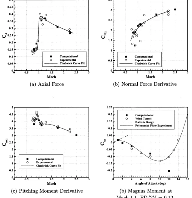
The development of grid generation processes and the implementation of Navier-Stokes CFD methods provide a means to investigate the underlying aerodynamic behavior of lift and torque generating geometric asymmetries. To engender confi-dence, the flow simulation is validated against wind tunnel and ballistic range data for baseline geometries.

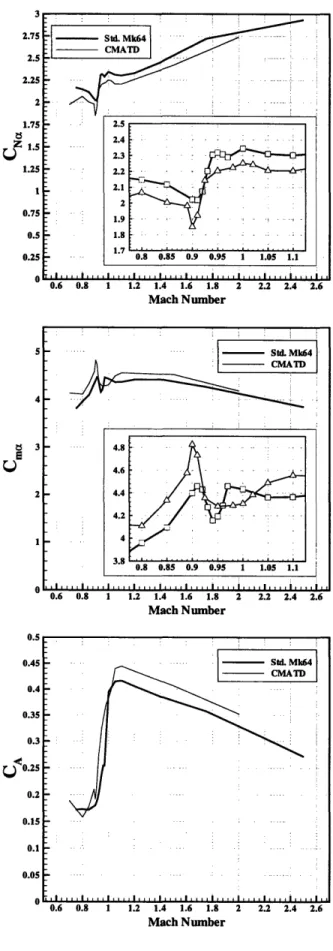
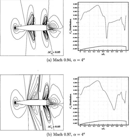
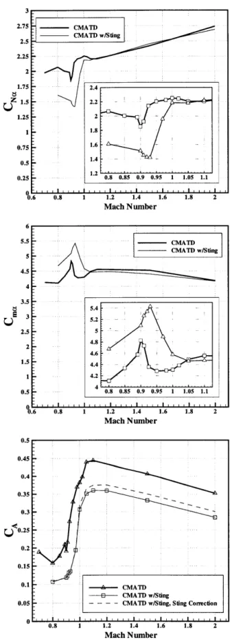
Baseline computations identify four modes of transonic critical behavior related to the Mach dependent location of shocks on boat-tailed projectiles. Calculations with a spinning boundary condition capture the small angle of attack sign change of the Magnus moment, revealing that the sign change results from the contribution of the last 2% of the body length. Baseline computations also show that sting mounted wind tunnel models affect the pressure recovery over the boattail region at transonic Mach numbers, producing large errors in the wind tunnel modeling of transonic critical

Sliced and bent configurational asymmetries are examined as candidate lift gen-erating geometries, but are found to be inefficient in that the asymmetries do not actuate the flow as intended with the net trim lift resulting primarily from residual aerodynamic effects and not from the high pressure surface of the asymmetry.

A leveraged boundary layer actuation concept is then pursued as a more efficient lift generating mechanism. Relatively small scale deviations in boundary layer de-velopment can drive transonic critical behavior producing large resultant trim forces, which can work synergistically with the transonic trajectory sensitivity to produce large maneuvering envelopes.

Finally, the thesis examines aerodynamic torque generation with short body-fitted and differentially canted strakes. An empirical design algebra for dual strakes can be written to simplify preliminary design, but computations show that the strakes interact such that performance does not scale directly with the number of strakes. Thesis Supervisor: Eric Feron

Title: Assistant Professor

Thesis Supervisor: Eugene Covert Title: Professor Emeritus

Acknowledgments

A brief acknowledgment of the usual suspects is in order. First, I would like to thank the people who have supported and encouraged me throughout my life; the people who seldom put their interests before mine; who have never been my adversaries, never sought to tear me down, but when my ratiocination became confused or when I have lost perspective on life they have restored me with kindness and humility. Primary among these are my mom and dad who made the effort to be my parents and my friends, but also the enumerable others who have given of themselves to be my friends. In a world in which it seems everyone wants to be the best, true friends are more than priceless, they give life.

I would like to thank Professor Eric Feron, my thesis supervisor and academic advisor, for the encouragement and support he has provided during my first two years of graduate education at MIT. I would also like to thank Professor Eugene Covert, my other thesis supervisor, for challenging me to think clearly and critically as well as for sharing the two directives of technical presentation: "Don't suppress the zero!" and "Your goal is not to make it possible to understand, but to make it impossible not to understand."

I would like to thank Bob Haimes for providing the computational resources that made the project happen.

Sean George, my research cohort, deserves thanks not only for being there for external processing over an inky black cup of Tosci's french roast, but also for being my friend.

I am also indebted to Earl P.N. Duque of the US Army Aeroflightdynamics Di-rectorate at the NASA Ames Research Center for his help in getting setup with

Contents

1 Introduction

1.1 Concept of Competent Munitions 1.2 Projectile Dynamics ...

1.2.1 Dynamic Motion ... 1.2.2 Linearized Trim State .. 1.2.3 Ballistic Trajectory .... 1.3 Figure of Merit ...

1.4 Contributions ... 1.5 Overview ... 2 Aerodynamic Modeling

2.1 Requirements and Model Selection . . . . 2.2 Grid Generation ...

2.2.1 Surface Domain Decomposition and 2.2.2 Surface Grid Generation ... 2.2.3 Volume Grid Generation . . . . 2.2.4 Overlapped Connectivity . . . . 2.3 Numerical Convergence . . . . 2.3.1 Spatial Convergence . . . . 2.3.2 Temporal Convergence . . . . 2.4 Boundary Conditions . . . . 2.5 Validation ... 2.5.1 SOCBT Configuration . . . . Grid Topology . . . .• . 17 . . . . 17 . . . . 20 . . . . 22 . . . . 23 . . . . 24 . . . . 26 . . . . 30 . . . . 3 1 33 33 ... . 35 . . . . . . 36 ... . 37 . . . . . . 41 . . . . . . 42 . . . . . . 43 . . . . . . 43 . . . . . . 45 . . . . . . 47

2.5.2 Mk41 5"/54 Configuration ... .

3 Baseline Aerodynamic Behavior 3.1 Baseline Profiles ...

3.2 Mach Behavior ...

3.3 Transonic Critical Behavior . . 3.4 Sting Effects ...

3.5 Magnus Characteristics ...

4 Configurational Asymmetries for Lift Generation 4.1 Concept and Description of Geometries . . . . 4.2 Angle of Attack and Sideslip Angle Behavior . . . 4.3 Parametric Study ...

4.4 Aerodynamic Behavior ...

4.4.1 Aerodynamics of the Bent Fuze . . . . 4.4.2 Aerodynamics of the Sliced Fuze . . . . . 4.4.3 Aerodynamics of Normal Force Generation 4.5 Mach Behavior ...

4.6 Magnus Characteristics . . . . 4.7 Design Considerations . . . . 5 Leveraging Sensitivities for Lift Generation

5.1 Concept and Description of Geometry . . . . 5.2 Angle of Attack Behavior . . . . 5.3 Mach Behavior ...

5.4 Design Considerations . . . . 6 Canted Strakes for Torque Generation

6.1 Concept and Description of Geometry . . . . 6.2 Angle of Attack and Sideslip Angle Behavior . . . 6.3 Parametric Study ... 6.4 Design Considerations . . . . 67 . . . . . 67 . . . . . 68 .... . 70 . . . . . 73 . . . . . 73 . . . . . 78 . . . . . 82 . . . . . 85 . . . . . 89 . . . . . 91 95 95 97 99 102 105 . . . . . 106 . . . . . 107 ... 108 . . . . . 110 53 . . . . 53 . . . . 55 . . . . . 55 . . . . 60 . . . . . 63

7 Conclusions and Future Work 113

A Trim State Linearization 117

B OVERFLOW Flow Solver Code Suite 121

B.1 OVERFLOW Flow Solver ... 121

B.2 HYPGEN Volume Grid Generator ... 124

B.3 PEGSUS Connectivity Solver ... 125

B.4 CHIMERA Grid Tools ... 125

List of Figures

1-1 Depiction of Spiraling Fixed-Trim Trajectory . ... 20

1-2 Aeroballistic Coordinate System ... .. 21

1-3 Gyroscopic Behavior of Spin-Stabilized Projectile . ... 23

1-4 Behavior of a Typical Ballistic Trajectory . ... 25

1-5 Maneuvering Envelope Behavior ... .. 27

1-6 Range Variation with CLtrim ... 28

1-7 Crossrange Sensitivity to Mach Local CLtrim Perturbations ... 28

2-1 Axisymmetric Surface Grid and Computational Coordinate System 38 2-2 Component and Resultant Grids for Sliced Geometry . ... 39

2-3 Strake Grid Topology and Geometry . ... 41

2-4 Half-Plane Showing Structured Volume Grid . ... 42

2-5 Spatial Convergence in Two Orthogonal Surface Directions ... 44

2-6 Steady-State and Time Accurate Temporal Convergence ... 46

2-7 Basic SOCBT Configuration ... 48

2-8 Pressure Distribution Comparisons for SOCBT Configuration . . .. 49

2-9 Qualitative Flow field Comparison . ... . 50

2-10 Comparison of Mach Behavior for Mk41 Projectile . ... 51

3-1 Baseline Profiles . . . 54

3-2 Mach Behavior of Baseline Configurations . ... 56

3-3 Transonic Critical Behavior Part I . ... . 57

3-4 Transonic Critical Behavior Part II . ... 59

3-6 Boattail Flow Field Comparison for Free Flying and Sting Geometries 62

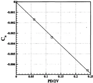
3-7 Linearity of Magnus Moment with Spin Rate . ... 63

3-8 Distribution and Development of Magnus Force and Moment .... . 64

4-1 Parametric Definitions for Configurational Asymmetries ... . 68

4-2 Pitch and Yaw Linearity at Mach 1.1 . ... . . . 69

4-3 Aerodynamic Behavior with Configurational Parameter Variations . 71 4-4 Trim State Behavior with Configurational Parameter Variations . . . 72

4-5 Bent Configuration Pressure Distributions . ... 74

4-6 Bent Configuration Boundary Layer Behavior at Mach 1.1 ... 76

4-7 Transonic Critical Behavior of Bent Configuration . ... 77

4-8 Bent Configuration Boundary Layer Behavior at Mach 0.90 ... 78

4-9 Sliced Fuze Pressure Distributions at Mach 1.4 . ... 79

4-10 Sliced Configuration Pressure Distributions at Mach 1.1 ... . 80

4-11 Boundary Layer Behavior for Two Slice Angles at Mach 1.1 .... . 81

4-12 Normal Force and Pitch Moment Development at Mach 1.1 ... 81

4-13 Comparison of Slender Body Theory and Computation ... 84

4-14 Force and Moment Development Comparison of Sliced and Bent Con-figurations at M ach 1.1 ... 86

4-15 Aerodynamic Variation with Mach number for Configurational Asym-metries ... 87

4-16 Trim State Variation with Mach number for Configurational Asymmetries 88 4-17 Effects of Parameter Variations on Magnus for Bend at 4.25" and 500 Slice . . . .. .. . 89

4-18 Magnus Development over Configurational Asymmetries ... . 90

4-19 Maneuvering Envelopes of Representative Configurational Asymmetries 92 5-1 BLAM Fuze Concept ... 96

5-2 The BLAM Fuze at Mach 0.95 and Zero Angle of Attack ... . 97

5-3 Normal Force and Pitch Moment Behavior with Angle of Attack . . . 98

5-5 Trim Lift Variation with Mach Number . ... 101

5-6 Maneuvering Envelope ... 102

6-1 Description of Strake Geometry ... .. 106

6-2 Roll Torque Variation with Angle of Attack and Sideslip Angle .... 107

6-3 Static Roll Torque Generation ... 109

6-4 Pressure Distribution Over Strake: Geometry 3 at 200, Mach 2.0, and Zero Angle of Attack ... 111

A-1 Coordinate System for Rotational Motion Analysis . ... 117

A-2 Rotational Motion ... 119

C-1 Grid Spacing Source Element ... ... 129

List of Tables

2.1 Hierarchy of Configurational Flow Modeling . ... 34 6.1 Defining Parameters of Strake Geometries . ... 108 6.2 Dual Strake Torque Scaling Parameters . ... 110

Chapter 1

Introduction

The computational investigation of aerodynamic control actuator design of replace-ment fuzes for guided projectiles has four constitutive components: competent mu-nitions, projectile dynamics, computational modeling, and projectile aerodynamic behavior. The components are combined to seek an effective pressure distribution for trajectory control. The competent munitions concept, as described in the next section, establishes the engineering framework for the design problem, while an understanding of projectile dynamics is important to the interpretation of design fitness. Computa-tional modeling addresses the analysis engine utilized to investigated the problem, in particular, how CFD simulation can be applied to the design of a complicated aerody-namic system in a reliable manner. Computations elucidate characteristic projectile aerodynamic behavior. Finally, all four of the components are assembled to develop aerodynamic characteristics of replacement fuzes for guided projectiles.

1.1

Concept of Competent Munitions

Guidance of gun-launched munitions has been visited and revisited for decades, but reliable and cost-effective guided munitions have yet to be developed. Recent ad-vances in technology and a fertile marketplace have renewed interest in unpowered guided munitions. Micro mechanical Inertial Management Units (IMUs) and Global Positioning Systems (GPS) capable of withstanding more than 16,000 g's have been

developed recently which could potentially be embedded in the fuze of a standard artillery round, allowing such a round to be converted into a highly accurate guided munition. The fuze of a projectile is the front end component which is used to arm and trigger the munition. Such conversions retain the usefulness of the vast stock piles of Army/Navy/USMC ammunition which number in the tens of millions of rounds. Guidance schemes seek to increase the static targeting accuracy by decreasing the Circular Error Probability (CEP). The goal is to reduce the CEP for 30-kilometer shot two orders of magnitude, from the current CEP of about 250 meters to only a few meters. Although the modified rounds will be more expensive than standard unguided rounds, they will be cost-effective because fewer rounds will be needed per target and the logistical burden of storing, transport and handling will be lower for the mission. The resulting increase in the rate of successful hits and reduction in the rate of unwanted hits has given this concept the name competent munitions.

Several different approaches to competent munitions are currently being explored: auto-registration, range only correction, as well as combined range and crossrange correction. In the auto-registration concept, a test round capable of communicating its impact point back to the gun is launched periodically so that appropriate cor-rections can be made to the gun inclination and direction. This helps to account for consistent atmospheric unknowns, such as wind and temperature. Range only correction requires single axis control authority. The simplest idea utilizes a drag increasing spoiler, which can be actuated by the controller to correct the range after intentionally overshooting the round. Range and deflection concepts require two axis control authority, such as a movable canard actuation system.

The tendency of low drag projectile shapes to be aerodynamically unstable neces-sitates some method of stabilization. The two most common methods are gyroscopic stabilization by spinning and aerodynamic stabilization by mounting fins behind the center of gravity. Projectiles can also be flare-stabilized by using a profile with increas-ing cross-sectional area behind the center of gravity, but this incurs a drag penalty and is uncommon. Most spin-stabilized projectiles use a profile with a section of decreasing cross-sectional area leading to the base, called a boattail. A boattail will

decrease drag, but increase the static instability of a projectile. Two axis controllers typically require that the fuze of a spin-stabilized projectile be "despun" to provide azimuthal or roll authority for the actuator. Despinning can be partial or complete. Complete despinning seeks to give total authority over the azimuthal orientation in inertial space, while partial despinning significantly reduces the spin rate of the fuze relative to body of the projectile, but does not give authority over the azimuthal orientation. GPS signal acquisition and IMU stabilization requirements also place constraints on the fuze spin rate.

In addition to difficulties of developing miniature avionics capable of handling the high-g operating environment, there has been difficulty in designing mechanically re-liable and cost effective aerodynamic control actuation schemes. In order to minimize impact to the handling and loading procedures and equipment, all of the electronics and mechanical actuators must fit inside a standard fuze, which has an 8.5 cubic inch external volume. Previous attempts have been based on movable canards, such as in the CHAMP [17] concept, which require expensive mechanical systems containing many moving parts. To date, such systems have proven to be unreliable and have required almost the full fuze volume for the actuation mechanism.

Non-canard based actuation, the subject of this thesis, has been explored before previously for small caliber (30mm) aircraft fired projectiles. McGinley [19] found that articulating the nose of a spin-stabilized projectile provides sufficient lateral ac-celeration for both air-to-air and air-to-surface guidance with small deflection angles. Unfortunately, the aerodynamic coefficients were estimated by treating the nose and aft sections of the projectile as independent, a grossly incorrect assumption as will be shown in Chapter 4.

Past concepts for two axis control have required both direct azimuthal and lift magnitude control. Most frequently, variable deflection canards are mounted on com-pletely despun fuzes, as in the CHAMP concept. Draper Laboratory has envisioned a fixed-trim terminal guidance concept which gives two axes of control authority by modulating the azimuthal orientation of a fixed normal force, as developed by Gracey, et. al. [12] for maneuvering re-entry of strategic missiles. By fixed lifting force, it

is not intended to imply a constant normal force over the trajectory, but that the controller has no authority over the magnitude of the force. Such control schemes result in a spiraling trajectory, as Figure 1-1 depicts. Trajectory simulations have shown that a fixed-trim guidance concept is a viable and promising guidance scheme for competent munitions.

Figure 1-1: Depiction of Spiraling Fixed-Trim Trajectory

Once the requirement for generating a lifting force of controllable magnitude has been removed, it becomes possible to design asymmetries into the fuze shape which generate the necessary, but fixed, normal force. These asymmetries are the focus of this thesis. The next two sections will introduce the dynamic behavior of spin-stabilized projectiles and a figure of merit for evaluating design fitness.

1.2

Projectile Dynamics

An understanding of the rigid body dynamics of projectile motion is important to both the general goals of the aerodynamic design process and to the particular details of applying the results. Figure 1-2 establishes the aeroballistic coordinate system for describing forces and moments.

The reference geometric dimensions are defined as:

L length of projectile

D maximum diameter of projectile

S area corresponding to maximum diameter

CAA Dj

CZ, Fz

Mz

Figure 1-2: Aeroballistic Coordinate System

conditions have the nomenclature: .freestream speed of sound

freestream Mach number

freestream Temperature (absolute)

freestream Reynolds number, aoopooL/Poo dynamic pressure, pPooaooM

freestream velocity spin rate pitch rate The aerodynamic CA CN CN, Cm Cm. C,m + Cm,

coefficients have the following definitions: axial force coefficient

N

normal force coefficient,

_QS

normal force coefficient derivative, 9 pitch moment coefficient, QSD

QCm

pitch moment coefficient derivative, 9a

pitch damping moment coefficient sum, pitch damping moment coefficient sum, _{09 D} -a

VOO The flight aoo M, Too Re

Q

C, yaw or Magnus moment coefficient, QSD

Cn,, Magnus moment coefficient derivative, na C, roll moment coefficient, QSD

CI, roll damping moment coefficient,

Y

Cy side or Magnus force, QS

Cy,, _{Magnus force coefficient derivative,}

1.2.1

Dynamic Motion

After leaving the gun barrel, the projectile enters into a complex oscillatory motion about its center of mass. Conservation of angular momentum states that the spin (angular momentum) vector always tends to rotate toward the moment vector. An initial disturbance in pitch angle of attack will generate a pitch moment, but this pitch moment will result in rotational motion in the yaw plane due to the angular momentum of the spinning mass, as illustrated in Figure 1-3. The resulting yaw angle will cause the moment vector to dip below the yaw plane and the process repeats, producing counterclockwise rotation of the moment vector- classic gyroscopic motion. The spin vector will rotate about the original axis from which it was displaced because the gyroscopic couple was zero when the body was aligned with that axis. Thus the projectile will precess about the relative wind. In addition to this relatively low frequency precessional mode, there also exists a higher frequency nutational mode resulting from the total angular velocity not being parallel to a principle axis of inertia.

The tendency to precess about the axis of the relative wind causes the projectile to remain aligned with the trajectory, provided that the precession rate is high enough1_.

This alignment tendency biases the precession such that there is a net yaw angle, called the yaw of repose. The yaw of repose is perpendicular to the plane defined by the direction of the change in flight path angle and the relative wind. Projectiles

1This requirement establishes the upper bound on the spin rate for stabilization. The precession rate should be much higher than the rate of change of the flight path angle

Figure 1-3: Gyroscopic Behavior of Spin-Stabilized Projectile

typically spin clockwise as viewed from the rear resulting in a negative yaw of repose, causing the trajectory to drift to the left.

1.2.2

Linearized Trim State

Properly stabilized projectiles precess at a rate which is high enough to allow the motion to be linearized about the precessional axis by time averaging the motion.

Asymmetric aerodynamic forcing from the change in flight path angle and control forces bias the mean total pitch angle of the projectile. The projectile will oscillate about the instantaneous axis of zero moment, which is the trim axis for the linearized system. The yaw of repose results from the time averaged spin vector precessing in the vertical plane. The instantaneous yaw of repose can be calculated assuming steady precession:

_ IzzM (1.1)

repose = QSDCm(

where y is the rate of change of the flight patch angle.

The fixed trim aerodynamic actuation under consideration can be modeled as a zero-offset moment coefficient Cmo and a normal force coefficient CNo. The normal force vector generated by the geometric asymmetry and the axis of revolution define the asymmetry plane. For mirror symmetric asymmetries, this is simply the lateral symmetry plane. The zero-offset moment results in a linearized trim angle of attack in the asymmetry plane, as verified in Appendix A.

Otrim = -mo (1.2)

1.2.3

Ballistic Trajectory

The ballistic trajectory of the projectile determines the mission profile of the vehicle. The nature of the trajectory is important for the design of aerodynamic actuation, as it determines the fundamental aerodynamic similarity parameters Mach number and Reynolds number. While aircraft are often designed for a single design point, con-sisting of a single Mach number and Reynolds number, projectiles must be designed for a specified time distribution of Mach numbers and Reynolds numbers.

The trajectory resulting from an initial velocity of 2650.0 ft/s, a quadrant elevation (launch inclination) of 25.0 degrees and a spin rate of 255 Hz has been used as a nominal trajectory. Figure 1-4 gives some outputs of interest calculated with a modified point mass model.

The effect of quadrant elevation on the behavior of the ballistic trajectory has an important consequences for trajectory control. The three quadrant elevations com-puted have widely varying altitude profiles and a four mile downrange variation, yet they produce trajectories with nearly identical Mach number and crossrange distri-butions. The invariant Mach distribution is a rather fortuitous circumstance because it makes the aerodynamic performance of the control actuator inherently robust to variations in the quadrant elevation due to the relative insensitivity of aerodynamic performance to Reynolds number for projectiles of this type. The dynamic pressure distribution, while varying moderately over the three quadrant elevations, maintains form, indicating that the optimal design solution for one trajectory will most likely not be too far from the optimal for other trajectories, with performance degradation being an unavoidable result of shorter flight time.

24000 22000 20000 18000 16000 14000 12000 10000 8000 6000 4000 2000 0 5 10 15 20 25 30 35 40 45 50 55 60 65 Time (sec)

(a) Altitude and Crossrange

QE = 15.0 and VO = 2650 ft/s QE = 25.0 and V0 = 2650 ft/s - - QE = 35.0 and V0 = 2650 ft/s I . .. . . 0 , - .. . . . "0 5 1750 1250S 1000 750 U 10 15 20 25 30 35 40 45 50 55 60 65 Time (sec) (c) Reynolds Number 0 5 10 15 20 25 30 35 40 45 50 55 60 6 Time (sec) (b) Mach Number Time (sec) (d) Dynamic Pressure Figure 1-4: Behavior of a Typical Ballistic Trajectory

--- QE = 15.0" and VO = 2650 ft/s - QE = 25.0- and VO = 2650 ft/s - - - QE = 35.0 and VO = 2650 fts QE = 15.0' and VO = 2650 ft/s - QE = 25.0' and VO = 2650 ft/s - - - - QE = 35.0' and V0 = 2650 ft/s 71Hil _{i - i i} LL I) ( -1, ,, .. I I I ~~ ..~~ ~ I I I .. I ~ ~ I .. .. 1 flI,

1.3

Figure of Merit

The purpose of the figure of merit is two-fold. First, it should provide a simple means of evaluating the fitness of a given configuration by bypassing the need to run nu-merous trajectory simulations. This purpose leads us to formulate the figure of merit in terms of aerodynamic coefficients, which allows us to move directly from aero-dynamic characteristics to an indication of relative aero-dynamic performance. Second, together with the parameterization of the configuration, the figure of merit should facilitate the collapse of data. The figure of merit encapsulates the dynamic behavior of the design and casts it in the language of aerodynamics.

The broad range of Mach numbers experienced by the projectile over its trajec-tory and the varying relationship between the distribution of Mach numbers and the launch conditions governing the trajectory make it difficult to define a concise and unambiguous figure of merit, as we can often do for single point designs. A comprise is made between accuracy and utility by choosing a point figure of merit which does not assume a Mach distribution, but augmenting the figure of merit with information

about Mach sensitivity.

The figure of merit chosen is the trim lift coefficient, CLtrim, which is derived from the linearized trim state. The yaw of repose is not included in the "trim" coefficient, it represents the linearly independent reaction to the control moment. The trim lift coefficient is chosen because it is the force perpendicular to the trajectory, to which the relative wind is tangent. The yaw angle due to control is given by Equation 1.2, with which the trim lift coefficient can be written:

CLtrim = (CNo + CN,. trim) cos atrim - CA sin Otrim (1.3) The trim lift quantifies accurately the effectiveness of a given design at a single Mach number, but it does not quantify the resultant crossrange performance. Cross-range performance prediction requires knowledge of how the design behaves over a range of Mach numbers, which is expensive to estimate with enough accuracy to legitimize a figure of merit requiring a Mach distribution.

Si..m o.o 1

62400 ... . . "

3000 _{300 .QE=} QE = IS'_{25' (Nominal)}

62200 ... ... ... ... - - - - QE=35 CL M .002 2000 61800 -S1500 61600 -61400 . 500 . 61200 --- . 0 200 400 600 800 1000 1200 1400 0 2 4 6 8 10 12 14 16 18 20

Crossrange (ft) t, starut time (see)

(a) Typical Envelopes (t, = 10 sec) (b) Variation with Start Time

Figure 1-5: Maneuvering Envelope Behavior

A maneuvering envelope, also referred to as a footprint, for a given actuator can be generated by simulating the trajectory for a number of azimuthal orientations of the asymmetry. Figure 1-5a shows some typical maneuvering envelopes for several values of CLtrim, generated by choosing a constant CLrim. Figure 1-5b reveals the sensitivity of the maneuvering envelope to the time of control initiation, referred to as the start time, t,. The importance of acquiring control and maneuvering at the earliest time can clearly be seen. More than half of the ideally available crossrange

deflection will be lost if the navigation system requires ten seconds to stabilize. The effect of CLrim magnitude on maneuvering performance is shown in Figure 1-6. Range deflection is proportional to CLtrim for small values, as would be expected, but reaches a maximum and rolls off at larger values. The nonlinear behavior results from induced drag penalties due to the higher trim yaw angles. It is seen from the figure that the location and magnitude of the maximum is a dependent on the quadrant elevation.

Knowledge of the Mach sensitivity of CLt,im is important to the design of the aerodynamic asymmetry because geometric asymmetries can be devised to exploit features of compressible flow, such as transonic sensitivity. The relative influence of

CLtrim at a particular Mach number can be gauged by calculating the maneuvering

-Ct im

(a) Crossrange Deflection (b) Downrange Deflection Figure 1-6: Range Variation with CLtrim

. .. QE = 15.0" S QE = 25.00 - - - - QE = 35.0" SI I I I I 1 1.5 2 Mach Number

Figure 1-7: Crossrange Sensitivity to Mach Local CLtrim Perturbations

envelope resulting from a test CLtrim distribution which biases that Mach number. The test function is zero everywhere except for a linear spike centered at the Mach number of interest. The resulting Mach sensitivity distribution was found to be linear for small perturbations, that is, for small spike magnitudes, so the deflection is divided by the perturbation to give a quantitative sensitivity estimate.2

Figure 1-7 shows the crossrange deflection Mach sensitivity of several trajectories. Delayed control produces identical sensitivity curves except that the curves drop to zero at the Mach number corresponding to the start time, which can be determined from Figure 1-4b. The curves are characterized by a transonic peak near Mach 0.90, a low supersonic minimum near Mach 1.1, and a high supersonic peak near Mach 2.4. The transonic peak substantially dominates the high supersonic peak for the two higher quadrant elevations, but the peaks are of the same strength for the shallow trajectory.

The trim lift coefficient is held constant, regardless of the force distribution, so that the sensitivity distribution reveals the sum of three weighting factors: time, distance and dynamic pressure. The more time the projectile spends near a given Mach number, the more sensitive the range deflection will be to the trim lift coefficient at that Mach number. The majority of the flight time occurs at transonic Mach numbers, as seen in Figure 1-4, due to the terminal velocity of the drag profile, lending a strong transonic sensitivity to the trajectory. The greater the distance left to travel, the more effective a small heading displacement will be, biasing high supersonic Mach numbers which occur just after launch. Finally, the greater the dynamic pressure, the greater the actual force acting on the projectile. This again biases the high supersonic Mach numbers, especially just after launch when the atmospheric density is the greatest. Thus, the range sensitivity to Mach perturbations of the trim lift coefficient indicates that control actuation will be most effective in the transonic region.

2If dynamic response were linear, or approximately so, then the deflection resulting from an

arbitrary CLtrim distribution could be estimated with the integral f a(M)CLtrim (M)dM where a(M) is the sensitivity distribution, which acts as an influence function.

1.4

Contributions

The developments of the thesis provide the following specific contributions to the projectile aerodynamics and the guided munitions knowledge base, as represented by the bibliography.

* The crossrange deflection of the trajectory has a very strong sensitivity to tran-sonic trim lift perturbations.

* Transonic critical behavior can be characterized by four modes related to the Mach dependent location of shocks on boat-tailed projectiles.

* The small angle of attack sign change in Magnus force and moment results from the contribution of the last 2% of a spinning boat-tailed projectile. This contribution dominates the net force and moment at small angles of attack, but the forebody contribution dominates at higher angles of attack.

* Sting mounted wind tunnel models affect the pressure recovery over the boattail region at transonic Mach numbers, producing large errors in the wind tunnel modeling of transonic critical behavior.

* Configurational asymmetries are inefficient. Only a very small percentage of the normal force generated by a configurational asymmetry can be retained as net normal force and moment due to losses incurred by the resulting pressure recovery and induced velocity.

* Configurational asymmetries increase the Magnus force and moment for positive lift fuze orientations and decrease the Magnus force and moment for negative lift fuze orientations.

* Relatively small scale deviations in boundary layer development can drive tran-sonic critical behavior producing large resultant trim forces, which can work in concert with the transonic trajectory sensitivity to produce synergy in trajec-tory control.

* Differentially canted body-fitted strakes interact such that performance does not scale directly with the number of strakes, but an empirical design algebra for dual strakes can be written to simplify preliminary design.

1.5

Overview

Chapter 2 details selection, development and validation of the aerodynamic model. Chapter 3 examines the aerodynamic behavior of the baseline axisymmetric projec-tiles. Several behaviors important to actuator design are introduced and explained. Chapter 4 evaluates two configurational asymmetries for generating lift. Chapter 5 investigates leveraged actuation for lift generation. In Chapter 6, a straightforward torque generating feature is explored quantitatively. The investigations are then sum-marized in the conclusion.

Chapter 2

Aerodynamic Modeling

The flow simulation used to predict aerodynamic performance has three constitutive sub-processes: grid generation, flow solution and post processing. Additionally, the flow simulation process must be validated by comparison to experimental or other benchmark data. A significant portion of the effort has gone towards the devel-opment and validation of simulations for various geometries in the broad range. of flight conditions represented by this problem. A major component of simulation de-velopment focused on grid generation and the particular difficulties associated with the configurations investigated. Grid resolutions must also be justified by assuring grid convergence. The solver was modified to include a spinning boundary condition with which to model the Magnus effect. The most efficient time step must also be determined experimentally, and depends on Mach number, grid resolution and flow features such as unsteady wake vortex shedding.

2.1

Requirements and Model Selection

Due to the cost of flow modeling with nonlinear field methods such as the Euler and Navier-Stokes models, it is important to determine what fluid mechanic behavior is necessary to be represented by the the flow model to avoid incurring undo cost. Field methods require discretization of the flow volume surrounding the surface. Enough volume must be included to have accurate and well posed far field boundary

condi-oe

-0 0, 4z

Slender Body Theory x

Panel Method x x x

Full-Potential x x x x x x

Euler x x x x x x x x x x

Parabolized Navier-Stokes x x x x x x x x

Thin-Layer Navier-Stokes x x x x x x x x x x x

Table 2.1: Hierarchy of Configurational Flow Modeling

tions. Linear singularity methods, such as the panel method, require only that the surface be discretized and therefore offer a substantial reduction in computational cost. Table 2.1 maps flow behavior which is properly modeled by the various flow models. While slender body theory is an analytic linear singularity model, the panel Method is the only numerical linear singularity model represented, as lifting-line and vortex lattice methods do not model thickness, which is a necessary parameter for slender bodies.

Slender body theory decomposes the supersonic flow over a slender body into an axial component and a crossflow component resulting from angle of attack. The crossflow is incompressible for the small angle of attacks for which the theory is valid, thus the predictions are independent of Mach number. The slender body predictions are as follows:

CN = 2a (2.1)

CA = CA _o+ 2 (2.2)

be the maximum cross-sectional area.

Slender body theory is not sufficient due to the necessity of modeling both attached and separated flows throughout the Mach range with spin-induced three-dimensional boundary layers and flow fields. The discontinuous and non-conservative nature of transonic flow over realistic projectile geometries necessitate the cost incurred by complex Thin-Layer Navier-Stokes models to predict aerodynamic behavior and per-formance.

The OVERFLOW CFD code, a robust structured Chimera (overlapped) Navier-Stokes solver developed at NASA, was selected for flow model implementation. Ap-pendix B contains more detailed information about the flow solver and the suite of utilities that industrious workers from across the country have developed.

2.2

Grid Generation

The grid is the cornerstone of the flow model. Not only does the grid define the geometry of interest, but it also determines the quality of the resulting solution. Poor grids lead to inaccuracy and can hinder or prevent convergence by inducing numerical instability. Numerical instability can be exhibited by either an apparent bounded unsteadiness, which is non-physical in origin, or by divergence of the solution.

The overlapping grid system consists of an aggregate of structured finite-difference grids which together define the surface of the geometry and fill the flow volume to be modeled. With each individual grid there is an associated mapping, as represented by the grid metrics, which transforms the physical domain into the computational domain. The physical domain is that which defines the geometry and flow field, while the computational domain is a cube of evenly spaced points. This is typical of finite-difference computations where the transformation into the orthogonal and evenly spaced computational domain engenders straightforward and efficient numer-ical solutions.

Grid generation, in the finite-difference sense, determines a mapping which trans-forms a set of ordered points defining both the volume and the boundaries of the

flow field, including the surface geometry, into a cube of evenly spaced points. An overlapped grid system relaxes the boundary constraints by allowing the system of grids to define the boundaries as a whole, while each individual grid will typically have only one of its computational planes defining just a portion of a boundary. The mapping implicitly defined by the grid must be one-to-one. The grid lines should be smooth, orthogonal and excessive skewness should be avoided. Grid points should also by closely spaced in the physical domain in regions of high gradients in the flow field quantities.

The grid generation problem as posed in the overlapped framework is to determine the best possible aggregate of grids which allows the simplest individual grids to be assembled into a well connected overlapping set. It is often useful to describe configurational features with an individual grid or with a grid subset in such a way as the configurational geometry can be modified or removed easily for design studies. The following sections present the grid generation methodology employed.

2.2.1

Surface Domain Decomposition and Grid Topology

The surface must first be broken down into subcomponents which allow for structured finite-difference grid generation, this process is called surface domain decomposition. In general, the best approach is to start by discretizing control curves which define discontinuities and lines of high surface curvature in the geometry such as intersec-tions, edges and chines. Surface grids can then be generated by marching grids away from the these control curves to become what are called seam grids because they stitch the patchwork of overlapped grids together.

This process is complicated when two separate control curves lie near each other, or touch. When this occurs, the general solution is to further break apart the control curves until the subregions are amenable to structured gridding. This is not always possible, however, depending on the admissible grid topologies. Triangular intersec-tions are particularly difficult to reduce into amenable subregions and must either be modified to become a skewed quadrilateral or the region must be further subdivided into a diamond quadrilateral and a trapezoid.

The regions between the seam grids are then filled with block grids, such that the seam grids and block grids together cover entire surface. It is necessary for connectivity that all grids sharing boundaries overlap at least three cells and have similar cell volumes in the overlap zone.

Grid topologies must then be chosen that provide for simple grids which are easy to generate. Decomposition of the surface should be done while keeping the volume grids resulting from the surface grids in mind. It is important not to fight the requirements necessitated by structured finite-difference grids by attempting to generate a grid of ill-chosen topology. Because structured grids define a one-to-one mapping from a homogeneous cubic volume to the one which represents the geometry, it is best to choose a topology which is as close as possible to being a cube and it is necessary that the topology of a volume grid have six sides. It is good practice to visualize what sorts of deformations one would need to perform in order to wrap a rubber cube around the domain to be gridded.

The particularity of a given geometry often offers both troubles and opportuni-ties which cause deviation from the above generalized approach to grid generation. The surface discontinuities of the baseline projectiles, which are merely bodies of revolution, fall naturally on grid lines such that a baseline axisymmetric projectile surface can be defined with a single grid. Troublesome areas can also be dealt with by gridding them only approximately, if the misrepresentation of surface geometry can be justified in terms of scale and overall flow field sensitivity to that region of the boundary.

2.2.2

Surface Grid Generation

Once the surface is decomposed and topologies are chosen, then the surface grids may be generated. For the geometries considered, it is possible to choose domain decom-positions and topologies which allow the surface grids to be generated in cylindrical or cartesian coordinate systems with grid lines following constant coordinate directions, thus providing for orthogonality.

Axisymmetric Configurations

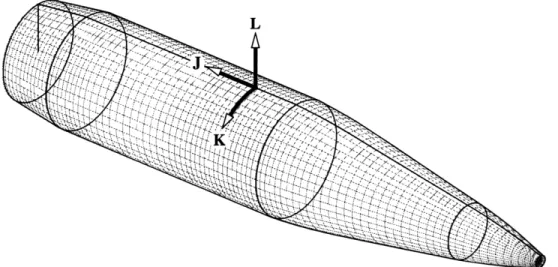
The axisymmetric body of revolution, which forms the foundation of all the config-urations evaluated, can be gridded quit easily by discretizing the profile shape and revolving it one complete turn or one half turn, depending on whether a full three-dimensional calculation will be performed or a calculation assuming lateral mirror symmetry. The surface discontinuities will be provided for naturally by placing a grid point on the profile at the discontinuity location. This process will result in a grid with an axis singularity at the center of the fuze tip and at the center of the base where the mapping will not be one-to-one. These grid singularities are accept-able within the OVERFLOW solver suite and are treated by first order extrapolation. Figure 2-1 shows an axisymmetric surface grid, defining the computational coordinate system.

Figure 2-1: Axisymmetric Surface Grid and Computational Coordinate System

The distribution of profile points is chosen such that all surface discontinuities are exactly represented by a grid point and such that there is a greater density of grid points in regions where high flow gradients are expected, which also happen to be near surface discontinuities, where shocks tend to form. The distribution is specified by use of weighting functions and the one dimensional physical-space weighted grid generator discussed in Appendix C. Grid dimensions are written JD x KD x LD, where JD is the number of longitudinal points, KD is the number of circumferential

points and LD is the number of points in the surface normal direction.

Sliced Configurations

It is not possible to represent exactly a sliced configuration with a single grid. This difficulty arises from the discontinuity line defined by the intersection of the body of revolution with the slicing plane. The discontinuity line is itself closed, making it impossible to work into a single grid. Thus, multiple overlapped grids are required to accurately describe this region. To simplify, grid development for blunt nose geome-tries has been foregone.

(a) Edge Grid Approximate Edge

(c) Overlapped Grid System

Figure 2-2: Component and Resultant Grids for Sliced Geometry

Figure 2-2 shows the individual and overlapped grids for the sliced configuration. As the figure shows, the slice is decomposed into a deformed body of revolution grid and an edge grid. The deformation was performed by projecting grid points from the

nominal body of revolution grid onto the slice plane. For the half-plane above the axis of revolution, the points are simply dropped straight down onto the slice plane. The nominal grid points lie on a circular arc which is at most a half-circle so that the projection is one-to-one, that is, the new set of points has no folds. For the half-plane below the axis of revolution, the circular arc of nominal grid points is more than a half-circle and the nominal grid points are transformed to lie on a half-circle whose diameter is equal to the width of the slice at that location before being project onto the slice plane. The edge grid defines the intersection of the slice plane and the body of revolution exactly (acting as a seam grid). The grid is marched away from the edge and projected onto the surface.

The underlying deformed body of revolution has several abnormalities which sug-gest that it would be unsuitable for use as a single grid. First, some quadrilaterals get wrapped around the edge, such that one side lies on the slice plane and one corner of the opposing side lies on the body of revolution. These quadrilaterals are ill-defined in that the surface normals defined by triangular decomposition are discrepant. Second, the projection process and transformation described in the previous paragraph results in high stretching close to the singular axis point. The first circumferential plane of cells away from the axis degenerate into triangles (as the axis condition necessitates), but the ellipsoidal shape of the slice intersection skews the cells more than would be desired. Both of these abnormalities are concealed by the edge grid, which results in an overlapped grid system that is well defined.

Despite the seeming inappropriateness of the underlying deformed body of revo-lution, the flow solver was found to be robust to the abnormalities under the whole Mach range of interest. A comparison was made with the overlapped grid predictions and was found to be in good agreement, which made it a cost effective alternative for the design investigations.

Bent Configuration

The so-called bent configuration is generated by linearly shearing an axisymmetric surface grid to produce an approximation to a deflection type bending. Actuated

mechanisms for bending would most likely pivot the fuze section, such that the arc length, shape of the cross-sections (constant x, for example) and orientation of the blunt nose would differ from the geometry evaluated here.

Strakes

A single strake geometry is explored for design purposes. The geometry was chosen to simplify grid topology, but was conceived to be aerodynamically representative of the concept. Figure 2-3 depicts the geometry of a strake, as defined by a single grid. The viscous surface lies entirely on one computational plane. Again, the strake geometry and grid topology are chosen such that grid lines naturally define surface discontinuities. The grid could be improved by relaxing the lateral spacing in the surface overlap region, causing the grid to splay out laterally, but it was found that the connectivity was reasonable.

K

(a) Grid Topology

Figure 2-3: Strake Grid T

2.2.3

Volume Grid Generation

(b) Actual Grid opology and Geometry

Once the surface grids have been generated, the volume grids are generated by "grow-ing" the grid from the surface with the hyperbolic grid generator HYPGEN [5], which is part of the OVERFLOW flow solver suite. Figure 2-4 shows a symmetry plane of

a typical volume grid. The volume has three regions: a surface region, a near field region and a far field region. These three regions are characterized by their grid spac-ing normal to the surface. The surface region has the highest density of grid points and thus contains the majority of the grid points. The wall spacing must be sufficient

: to capture the boundary layer velocity profile, as modeled by the turbulence model.

For the Baldwin-Barth [2] turbulence model employed, the wall spacing should be about y+ = 1, which was achieved in most configurations and flow conditions with a non-dimensional wall spacing of 10-6. The near field region allows for greater grid res-olution of the inviscid flow response to the displacement body. The relative sparseness of the far field region results from the smaller disturbances and milder flow gradients present in this region. The far field boundary was placed twenty reference lengths away from the surface to allow sufficient volume for dilation of transonic flow fields.

Figure 2-4: Half-Plane Showing Structured Volume Grid

2.2.4

Overlapped Connectivity

After all the volume grids have been generated, connectivity between the grids is calculated with PEGSUS [41]. Calculating overlapped grid connectivity is the process

of searching for the best interpolation stencil for each grid point in an overlapped region. An interpolation stencil consists of grid points from other grids and requisite weightings with which to perform tri-linear (linear three-dimensional) interpolation. Interpolation is the mechanism by which information is passed between the aggregate of grids.

The details of particular methods employed by PEGSUS will not be discussed, but the two requirements for good connectivity will be noted. First, there must be at least three cells overlap between adjacent grids. Second, the overlapping cell volumes must be similar. Quality of the connectivity is measured by how well balanced the interpo-lation stencils are in spatial configuration. In practice, reasonable connectivity can be obtain despite a region of disparate cell sizes, if they are well oriented. Furthermore, the coarser grid must be capable of adequately resolving the flow gradients.

2.3

Numerical Convergence

Numerical solutions must converge spatially as the density of grid points increases, and iteratively has the solution progresses towards steady-state, be it a constant or a limit cycle.

2.3.1

Spatial Convergence

Numerical discretization of complex flow fields usually result in approximations of

second order accuracy in the discrete spacing, written O (Ax2, Ay2, Az2, At2), due

to the truncation of the Taylor series approximation of the derivatives. Consistency requirements necessitate that truncation error tends towards zero as the spacing tends towards zero. Thus, the approximate solution should converge to the exact solution as the grid resolution increases. Grid resolution must be increased until the change in the predicted quantities becomes sufficiently small, at which point the grid is said to be converged.

The variations of the coefficients with grid spacing in the two orthogonal surface directions are given in Figure 2-5. Longitudinal calculations were performed with

- - - - %ACA, Mach 1.1, =4 -- - - %ACA, Mach 1.1, a=4*

%ACN, Mach 1.1, a=4 %ACN, Mach 1.1, a=4°

15 --- %ACm, Mach 1.1, ac=4 10 -.. --- %ACm, Mach 1.1, a=4'

- - - - %ACA, Mach 0.90, a=4 - - - - %ACA, Mach 0.90, a=4

%ACN, Mach 0.90, a=4 - %ACN, Mach 0.90, a=4*

10 %ACm, Mach 0.90, a=4° - - - %AC, Mach 0.90, a=4

& z

:.. -- , _{,, I.}

0.002 0.004 0.006 .oa 0.01 0 0.05 0.01 0.015 0.02 0.025 0.03 0.035 0.04

1/JD 1/KD

(a) Longitudinal Spacing (b) Circumferential Spacing Figure 2-5: Spatial Convergence in Two Orthogonal Surface Directions

43 circumferential grid points and 100, 150 and 300 points longitudinally. Circum-ferential calculations were performed with 150 longitudinal points and 24, 42 and 83 points circumferentially. The force and moment coefficients generally tend to converge quadratically, as the error in numerical accuracy does, but there are some exceptions due to nonlinear changes in the flow field. Longitudinal refinement results in a decrease in the axial force, while circumferential refinement results in an increase. Similarly, longitudinal refinement results in an increase in pitching moment, while cir-cumferential refinement results in a decrease, although pitching moment appears to be only weakly dependent on circumferential spacing for higher Mach numbers.

In practice, properly converged grids may not be used because the cost will impede the effectiveness of the computational model in the design process. Such cost saving measures must be used with good judgment and experience with the geometry at hand because the formulation of numerical approximations does not guarantee well behaved degradation of accuracy for grids far from being converged. Engineers often also utilize an intuitive but usually unrigorous principle that approximations will give fair predictions of trends, even when the predicted magnitudes are poor. With experience, poorly resolved grids can be useful during preliminary design studies for finding trends and approximate locations of maxima. The use of such lower order

44

approximations can be limited because shock locations and separation behavior are both strongly influenced by grid resolution and often have a strong influence on the solution.

2.3.2

Temporal Convergence

Steady-state solutions utilize local time step scaling for convergence acceleration. Typically, both a time step and a minimum required CFL are specified. Thus, as the time step is decreased a value will be reached below which the minimum CFL

specified wholly determines the local time step. Increasing the CFL number in the outer field can abet solution convergence by accelerating the establishment of the outer inviscid flow which is often a strong driver of the viscous boundary layer region. Time steps are determined by first attempting to use a time step of 1.0, then decreasing the time step an order of magnitude for subsequent attempts until the solution stabilizes. For well behaved steady-state solutions on moderate grid resolu-tions (150 x 43 x 60) it was found that a time step of 0.1 and a minimum CFL of 5.0 produces stabile solutions for Mach 0.80 to about Mach 1.1 or so. Higher Mach numbers required a time step of 0.01 and a minimum CFL of 2.0.

Time accurate solutions require a time step small enough to resolve the time de-pendent flow behavior and to maintain numerical stability. Transonic Mach numbers, near Mach 0.90, were found to converge for a time step of 0.001 for non spinning cases. Time accurate solutions with moving shocks require the use of the computationally more expensive block tridiagonal implicit factorization of the left hand side, as dis-cussed in Appendix B, further increasing the cost. Both the ARC3D diagonalized form and the block tridiagonal were used to compute unsteady transonic solutions and were found to give identical predictions, being equally accurate in modeling the recirculating base flow which is responsible for the unsteadiness.

Maximum allowable time steps for both steady-state and time accurate calcula-tions depend on grid quality and resolution as well as on the physical time scales of the flow problem. Grids of poor quality, containing skewed or highly stretched cells, can destabilize a solution requiring smaller time steps. Time steps must also be

reduced for fine meshes adding additional cost to solution refinement by increasing not only the per iteration cost from additional grid points, but by also increasing the number of iterations required.

Grid refinement in the boattail and wake regions tends to adversely affect solution convergence for transonic Mach numbers. Solutions often do not converge to constant values, but develop limit cycles. Coarser grids damp inherent physical unsteadiness and stabilize the solution, but may not yield accurate results. Validation studies show that the chosen grid resolutions have sufficient accuracy for preliminary design studies. Both fine grids and the spinning boundary condition discussed below were found to exacerbate unsteadiness at transonic Mach numbers and required time accurate time stepping.

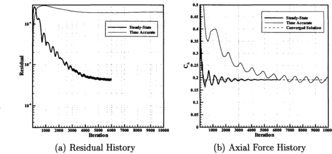
Figure 2-6 compares two temporal convergence histories, both at Mach 0.91 and

40 angle of attack. The steady state solutions has been computed on a 150 x 43 x 60 point grid, while the time accurate has been computed on a 300 x 43 x 60 point grid. The time accurate time stepping was necessary for the higher resolution grid because steady-state time stepping did not converge to a solution. Notice that the two methods of time stepping converge close to the same average solution, adding confidence to the numerically stabilized solution obtained from coarser grids.

0.45 - Steady-State

10 - Time Accurate

Steady-State 0.4 - - - - - Converged Solution

Time Accuate

0.35

• .. : 0.2 5_0.3

0.15

10.01