Control of nonlinear systems represented in quasilinear form

CONTROL OF NONLINEAR SYSTEMS

REPRESENTED IN QUASILINEAR

FORM

Josef Adriaan Coetsee

B.Sc.(Hons) Elek. Rand Afrikaans University, 1979

S.M. Aeronautics and Astronautics Massachusetts Institute of Technology, 1985 SUBMITTED TO THE DEPARTMENT OF

AERONAUTICS AND ASTRONAUTICS IN PARTIAL FULFILLMENT OF THE REQUIREMENTS FOR THE DEGREE OF

Doctor of Philosophy

in Aeronautics and Astronautics at the

Massachusetts Institute of Technology February 1994

@ Massachusetts Institute of Technology 1994. All rights reserved.

Signature of Author ... Certified by ... Certified by ... Certified by ... Certified by ...

S

De - Aeronautics And Astronautics

, , Dece;nber 17, 1993

Prof. W.E. Vander Velde, Thesis Supervisor Department of Aeronautics 4nd Astronautics

Dr. H. Alexander, Thesis Committee Member Senior Engineer, Orbital Scieresy Co/poration

Prof. J-J.E. 3Sotine, Thesis Committee Member D,,partment of Mechanical Engineering

Dr. A. Von Flotow, Thesis Committee Member , President, Hoof Technology Corporation

Accepted by... ,,,,, ,,,,

T-rr i Ipi

tE- I ( 1J4j

' f. Harold Y. Wachman, Chairman Department Graduate Committee

CONTROL OF NONLINEAR SYSTEMS REPRESENTED

IN QUASILINEAR FORM

by

Josef Adriaan Coetsee

Submitted to the Department of Aeronautics And Astronautics on December 17, 1993, in partial fulfillment of the

requirements for the degree of

Doctor of Philosophy in Aeronautics and Astronautics

Abstract

Methods to synthesize controllers for nonlinear systems are developed by exploiting the fact that under mild differentiability conditions, systems of the form:

5

=

f(x) + G(x)u

can be represented in quasilinear form, viz:

c = A(x)x + B(x)u

Two classes of control methods are investigated:

* zero-look-ahead control, where the control input depends only on the current

val-ues of A(x), B(x). For this case the control input is computed by continuously solving a matrix Ricatti equation as the system progresses along a trajectory.

* controllers with look-ahead, where the control input depends on the future

be-havior of A(x), B(x). These controllers use the similarity between quasilinear systems, and linear time varying systems to find approximate solutions to op-timal control type problems.

The methods that are developed are not guaranteed to be globally stable. However in simulation studies they were found to be useful alternatives for synthesizing control laws for a general class of nonlinear systems.

Prof. W.E. Vander Velde, Thesis Supervisor Department of Aeronautics and Astronautics

Acknowledgments

I must first of all thank my wife and children for their support and the patience they have shown during the past few years. I also have to thank my parents, and my parents in law, for their very generous support and encouragement. Without them this endeavor would not have been possible.

Further thanks are due to my supervisor, Prof. Vander Velde. I can only speak in glowing terms of my experience of working with Prof. Vander Velde - he is a wonderful role model, both academically and personally. I also have to thank the other members of my doctoral committee, they have provided me with keen insights, advice and friendly support throughout.

This work conducted with support provided by NASA Langley under NASA Research Grant NAG-1-126.

Contents

1 Introduction

1.1 Feedback Linearization of Nonlinear Systems . . . . 1.1.1 Global Feedback Linearization . ...

1.1.2 Partial Feedback Linearization and Normal Forms . 1.2 Optim al Control ...

1.3 O verview . . . .

2 Quasilinear Description

2.1 Generality of the Quasilinear Form . ... 2.2 _{Quasilinear Form for Mechanical Systems ...}

2.3 Stability Analysis Using the Properties of A(x) . . . . 2.3.1 Stability Analysis Based on Eigenstructure of A(x) 2.3.2 _{Stability Analysis via Matrix Measure Theorems} . . 2.4 Sum m ary . . . .

3 Quasilinear Controllers with Zero Look-ahead

15 21 .. . 24 S. . 33 . . . 34 S. . 39 .. . 45

3.1 Introduction . . . . 3.2 The Continuous Ricatti Design Method . . . .

3.2.1 The H-J-B-Equation and Quasilinear Dynamics ... 3.2.2 The Continuous Ricatti Design Feedback Law ... 3.2.3 Controllers for Combined Tracking and Regulation ... 3.3 Stability Analysis ...

3.3.1 Local Stability Properties ...

3.3.2 Single Equilibrium Point at the Origin . ...

3.3.3 Non-local Stability Analysis via Linear Time Varying Regulator Theory ...

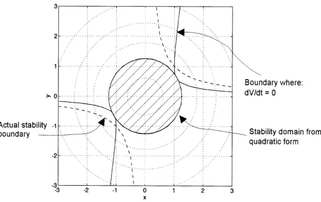
3.4 Stability Region Assessment . ...

3.4.1 Stability Domain Assessment Using Quadratic Forms ... 3.4.2 Stability Domain Assessment using Zubov's Method . 3.5 Computational Issues . ...

3.5.1 Eigenvector Method ... 3.5.2 Schur-vector Method . ... 3.5.3 Kleinman's Method . ...

3.5.4 Collar and Jahn's Method . . . . 3.5.5 Recommendation . . . . . 3.6 Simulation Results ... 3.6.1 System Dynamics . . . . . . . . . . 102 . . . . 103 103 46 . . . . . . 47 . . . . . 84 101

3.7 Summary ...

4 Controllers with Look-Ahead

4.1 Introduction .. .. . . .. . .. .. .. . . .. .. 4.2 Short Term Optimal Tracking . . . . 4.3 Receding Horizon Control . . . . 4.4 Long Term Optimal Control . . . . 4.5 Look-Ahead Control Using the Quasi-Linear Form

4.5.1 Introduction ...

4.5.2 The Look-ahead Issue . . . . 4.5.3 Implementing the Look-ahead Controllers 4.6 Simulation Results . . . . 4.7 Sum m ary . .. .. . . .. ... .. .. .. .. ..

5 Control of Flexible Manipulators

5.1 Introduction . . 5.2 System Dynamics 5.3 Simulation Results 5.4 Summary ... . . . . . 145 146 . . . . 150 . . . . 158 6 Conclusions 6.1 Future Work . . . . 113 113 115 118 126 128 128 131 132 137 141 145 160 162 108

A Modeling and Automatic Generation of Equations of Motion using Maple

A.1 Overview ... A.2 Dynamics Model ...

A.2.1 Notation .. . . . A.2.2 Axis systems .. . . . A.2.3 Kinetic energy .. . . . A.2.4 Potential Energy . . . A.2.5 Equations of Motion . A.3 Using the Routines .. . . . . A.4 Description of routines used .

A.5 Foreshortening .. . . .

A.6 Example of "template.mpl" . A.7 Annotated Example of Session

164 164 165 . . . . . 167 . .. 168 . .. 170 ... 177 . . . 179 180 182 183 185 . . . . 18 7

List of Figures

2-1 Double Pendulum ...

2-2 Nonlinear Spring Mass Damper . ...

3-1 Phase Plane Plot for Linear Feedback . ... 3-2 Phase Plane Plot for Continuous Ricatti Design . ... 3-3 Block Diagram of Augmented System with Integral Control ... 3-4 Stability Domain Using Quadratic Form . ... 3-5 Standard Grid for Finite Difference Method . ... 3-6 Solution Strips for Zubov's P.D.E . ...

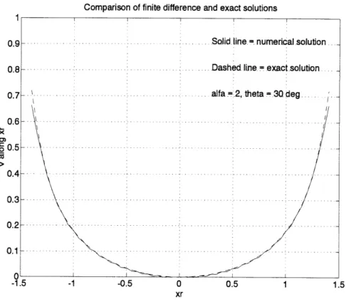
3-7 Exact vs. Finite Difference Solution to Zubov's P.D.E . ...

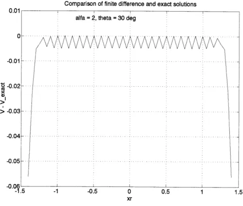
3-8 Error between Exact and Finite Difference Solutions to Zubov's P.D.E. 3-9 Exact vs. Finite Difference Solution to Zubov's P.D.E. - o large . . 3-10 Exact vs. Finite Difference Solution to Zubov's P.D.E. o small .

3-11 One Link Arm ... .. . ... 104 3-12 Stable Response - Continuous Ricatti Design . . . . 109

3-13 Unstable Response Linearized Design ...

3-14 Unstable Response - Continuous Ricatti Design . . . .

4-1 Time Intervals for Short Term Tracker . . . . 4-2 Responses for Short Term Tracker . . . . 4-3 Responses for Receding Horizon Tracker . . . . 4-4 Responses for Long Term Look-ahead Controller . . . .

5-1 Two Link Flexible Manipulator . . . . 5-2 Flexible Manipulator Maneuver . . . . 5-3 Two Link Flexible Manipulator Responses - Linearized Design

5-4 Two Link Flexible Manipulator Responses - Continuous Ricatti Design 156 5-5 Two Link Flexible Manipulator Responses - Long-term Look-ahead .

A-1 Coordinate Systems for General Planar Flexible Manipulator . . . . 166 A-2 Model of joint at the root of link i

A-3 Foreshortening . . . . 110 111 115 140 142 143 148 154 155 159 171 185

List of Tables

Chapter 1

Introduction

Control engineering has played an important role in the development of industrial society. One of the earliest applications of control devices can be found in Watt's use of flyball governors to control the speed of steam engines [42]. Subsequently the discipline has undergone a great deal of theoretical development and has found practical application in a wide variety of systems such as the control of chemical processes, robotic manipulators, flight vehicles etc.

To develop control systems the following paradigm is often used:

1. It is assumed that there is a requirement for a system, also referred to as the plant, to behave in accordance with certain specifications. For example the requirement may be for a motor (the plant) to operate at a certain speed. 2. When the system's natural behavior does not in itself meet the requirements, it

may be necessary to use some control inputs to induce the desired behavior. As an example some "regulator" may be required to ensure that a motor operates at the required speed.

3. The next step is to obtain an abstract dynamical model for the system. Usually it is assumed that the system's behavior is adequately described by a set of

ordinary differential equations. The differential equations are often derived on the basis of some physical principles, but other approaches are possible. For example it can simply be assumed that the system dynamics are described by a generic set of differential equations with unknown parameters. In this case the parameters in the dynamical model may be adjusted to ensure that the model reproduces available empirical data through a process of system identification. Alternatively the controller may be designed in such a way that it can cope with the uncertainty in the parameter values.

4. Once the dynamical model of the plant is available, one develops (usually by analytical means) a control law that will modify the plant's behavior to be in line with the original requirements.

5. Finally the controllers are implemented and tested to ensure that the overall requirements are met.

Much of control theory has been concerned with step 4, i.e. the synthesis of control laws. Ideally synthesis methods should:

* be generic (i.e. can be applied in a straightforward fashion to most systems), * provide the designer with a convenient way to adjust the system's response, and

* guarantee stable system behavior.

Many design methods have been developed and these mostly meet the objectives above, depending on the control objectives and also the class of system that is to be controlled. We can make the following broad (but not exhaustive) classification:

A. Class of system:

- Linear time invariant systems: i.e. systems with dynamics of the form:

where x is the state vector and u is the set of control inputs.

- Linear time varying systems: i.e. systems with dynamics of the form:

c = A(t)x + B(t)u _(1.2)

Here the matrices A(t), B(t) are known functions of time.

- Nonlinear systems: these are typically systems of the form:

X = f(x,u), or

x

(1.3) (1.4)

Within the class of nonlinear systems there exists a special class of systems, i.e. globally feedback linearizable systems. These systems are relatively easy to control - see Section 1.1.1 for more details.

- _{Nonlinear time-varying systems: i.e. systems with dynamics of the form:}

5 = f(x, u, t) (1.5)

B. Control objective:

- Stabilization: Here the only objective is to find a control law that ensures

that the system is (globally) stable.

- Optimization: Here the objective is to find some control

mizes a cost function which typically has the form:

input that

mini-J = xT(tf)Hx(tf) + f(xTQx + uTRu)dv _(1.6)

(It is implicitly assumed that part of the control objective is to ensure that the system remains stable)

- Adaptive Control: In this case it is typically assumed that the system

the designer, for example:

x = f(x, p, u) (1.7)

The controller then adjusts itself to accommodate the unknown parameters

p and still maintain overall stability.

- Robust control: Any of the above cases becomes a robust control problem

if the objective is to maintain stability and performance objectives, de-spite the fact that assumptions regarding the nominal plant model may be incorrect.

- _{Stochastic control: If the system dynamics in any of the cases above are}

affected by a random process we have a stochastic control problem. An example would be the following linear time varying system that is driven by a random process w:

x = A(t)x + B(t)u + rw (1.8)

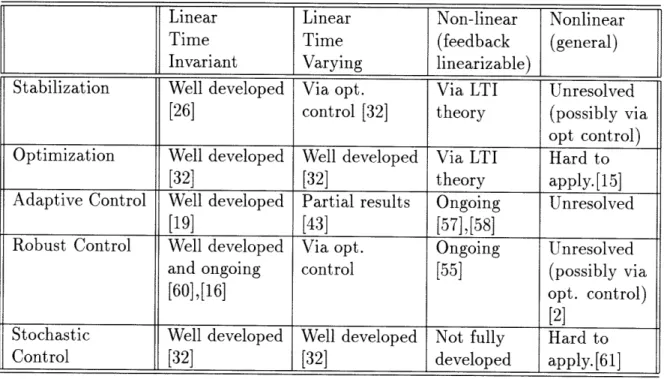
Table 1.1 gives a (very) brief summary of the availability of synthesis methods for different control problems. We note that the control of general nonlinear systems that are not feedback linearizable remains a very difficult problem.

Our investigations will mostly be concerned with developing a synthesis method for general nonlinear systems which are not feedback linearizable. Since the global feed-back linearization theory also illuminates the general nature of the problem we want to address, we will start by examining it. Following that, we will briefly discuss op-timal control as an approach to synthesize control laws for nonlinear systems and then finally in Section 1.3 provide an overview of the methods to be developed in this thesis.

Linear Linear Non-linear Nonlinear

Time Time (feedback (general)

Invariant Varying linearizable)

Stabilization Well developed Via opt. Via LTI Unresolved [26] control [32] theory (possibly via

opt control) Optimization _{Well developed Well developed Via LTI Hard to}

[32] [32] theory apply.[15]

Adaptive Control Well developed Partial results Ongoing Unresolved

[19] [43] [57],[58]

Robust Control Well developed Via opt. Ongoing Unresolved and ongoing control [55] (possibly via

[60],[16] _{opt. control)}

[2]

Stochastic _{Well developed Well developed Not fully Hard to}

Control [32] [32] developed apply. [61]

Table 1.1: Availability of Synthesis Methods

1.1

_{Feedback Linearization of Nonlinear Systems}

Global feedback linearization and normal forms for nonlinear systems are concepts that have recently been developed and provide much insight into the fundamental issues regarding the control of nonlinear systems. These concepts have their origins in work done by Krener [31] and Brockett [7] among others. Further developments in the theory were provided by Hirschorn [22], Jacubczyk and Respondek [25] as well as Hunt, Su and Meyer [23]. In discussing these ideas we will focus on single-input single-output systems, although the concepts can be generalized for multivariable systems (see e.g. Slotine and Li [59]).

1.1.1

Global Feedback Linearization

We first consider systems which are so-called globally feedback linearizable. Such sys-tems are relatively easy to control since, in the words of Brockett, they are "... linear

systems in disguise ... ". More precisely the system:

5C = f(x)+ g(x)u _(1.9)

is considered to be globally feedback linearizable if a combination of coordinate change:

z

= (x)

and feedback:

u= a(x) + /(x)v

applied to (1.9) results in the linear time-invariant system:

z

=

0 1 0 ...

0 0

0 0 1 ... 0 0

. 0 1 0 0 0 ... 0 0 for all x. Technically it is required that:

* the transformation:

z

=

c(x)

be a diffeomorphism, i.e. p(.) must be smooth, and its inverse -l(.) must exist, and also be smooth.

* the functions f(x) and g(x) be smooth.

For a system of the type given in equation (1.9), precise conditions exist for us to determine whether a system is globally feedback linearizable or not (see e.g. Slotine (1.11)

where:

(1.12)

(1.13)

and Li [59], or Isidori [24]). In order to state these conditions compactly we use the following standard notation and definitions (see e.g. Slotine and Li [59]). Let h(x) be a smooth scalar valued function, and f(x) and g(x) be smooth vector valued functions of the n-dimensional vector x.

* The gradient of h w.r.t x-coordinates is:

Vh Oh axl Oh aX2 Oh 8zn (1.15)

* The Jacobian of f w.r.t to x-coordinates is:

Vf

-(V fi)T

(Vf2)T

(Vfn)T

(1.16)

* The Lie-derivative of h w.r.t. f is given by:

Lfh =- (Vh)Tf

and higher order Lie-derivatives are defined as:

Loh = h

L'h = LfL-lh

* The Lie-bracket of f and g is given by:

adfg - [f,g] -Vg f - Vf g (1.17) (1.18) (1.19) (1.20) (1.21)

and higher order Lie-brackets are found from:

adog = g (1.22)

adg = [f,ad-'g] (1.23)

* A linearly independent set of vector fields {fi, f2,... ,f} is said to be involutive

if and only if there exist scalar functions aijk(X) such that:

m

[fi,fj] = aijk (x)fk(x) Vi,j (1.24)

k=1

With the definitions above, the necessary and sufficient conditions for feedback lin-earizability of (1.9) can be compactly stated. We have the following powerful theorem (see e.g. Slotine and Li [59] for details):

Theorem 1.1.1 The nonlinear system (1.9) is globally feedback linearizable if and

only if the following conditions hold for all x:

* The vector fields

{g, adfg,..., ad-1g} (1.25)

are linearly independent. * The vector fields

{g, adfg,..., ad-2g} (1.26) are involutive.

In proving the theorem above one also obtains a method to construct the coordi-nate transform and feedback law required to put (1.9) into the linear form of equa-tions (1.12) and (1.13). The construction, which we describe next, requires one to solve a potentially difficult set of partial differential equations.

Assuming that conditions (1.25) and (1.26) are satisfied, the process to feedback linearize the system will be:

1. Solve the following set of p.d.e's for i1l:

VT ad'g = 0 i

Vi adf -g # 0

2. Apply the coordinate transform:

z = cp (x) =

which will result in the following dynamics:

Z1 z2 (1.27) (1.28) JfC1 rn-1 y01 Z2 Z3

+ #(z)u

a(p(x))

(W,(x))

We shall refer to (1.30) as the cascade canonical form1 _{because the system is}

now made up of a string of integrators with the highest derivative driven by a nonlinear function of the state as well as the control input.

1The author is not aware of a standard term used for this canonical form for nonlinear systems = 0,...,n-2

3. Apply the feedback:

1

u = (-a(p(x)) + v) (1.33)

Once we have applied the feedback and transformations above we can apply the large body of control theory for linear systems. However the process outlined above is easier stated than applied. Difficulties arise on the following counts:

1. Establishing that a system is globally feedback linearizable (so that we know that the p.d.e's (1.28) have a solution) can require significant effort. For in-stance, if we cannot analytically check the conditions of Theorem 1.1.1, we have to test these conditions numerically at "every" point in the state space. 2. We have to solve the partial differential equations (1.28) which may be a far

from trivial problem to do either analytically or numerically.

3. Once we have applied "inner loop" control (1.33), we expect to apply further state feedback control to get the L.T.I. system to behave appropriately, e.g.:

I = kTz (1.34)

= k, kk₂ ..., k LpL (1.35)

For both the case where we can find z = p(x) analytically as well as the case where we find P1 numerically, the feedback law might be quite sensitive to

errors in x. Since the "outer loop" feedback, v = kTz, involves derivatives of 1i we would expect any problems to be exacerbated if we have to find P1 by numerically solving the p.d.e.'s (1.28).

1.1.2

Partial Feedback Linearization and Normal Forms

In the previous section we outlined the situation where a system can be globally feed-back linearized. As we might expect, there exists a large class of systems which cannot be feedback linearized, and thus remain difficult to control. To better understand the issues involved the concept of partial feedback linearization will be examined next. We shall see that if f(x) and g(x) are smooth enough, systems of the form (1.9) can be (locally) partially feedback linearized and put in a normal form.

Consider controllable systems of the form:

5C = f(x) + g(x)u (1.36)

y = h(x) (1.37)

where y = h(x) is an arbitrary smooth function of the system state. Usually y will be

some output variable that we want to control. In its simplest form partial feedback linearization is achieved as follows: We successively differentiate y until the control input appears in the expression for say the rth derivative of y, viz:

dy_

a

dr-dtr -

x

= Lih + LgL-h (1.39)

- (x) + 3(x)u _(1.40)

The state equations for the system can then be written as:

Yl Y2

Y2 Y3

S (1.41)

r a(x) + P(x)u

If r = n, where n = is the dimension of the state vector, and we use the control: 1

u= (-a(x) + v) (1.42)

we have globally feedback linearized the system. The process for global feedback linearization can thus be thought of as a method to appropriately construct y = h(x), so that r = n, if it is at all possible. Furthermore, the conditions of Theorem 1.1.1 can then be thought of as tests to determine whether a suitable h(x) can be found. In equation (1.41) we see that O(x, u) depends on both x and u. It can be shown that using an appropriate transformation (which is also constructed by solving partial differential equations) the system can be put in the following normal form:

Yl Y2

Y2 Y3

(1.43) r a(yq, r) + (y, rl)u

i7 w(y, rl)

This normal form enables us to better understand what we can achieve in controlling the system. For instance, if ((y, t7) / 0 Vx, we can fully determine the input-output relation between u and y. However, since y acts as an input to the q states, we see that y following a certain trajectory forces a specific behavior for the internal dynamics:

77 = w(y, r) (1.44)

Clearly it is possible that the states 77, which are not observable via h(x), can become unstable, depending on the y trajectory.

An important special case occurs when y - 0. The dynamics of (1.43) subject to the constraint y E 0 are called zero-dynamics [59] of the system. In terms of the normal

form we get:

0 (1.45)

If the zero-dynamics of the system is asymptotically stable the nonlinear system is said to be asymptotically minimum phase. It can be shown that this definition captures our standard understanding of minimum-phase systems for the case where we are dealing with linear systems (see Slotine and Li [59]).

At this point it becomes clear what the challenge is regarding the control of nonlinear systems. Typically the problem will be to obtain certain desirable behavior from our output variable y while still maintaining stability of the internal dynamics.

1.2

Optimal Control

Another approach to synthesizing controllers for nonlinear systems is to find the control input through solving an optimal control problem. In principle this approach meets all our objectives for an ideal synthesis method. For example if our objective is to stabilize a nonlinear system of the form:

c = f(x, u) with equilibrium point: (1.46)

0 = f(0,0) (1.47)

We then pose an optimization problem which has the objective to minimize the fol-lowing cost function:

J = (xTQx + uTRu)d (1.48) where we assume that both

Q

to the origin from any initial condition. If we apply this control input to the system we will incur a certain finite cost, say J,(xo). Furthermore if we apply the optimal control input to the system there will be a certain associated cost, say J(xo) which has to be less than Jo and thus finite. Now note that since

Q

A further attractive aspect of the optimal control approach is that it provides us with a method to conveniently adjust the system responses by adjusting the cost function. The only undesirable feature of the optimal control approach is that it is compu-tationally very demanding. If the goal is to obtain the optimal control as a state feedback law we have to solve a nonlinear partial differential equation, the Hamilton-Jacobi-Bellman equation , for the whole region of the state space where the system is to operate (see Section 3.2.1 for further discussion). Alternatively we have to find the optimal control input by numerically solving a two point boundary value problem [15].

1.3

Overview

As indicated earlier we will be mostly concerned with developing a controller synthesis method for nonlinear systems of the form:

5c = f(x)+ G(x)u (1.49)

We will exploit the fact (see Chapter 2) that provided f(x) meets certain smoothness requirements, equation (1.49) can be written in the following quasilinear form:

c = A(x)x + B(x)u (1.50)

com-puted by continuously solving a matrix Ricatti equation based on the instantaneous properties of A(x), B(x). We shall refer to this as a control law with zero-look-ahead. Related work appears in the thesis by Shamma [53] who investigates gain scheduling in the context of the LQG\LTR methodology [60], and takes a different perspective with regard to the stability issue.

In Chapter 4 we develop control laws that take into account the "future behavior" of A(x), B(x). We refer to these as control laws with look-ahead. The methods we investigate will all have underlying optimal control problems that have to be solved. By exploiting the quasilinear form we will obtain approximate solutions to these optimal control problems.

Finally in Chapter 5 we will apply the controller synthesis methods we developed to control a complex nonlinear system, i.e. a flexible robotic manipulator similar to the space shuttle Remote Manipulator System [20].

Chapter 2

Quasilinear Description

In this chapter we will examine some of the basic issues in dealing with nonlinear dynamical systems of the form:

x = A(x)x + B(x)u _(2.1)

We shall refer to such systems as quasilinear systems.

2.1

Generality of the Quasilinear Form

The following lemma from Vidyasagar [63] shows that under mild differentiability conditions, systems of the form:

5 = f(x) + G(x)u (2.2)

can always be transformed to the quasilinear form of equation (2.1). The lemma is more general than we will need since it caters for the case where f(O)

$

Lemma 2.1.1 Suppose f : R - Rn is continuously differentiable. Then there exists a continuous function A : R" -- R X" such that:

f(x) = f(O) + A(x)x, Vx E R" (2.3)

Proof:

Fix x and consider f(Ax) as a function of the scalar parameter A. Then

f(x) = f (0) + f(Ax) dA (2.4)

f(O) [+j Vxf(Ax) dA] x (2.5)

so that

A(x) -- Vxf(Ax) dA (2.6)

Q.E.D.

The above formula gives us a specific quasilinear form for any C' function f(x). Equation (2.6) is useful in cases where the quasilinear form may not be immediately apparent. For example let:

sin(x1 + X2) f(x) = in(x 2) (2.7) sin(z2) Equation (2.6) gives: sin(x +x₂) sin(xl ₊x₂) A(x)= ("1+"2) (1+2) (2.8) 0 sin(X2) X2

Note that, in general, the quasilinear form for a given function f(x) is not unique. In fact, we see that we can add any vector that is orthogonal to x, to any row of

alternative quasilinear form for f(x) is:

sin(xi + ₂) - kl2 sin(x + ₂) - kx X1

i

f(x) 1- +X'2 1 i+X2 (2.9)

-k2X ₂ sin(2 k2Xl X2

X2

This non-uniqueness can be exploited as we shall see in Section 2.3.2.

2.2

Quasilinear Form for Mechanical Systems

In this section we will show that the equations of motion of a class of mechanical systems which operate in the absence of gravity can be put into quasilinear form without solving the potentially difficult integrals of equation (2.6). (See also Ap-pendix A which describes a set of computer routines that utilize this approach to automatically derive quasilinear equations of motion for flexible manipulators.)

We will use Lagrange's equations. They are:

d OL &L

d ) -q = Qi, i = 1... n (2.10)

where:

n = the number of degrees of freedom in the system

qi = ith generalized coordinate

Qi

L=T-U

T = kinetic energy U = potential energy

If we can express the kinetic and potential energy of the system in the form:

T = 1 TH(q)q4 (2.11)

U= qTKq (2.12)

where:

qT = [qi, q2, ... , qn] is a vector of generalized coordinates H(q) = a generalized inertia matrix

K = a generalized stiffness matrix

then Lagrange's equations can be written in vector format as:

H4 + Hq - VqT + Kq = Q

where: Q = [Q1, Q2,., Q,]T is a vector of generalized forces, and:

VqT a T 9q

(9T aT

aTIT

so that the equations of

motion= can be expressed as: motion can be expressed as:

H4 + (H -

(2.18)

H(q)4 + C(q, q)q + Kq = Q

To get a state space description we furthermore assume that the system is controlled via the generalized forces and that they can be expressed as:

Q = M(q, 4)u

where the components of u are the control inputs to the system.

(2.13)

(2.14) (2.15)

(2.16)

desired state space form:

q

I

0

=t 0=I

I

+

S -H(q) - 1K -H(q)-'C(q, ) q H(q)-M(q, ) (2.20)

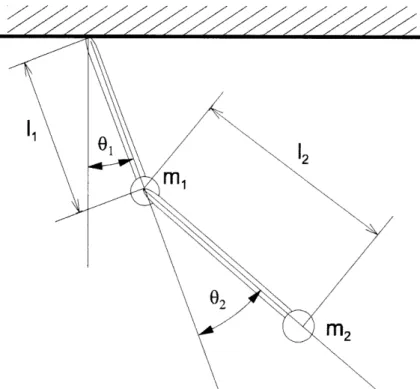
Note that the key to getting to the quasilinear form is to express the kinetic and potential energy as in equations (2.11) and (2.12). In the following example we shall use a double pendulum system to show how we can find the desired form for the kinetic and potential energy. We shall see that it is generally relatively easy to find the desired form for the kinetic energy. On the other hand, the expression for potential energy will only be in the desired form if we are dealing with the equivalent of "linear springs". This will typically be the case for flexible mechanical space based systems. If we are dealing with nonlinear "springs", e.g. gravity, we generally will have to use equation (2.6).

Example 2.2.1

Figure (2-1) shows a double pendulum with rigid massless links of lengths 11 and 12

respectively. The links also have tip masses m, and m2 and rotational springs K1

and K2 attached. For this system the generalized coordinates are 01 and 02, Viz:

q

I

02

We first find an expression for the kinetic energy. Let R₁ and R₂ be position vectors to each of the masses. Then kinetic energy of the system is given by:

T mi dR 1 dR 1 m2 (dR 2 dR2 (2.22)

2 dt dt 2 dt dt(2

with:

R

Figure 2-1: Double Pendulum as an integral over infinitesimal mass elements viz:

=f dR

T o dt

vol dt

R

dR

dt

For the double pendulum system we get:

d R

la

R

os(0

) 0

-I1 sin(01) - 12 sin(01 + 02) -12 sin(01 + 02)

J2(q) = = (2.28)

11 cos(01) + 12 COS(01 + 02) 12 COS(01 + 02)

Now we can express the kinetic energy in the desired form:

mT l TTJJt + M2qTJ J q (2.29)

- ilT [ImJTJ + m22TJ2] q

(2.30)

I 4TH(q)q _(2.31)

Next we find an expression for the potential energy. In the absence of gravity the potential energy of the system is given by:

Uspring = (K + K202) (2.32)

2q i K 2 q (2.33)

= qlTKq

(2.34)

which is of the desired form viz. equation (2.12). We achieved this form because we had linear springs. If we include the effects of gravity we will not be able to conveniently express the potential energy in the form of equation (2.12) - gravity does not act like a linear spring. Nevertheless we can still obtain a quasilinear form for our dynamics when gravity is present by e.g. using (2.6) as we shall now show. The potential energy due to gravity is given by:

Ugravity = -migli cos(01) - m 2g (11 cos(01) + 12 cos(0 1 + 92)) (2.35)

This gives rise to the following additional term in equation (2.13):

mlgll - mm2- 2g (-lI sin(01))- 12 sin(O1 + 02))

VqUgravity

(2.36)

In this case we can express the gravity term in quasilinear form as follows: (M l 1lln1 M1sin(0 m2 1+02) m2912 sin( 01+02 1 (milim21 1281 82) 2 81 82) VqUgravity = (01+02) (01 +0₂) (2.37) m292 sin( +02) _{m292 sin( 01+02)} 02 (01+02) (81 +2) - Ggrav(q)q (2.38)

We then get a result similar to equation (2.17):

Hq + (H- H(q)q q + [K + Grav(q)] q = 0 (2.39)

The rest of the process follows as outlined above. The resulting quasilinear equations of motion are given in Appendix B.

Remarks:

* The quasilinear form of equation (2.20) is already in a partially feedback lin-earized form, although not the normal form of (1.43). However, we are using "natural" coordinates, i.e. the variables of the equations of motion have physi-cal significance, whereas the variables r7 in the normal form of (1.43) usually do not have physical significance.

* If the number of actuators is equal to the number of degrees of freedom of the system, the quasilinear equations will be in the desirable cascade canonical form of equation (1.30). This will, for instance, be the case if we are dealing with robots with rigid links with actuators at each joint.

2.3

Stability Analysis Using the Properties of A(x)

In this section we will examine some stability tests for the ordinary differential equa-tion (o.d.e.):

that are based only on the properties of the matrix A(x). Because the o.d.e. (2.40) represents a very large class of nonlinear systems, viz. any o.d.e. 5C = f(x) with f(.) E C', we do not expect to find stability tests that are easy to apply and at the same time provide both necessary and sufficient conditions for stability. We note that the tests we discuss will also be useful for analyzing the stability of linear time varying systems where:

x = A(t)x (2.41)

2.3.1

Stability Analysis Based on Eigenstructure of A(x)

One is tempted to predict the stability of (2.40) based on the eigenvalues of A(x). We will show that the eigenvalues do not provide us with enough information to deduce stability and that we have to take into account the rate of change of the eigenstructure of A(x). The results we present are similar in spirit to other results regarding the stability of slowly varying systems (see e.g. [43],[63]).

We have

5c = A(x)x (2.42)

Assume that all the eigenvalues of A(x) are distinct, real and strictly negative. Then:

A(x) = T(x)A(x)T-l(x) (2.43)

where

T(x) = a matrix containing the eigenvectors of A(x)

A(x) = diag(Al(x), A2(x),..., A(x)) is a diagonal matrix containing the

We can then make the coordinate change:

z = T-1(x)x (2.44)

which results in the following dynamics for the transformed system:

z = T-(x)c + - (T-l(x)) x (2.45)

T-'A(x) (TT-1) x - T-1'TT-'x (2.46)

= A(z)z - (T-1(z)T(z)) z (2.47)

where for notational convenience we have not shown the state dependence of T in equation (2.46). To determine the stability of the system we use the following simple observation:

Fact 2.3.1 The system of o.d.e.'s:

z = A(z)z + M(z)z (2.48) A (z) 0 0 A2 (Z) 0 0 0 ... A(z) (2.49)

will be asymptotically stable provided that:

zTA(z)z + zTM(z)z < 0 Vz Z 0

Proof:

Use the candidate Lyapunov function:

(2.50)

V(z) = Iz z 2

with:

which is positive definite and radially unbounded. Then:

(2.52) (2.53) = zTA(z)z + zTM(z)z

and global asymptotic stability follows since V < 0 Vz / 0.

Q.E.D.

We can apply this fact to our case by noting that:

zTA(z)z -< z z

zTT-'(z)T(z)z _{< z||2 I T-'(z)T(z)z |2} S|T- 1(z)T(z) 12 zTZ

IlT-1(z)Tj(z)l 2 < v < C

ZTA(z)z + zTT-liTz < (- + V) zTZ < 0

That is if the rate of change of the eigenstructure is small enough, viz. T 0, we can infer stability pointwise from the eigenvalues of A(x). For example, consider the following seemingly complex second order nonlinear system:

= -(15 x9 ₃ + 1260 ₆ xX ₂ + 1890 ₇ XX ₁₂₂ + 1890 x x₂ +1260 x2X + 540 XX₂ + 135x x2 +135X ₂ 2+ 540 lX2 + 51 2 + 54x 1 + 15x X -6 x - 15x _{1 2} - 9x - 27 XX ₂ - 45 XX 2 and (2.54) so that if: (2.55) (2.56) we have: (2.57) (2.58) V = zTz

-33X x

4

+

+1260

+840

4

+

+

+

-

+364

+

+

+468x

+3502

These equations can be written in quasilinear form as:

c = A(x)x A(1, 1) = A(1, 2) = - {54 + 58 (x₁ + x2)2 + 18 (-2 x, - 3 x2)2 +18 (-2 x1 - 3X2)2 (X1 + X2)2 -6x 1 - 9X2 + 3 (-2x1 - 3X2) (x1 + X2)2 +15 (X1 + X2)6 + 15 (X1 + x2)8} / {1 + (x1 + 22)2} - {51 + 57 (x1 + X2)2 + 18 (-2 x1 - 3 2 )2 +18 (-2 x1 - 3x 2)2 (x1 + X2)2 -6 x1 - 9 x2 + 3 (-2 x1 - 3 x2) (x1 + x2)2 (2.59) (2.60) (2.61) (2.62) where

+15 (s1 + X 2)6 + 15 (X1 + X2)8 / 1 + (X 1 + 2)2} (2.63) A(2, 1) = {34 + 38 (x + X2)2 + 12 (-2 x, - 3X2)2 +12 (-2 x - 3 s2)2 (X + X2 )2 - 4 x1 - 6 X2 +2 (-2 xs - 3 X2) ( 1 + X2) 2 + 10 (x1 + X2)6 +10 (Xl + X2 )8} / {1 + (X₁ + X2)2} (2.64) A(2, 2) = {31 + 37 (sx + X2)2 + 12 (-2 xi - 3X2 )2 +12 (-2 xs - 3 s2)2 (1 + X2)2 - 4 sx -6 x2 + 2 (-2 xl - 3X2) (X + X2)2 + 10 (X1 + s2 )6 +10 (X1 + X2)8} / {1 + (X 1 + X2)2} (2.65)

For A(x) above, an eigenvector matrix is:

-1 -3/2 _(2.6)

Since eigenvectors are only uniquely determined up to a scale factor we use the fol-lowing (eigenvector) transformation matrix:

T = _(2.67)

where we assume that a and 3 are constants. For these eigenvectors the eigenvalues of A(x) are given by:

3+x2

+2xlX2

A1(X) = - 2 1 s2 s2 (2.68)

1+ r + 2xi x2 + 2

A2 () = -5 2 - 30 xX 2 - 75 2 1 2 2 1 2

Then upon applying the state transform:

and noting that T = 0 we get:

with: -(12 + O2z )/(4 + /2z2 )

A(z) =

We see that A I(z) < 0, A2(z) < 0 and also T = 0 and hence conclude that

is stable.

the system

2.3.2

Stability Analysis via Matrix Measure Theorems

Another approach to inferring stability of (2.40) from the properties of A(x) is to use the matrix measure or logarithmic derivative of A(x) which is given by:

Definition 2.3.1 Let A be an n x n matrix and 11. 1i be an induced norm on Rn_X

The corresponding matrix measure Iu(A) of the matrix A is given by:

(2.73)

p(A)= lim I+_C-*0+

The matrix measure was originally used to determine stability and error bounds for numerical integration methods [13] and later used by Coppel [12] to obtain solution bounds for linear time varying o.d.e.'s. Desoer and Haneda [14] also used matrix measures to bound solutions of o.d.e.'s, bound accumulated truncation errors for numerical integration schemes and determine convergence regions for the Newton-Raphson solutions of nonlinear equations. Further related work appears in [51], [52]

z = T-1x _(2.70)

z = A(z)z (2.71)

and [44].

The matrix measure is defined so as to easily bound the behavior of flx(t)l| for o.d.e.'s of the form:

x = A(x, t)x (2.74)

The following theorem shows how this is done.

Theorem 2.3.1 [63],[14] Consider the o.d.e.:

c = A(x,t)x, x E R' (2.75)

Let

H.H1

II.1

(2.76)

Suppose furthermore that there exist continuous functions a(t), 0(t) such that:

p(A(x, t)) < a(t), 3(t) < p (-A(x, t)) Vt > 0, Vx e R"

Ix(to)| exp (j -(r)dT)

<

Hx(t)ll

<

Proof:

We first show (2.76). We have from (2.75):

x(t + St)

=

I|x(t + 6t)|

= x(t) + A(x, t)x(t)St + o(St)

= [I + StA(x, t)] x(t) + o(St)

II [I + 6tA(x,t)]x(t)II + I|o(6t)H|

< |II + StA(x,t)l|H|x(t)ll + o(6t)jl

Then: (2.77) (2.78) (2.79) (2.80) (2.81) (2.82) d+ dt x(t)| < _{(A(x, t)) IIx(t) 1} dt

=

Ifx(t

+

St)|

- Ix(t)|

d+

d x(t)|

dt

S{IlI + 6tA(x,t)l, - 1} ||x(t)ll + o(6t)ll < lim III+ tA(x, t) |i - 1

(t)1

6t- o+ St

(2.83) (2.84) Equation (2.78) then follows by multiplying both sides of the inequality:

d+ dt < lim I+ 6tA(x, t) | - 1

"

m+t

_IIx(t)

" a(t)| x(t)|

with the integrating factor:

exp (- a(r)dT) (2.87)

Q.E.D.

The matrix measures associated with the 1, 2 and oc norms are given by:

|I

_+E

jot, n

IIX I12 ii1

-- 1l i(A) = max (ad

3 1 i;j

--+ 2(A) = Amx, (AT + A) /2

The usefulness of matrix measures becomes apparent by examining equations (2.77) and (2.78) and noting that y(A) can have negative values and thus be used e.g. to show that IIxII --+ 0. The following example shows how this can be done:

Example 2.3.1 Consider the following set of o.d.e.'s:

il -= -(3 + XlX2) 2 Xl + cos(xi) sin(x₂)x _{2 (2.91)} (2.92) 2 -- xi sin(x3) - X2 - 2x2 aiji) (2.88) (2.89) (2.90)

These can be put in quasilinear form as: x2 -(3+ x1X2)2 sin(xz ₎ cos(x) sin(Sx

1

For A(x) above we have:

Note that the quasilinear form is above is much more useful than

non-unique (see the alternative:

Section 2.1), and that the realization

-(3 + x X2) 2 sin(x ) - X₁ X₂

cos(xZ) sin(x2)

F

-2 X2

where now the -X lX2 term in A(2, 1) can become unbounded and thus make it

im-possible to establish the row or column dominance of the diagonal terms as required by equations (2.88) and (2.89)

Remarks:

* From equation (2.90) we see that the system (2.75) symmetric and negative definite.

will be stable if A(x) is

* Equations (2.88) and (2.89) show that in order to have p,(A(x)) < 0 (which we need for stability, see equation (2.78)) the diagonal terms of A(x) have to be negative and dominate the off-diagonal terms. Unfortunately, when dealing with physical systems we often naturally obtain dynamical equations that do not result in A(x) being diagonally dominant as we see in the following example and is also apparent in Section 2.2.

(2.93) pul(A(x)) P, (A(x)) <-1 (2.94) (2.95) :i2 (2.96)

m=1

g(x)

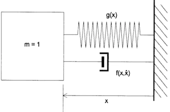
Figure 2-2: Nonlinear Spring Mass Damper

Example 2.3.2 Consider the spring mass damper system shown in Figure (2-2). The

spring and damper are both nonlinear with stiffness g(x) and damping characteristic

f(x, i) respectively. The dynamics are governed by:

i + f(x, i); + g(x)x = 0 (2.97)

These equations are then conveniently put into the following quasilinear form:

S0

1

=: (2.98)

[

]

Here we see that for the 1 and oc-norm cases we are stymied by the fact that A(1, 1) = 0. Using the 2-norm does not help either because we see that:

det (I - (AT + A)) = A2 + 2fA - (g - 1)2 (2.99)

which has roots at:

-(g 1)2 1/2 _(2.100)

at least one of which will be non-negative. Hence:

The challenge seems to be to find a transformation z = T(x)x such that in the transformed system the matrix A(x) will have negative entries on the diagonal that dominate the off-diagonal terms. If A(x) is in phase variable form and its eigenvalues change relatively slowly we can use a Vandermonde matrix to effect the transform. For instance, given:

0 1 0 0 0 0 0 0 ao(x) ai(x) 0 1 0 0 a2 (X) 0 0 ... an-l(X)

with eigenvalues A (x), A X(),... A(x). Then using the coordinate transform:

z = T1-(x)x (2.103) where: 1 A (x) A 1 (X) 2 ,l(x)"-n - 1 1 A2 (X)2 A2 (X)n - 1 1 3 (X) 3 (X)n-1 .. 1 ... n (X)

...

(X)

i

A(x) = _(2.102)

2.4

Summary

In this chapter we established the following:

* A broad class of dynamical systems of practical importance can be represented in quasilinear form.

* The dynamics of space-based flexible mechanical systems can easily be expressed in quasilinear form.

We also showed some sufficient conditions for the stability of:

c = A(x)x (2.106)

based on the properties of A(x). In particular we noted that:

* If A(x) had negative real eigenvalues bounded away from the imaginary axis and the rate of change of the eigenvectors was small enough the system would be stable.

* If any matrix measure of A(x), say p(A(x)), is "essentially negative", i.e. limto exp (f' y(A(x(T)))dT) = 0 the system will be stable. Such cases would for example occur when:

- A(x) had negative diagonal entries which dominated the off-diagonal terms.

- A(x) was symmetric and negative definite.

We should emphasize that these tests provide only sufficient conditions for stability based on the properties of A(x) alone and that systems may well be stable even when these tests fail.

In the next chapter we will show how we exploit the quasilinear form to develop con-trollers for some nonlinear systems, and also investigate further the stability question using Zubov's method.

Chapter 3

Quasilinear Controllers with Zero

Look-ahead

3.1

Introduction

As indicated in Chapter 1, we would like to have a controller synthesis method that

* is generic (i.e. can be applied in a straightforward fashion to most systems) * guarantees global stability

* provides the designer with a convenient way to adjust the system's response.

We also noted that there are few methods that meet these requirements. An attrac-tive method was that of global feedback linearization but it could only be applied to a limited class of systems. Furthermore we saw that even when systems were glob-ally feedback linearizable, the process of actuglob-ally obtaining the feedback laws could still be difficult. Another approach was to synthesize control laws by solving an opti-mization problem. We noted that in principle the optiopti-mization approach satisfied our

requirements for an ideal synthesis method but could be computationally demanding. In this chapter we will consider a method for control system design that is related to the optimal control approach but requires less computation. We will refer to it as the continuous Ricatti design method (see also [53] for related work).

The method we introduce exploits the quasilinear form discussed in Chapter 2. It has been successfully applied to nonlinear systems in simulation studies and partially meets our requirements for a control synthesis method, i.e. it is generic in nature and provides the designer with design parameters to conveniently influence system responses. However only local stability can be guaranteed. The stability domain for the closed loop system will have to be determined "after the fact" (see also Sec-tion 3.4).

3.2

_{The Continuous Ricatti Design Method}

We develop the continuous Ricatti design method using the Hamilton-Jacobi-Bellman (H-J-B) theory [28] for optimal control as a starting point. By utilizing the quasilin-ear form we will find a candidate solution to the H-J-B-equation and an associated feedback law. We will use this associated feedback law to actually control nonlinear systems despite the fact that it may not be optimal (non-optimal because it is found from a candidate solution to the H-J-B equation).

3.2.1

_{The H-J-B-Equation and Quasilinear Dynamics}

Find the control input u that minimizes the cost function:

where:

,C(x(), u(7), 7) > 0 (3.2)

and the system dynamics are given by:

C = f(x, u, t) (3.3)

x(to) = xo (3.4)

To solve the optimization problem above H-J-B theory uses the imbedding principle and considers the problem above as a specific case of a larger set of problems. The larger set of problems is constructed by allowing the initial condition to take any admissible value (instead of only xo) and the initial time to take any value between

to and tf. Thus the cost function for the larger set of problems becomes a function

of the variable initial state, say x, and variable initial time, say t, viz:

J(x, t) =

~I(x((),

Assuming that a solution to the optimization problem exists it can be shown (see e.g. [28]) that the optimal control for the original problem (3.1)-(3.4) is given by:

Uopt = arg min (£(x, u, 7)) + OJ(x (fx, )) (3.6)

where J(x, t) is found by solving the Hamilton-Jacobi-Bellman partial differential equation (H-J-B-equation):

-

J(xt)

at U ax

subject to the boundary conditions:

J(x,t) > 0 Vx: 0 _(3.9)

It can furthermore be shown that these conditions provide both necessary and suffi-cient conditions for the control to be optimal.

As a special case of the problem above consider the situation where:

* we have an infinite time interval, i.e. to = 0, tf - 00

* we have quasilinear dynamics, i.e. equation (3.3) can be put in the form

x = A(x)x + B(x)u _(3.10)

* and the cost function is quadratic, and does not explicitly depend on time, i.e.:

£(x, u, 7) = C(x, u) = I TQx

+

2 (3.11)

Under these conditions we get the following expression for the optimal control:

Uopt = -R-1BT(x) (OJ(x)T _(3.12)

while H-J-B-equation simplifies to: 02 J(x)x

0

₂

A(x)x

-8x

* We have set _atx - 0 in equation (3.7) _{because we have an infinite time}

problem.

* We see that all we need to construct the optimal control is to find an expression for x, we do not explicitly require an expression for J(x).

* It can be shown that given stabilizability and detectability assumptions the closed loop system will be stable [45].

Now assume that the infinite time, nonlinear, quadratic cost optimization problem is sufficiently well behaved for aJ(X) to be continuously differentiable (this assumption is often made in deriving the H-J-B equation). Then according to Section (2.1) there exists a matrix P(x) such that:

(

J(x)x

=

P(x)x

Using this representation for ax we are led to consider the equation:

0 = xTQx + 2xTPT(x)A(x)x - xTPT(x)B(x)R-1BT(x)P(x)x _(3.15) SxT

(Q

One solution to (3.16) can be found by setting P(x) = P(x) where P(x) is the positive

definite symmetric solution to the matrix Ricatti Equation:

0 =

Q

Let us examine the solution we have obtained in more detail. Although:

P(x)x _(3.18)

satisfies equation (3.16), it has to meet certain requirements before we can say that we have a solution to the H-J-B-equation (3.13) (see also [45] for conditions that guarantee that a control is optimal). The requirements are:

some scalar function V(x) such that:

(&VT

=

P(x)x

At this point we have no guarantee that there exists such a scalar function. (2) If it is true that P(x)x is the gradient of some scalar function, then V(x) has

to furthermore satisfy the conditions (3.8),(3.9).

The following lemma shows that if that P is the positive definite solution to (3.17) the second condition will be met.

()

ax)

=

P(x)x

where P(x) is a positive definite matrix for all x and V(O) = 0 then we will have:

V(x) >

0

0

Proof:

Fix x and consider V(/ux) as a function of the scalar variable yu. Then

V(x)

₌₁₀

=

1

(O)

_x

_t

x

dy,

1

>

0

(px

where Armi _{[P(,/x)] denotes the minimum eigenvalue of P(jtx). Since P(x) is positive}

definite for all x we have Ami, [P(px)] > 0, and it follows that V(x) > 0 for all x

$

Q.E.D.

Lemma 3.2.1 If

(3.20)