Coupling to the fast compressional Alfven wave in Alcator A

PFC/RR-82-17 DOE/ET-51013-47 Coupling to the Fast Compressional Alfven Wave

in Alcator A by

Michael R. Sansone Plasma Fusion Center

Massachusetts Institute of Technology Cambridge, MA 02139

COUPLING TO THE FAST COMPRESSIONAL ALFVEN-WAVE IN ALCATOR A

by

MICHAEL R. SANSONE

Submitted to the Department of Physics on May 7, 1982 in partial fulfillment of the requirements for the Degree of Master of Science in

Physics ABSTRACT

The purpose of this experiment was to investigate the coupling efficiencies of the fast compressional Alfven-wave in order to evaluate its effectiveness for heating tokamaks to reactor temperatures. The parameters of the experiment were Ne = 1 - 5 x 10' cm- 3, BT = 40 - 80 KG, and fo = 90 - 200 MHz.

Quadrature phase detection of eleven RF probes located in the toroidal direction was used to measure k.. and ki. Both standing and traveling-waves were observed, and k. is typically found to be within the desirable range for

heating (0.15 cm- 1 - 0.5 cm-2). For a variety of conditions, the RF probe signals qualitatively agree with the basic theories associated with the fast compressional Alfven-wave. Also, damping mechanisms are discussed in detail and compared to the experimental values of Q obtained by varying the toroidal magnetic field.

In this experiment, the torus is represented by a resonant cavity which is excited by a half-turn loop antenna located on the low field side of the minor cross section. By constructing an adjoint operator from Maxwell's

equations a formal solution for calculating the antenna impedance is obtained. The main results are strong coupling near mode onset, and large radiation resistance for high Q eigenmodes. For propagation near the fundamental ion cyclotron frequency in a hydrogen plasma, the theoretical values of the antenna impedance closely agree with the experimental results. Hbwever, the radiation resistance for second harmonic regimes of hydrogen and deuterium plasmas are inconsistant with the previous theoretical model. For these conditions, there exists a background antenna loading which is linearly dependent on plasma

density and has no observable cut-offs. The eigenmode component of the radiation resistance from the fast wave is small and is independant of the background loading. It is proposed that this is responsible for the poor heating

efficiencies obtained during 100 kw heating experiments. A model based upon near field antenna coupling to a cold collisional edge plasma seems to explain the experimental background loading.

Thesis Supervisor: Dr. Ronald R. Parker

ACKNOWLEDGEMENTS

I would like to thank Dr. Ronald Parker for his insight and support during the course of this project. Without his strong interest in RF heating systems this experiment could not have been possible. I am also indebted to Dr. Boyd Blackwell for many fruitful discussions on wave propagation and for his guidance during the k,, measurements. In addition to the Alcator group, I would like to thank Dr. Martin Greenwald for providing charge exchange.data. I am also deeply grateful for the technical support of Cornelius Holtjer, Paul Telasmanick, Marcel Gaudreau and Brian Abbanat.

Table of Contents Page Title Page... 1 Abstract... 2 Acknowledgments... 3 Table of Contents... 4 1. Introduction... 6

2. Electromagnetic Waves in a Plasma... 9

3. Guided Electromagnetic Waves... 14

3.1. General Solution... ... 14

3.2. Free-Space Waveguide... 21

3.3. Plasma-Filled Waveguide... 23

4. Calculation of Antenna Impedance... 27

4.1. Infinite Waveguide... 27

4.2. Toroidal Cavities... 34

5. Damping Mechanisms... 37

5.1. Ion Cyclotron Damping... 37

5.2. Ion-Ion Hybrid Resonance Damping ... 41

5.3. Electron Landau and Transit-Time Damping... 43

5.4. Ohmic Collisional Damping... ... 44

5.5. .Wall Loading... ... 44

5.6. Fundamental Single Species Ion Cyclotron Damping... 45

NUMMMOM016-Page 6. Experimental Apparatus... 47 6.1. Antenna System... ... 47 6.2. Matching Network... 52 6.3. Transmitter System... 55 6.4. RF Probes... ... 56 6.5. k,. Array... ... 56

6.6. Radiation Resistance Computer... 63

7. Experimental Results... 69

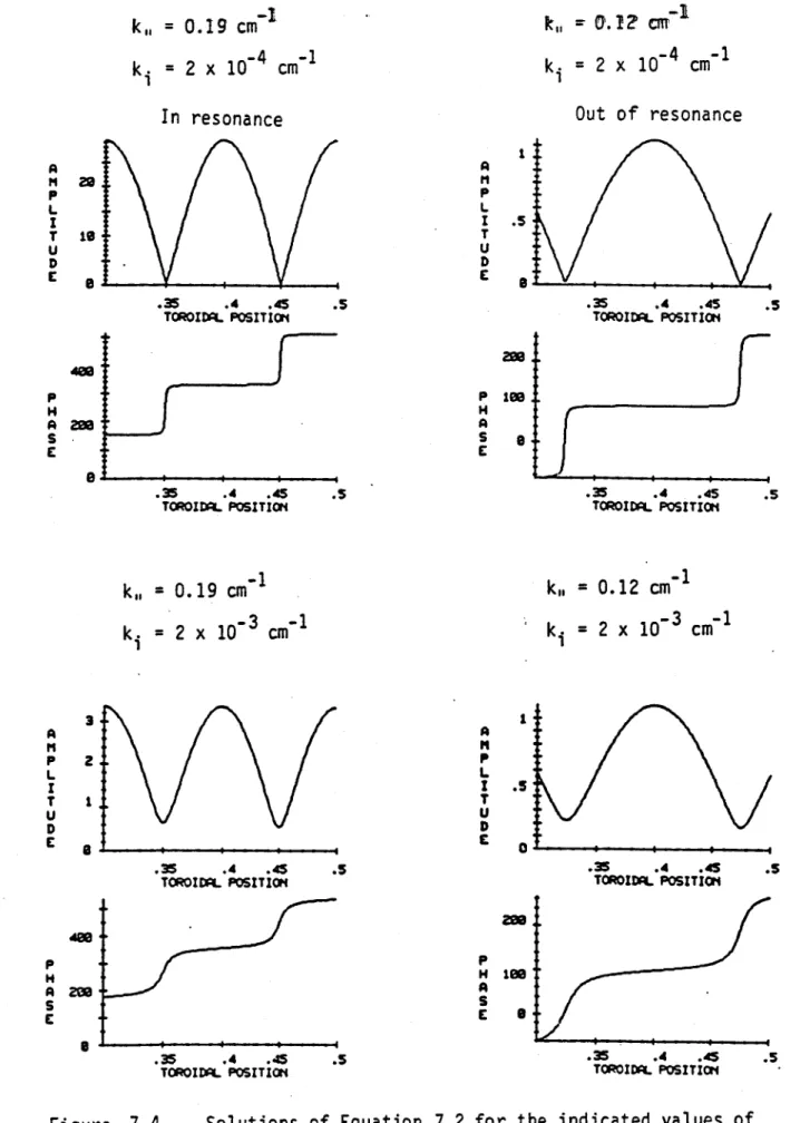
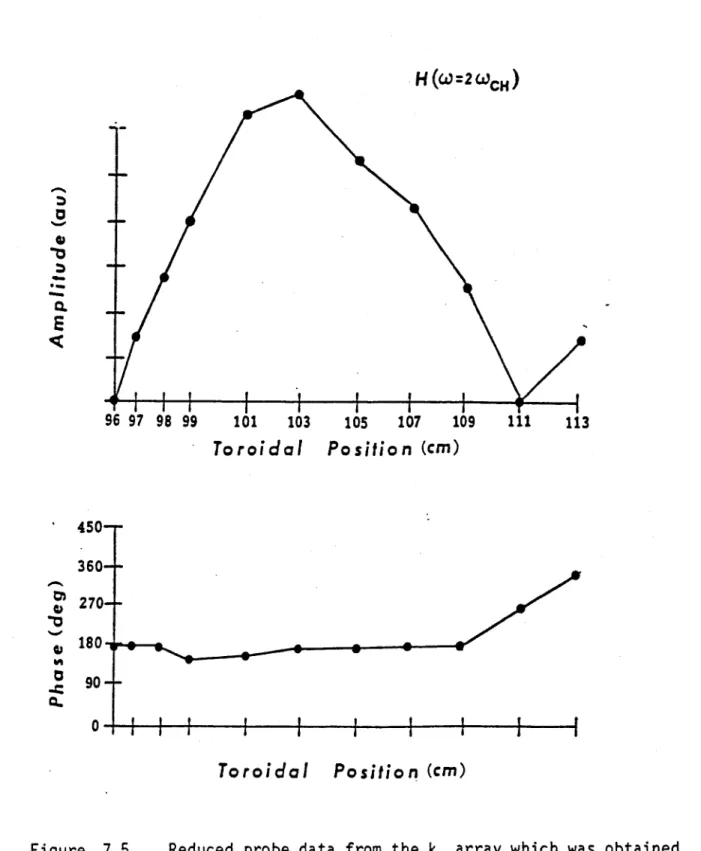
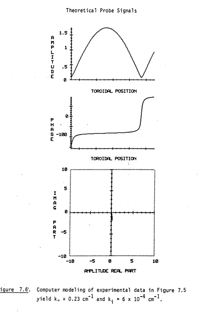
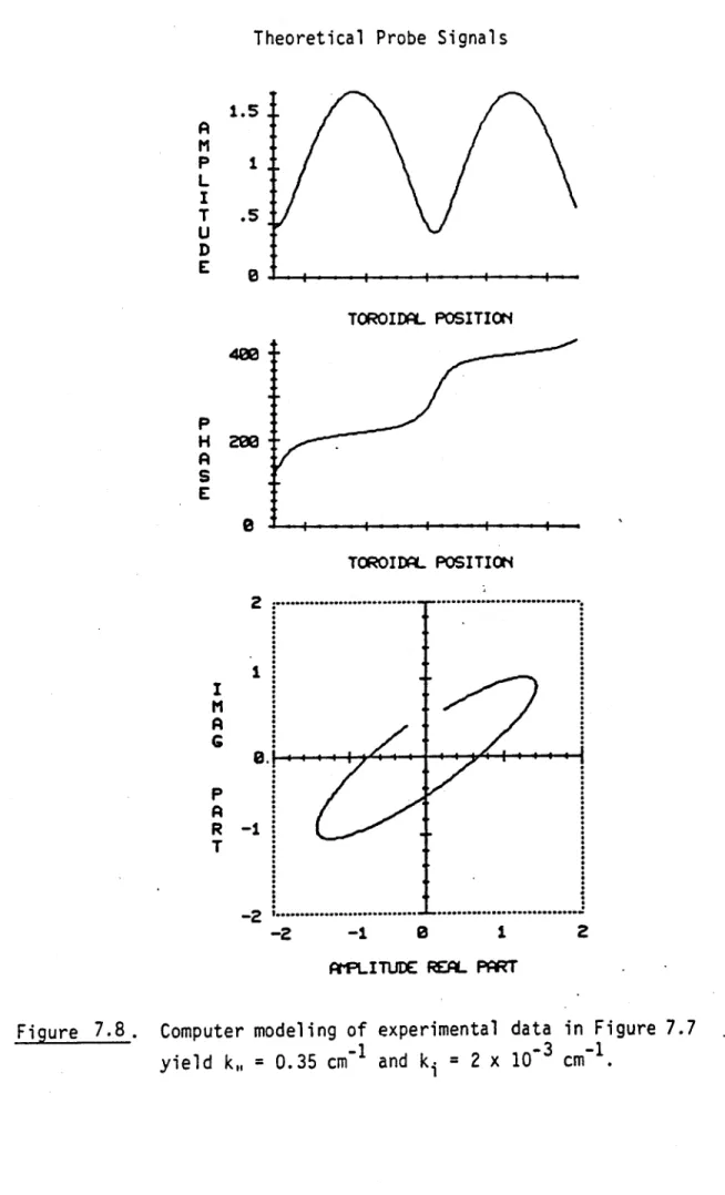
7.1. The Measurement of k, and Q... 69

7.2. Experimental Damping Mechanisms... 85

7.2.1. Deuterium and Hydrogen Minority Plasma ( w = 2_{w CD'CH}

_...

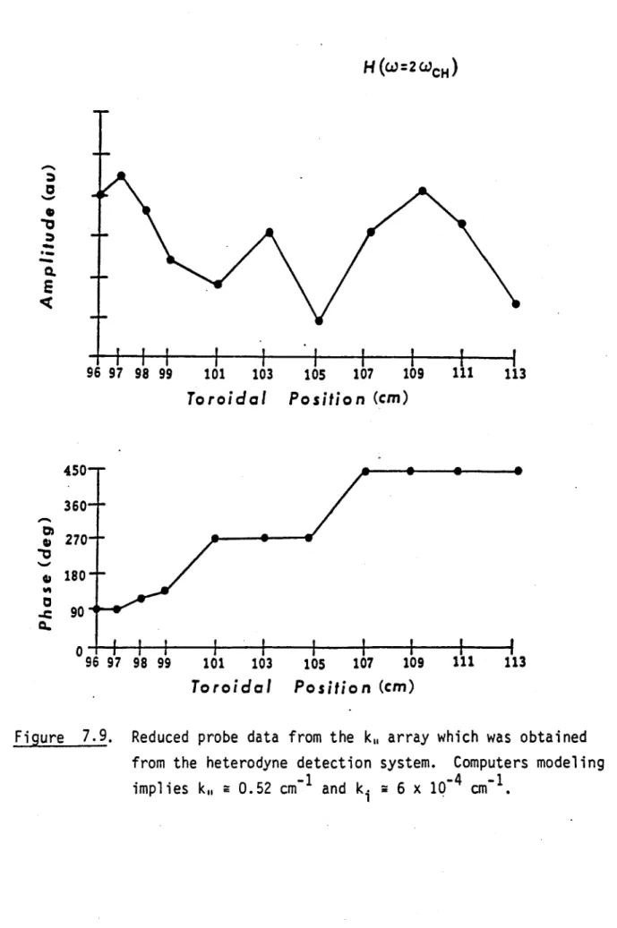
7.2.2. Hydrogen Plasma (w = 2wCH)

...---

7.2.3. Hydrogen Plasma (w - tCH

)...---

7.3. Experimental Radiation Resistance... 102

7.3.1. Hydrogen Plasma (w =wCH* -.... "... 102

7.3.2. Deuterium and Hydrogen Minority Plasma (:j = 2

wCD.'"

7.4. Parasitic Near Field Loading... 110

8. Conclusions ... ... ... ... 121

Appendix I. Mixers... ... ... 122

A.I.1. Single-Balanced Mixers. ... 122

A.I.2. Double-Balanced Mixers... 122

References... ... 129

-1. INTRODUCTION

Heating tokamaks to ignition temperature is one of the major problems arising in thermonuclear research. With present tokamak technology, the simplest and most economical method is ohmic heating. However, it becomes increasingly difficult to reach higher temperatures by this method alone because the plasma resistivity is proportional to T- 32, and the toroidal

current is limited by MHD instabilities. Neutral beam injection and RF absorption are the prime candidates for supplementary heating of tokamaks

to reactor-grade temperatures.

In the past few years, neutral beam injection has been very succesful in low density plasmas. This technique is impractical for the Alcator pro-gram because of the required beam energies for the high density regime. For this reason, plasma heating through the absorption of RF plasma waves seems to be a promising alternative. From a technological standpoint, there exists a large amount of RF power for frequencies up to a few gigaHertz, and as a result of this parameter range, several heating approaches need to be con-sidered. Different approaches can selectively heat the ions or the

electrons and modify either the bulk or the tail of the particle distri-bution function. The four major types of heating methods being explored today are:

1. Alfven-wave heating

2. Ion cyclotron harmonic heating 3. Lower hybrid wave heating

4. Electron cyclotron harmonic heating

With the unique tokamak facilities located at MIT, it is possible to examine the problems associated with heating high density plasmas. For the

past few years there has been a major effort in developing ion cyclotron harmonic heating for Alcator A, and at 200 MHz up to 100 kw of RF power has been coupled to the plasma. However, there was no noticeable change in the neutron flux rate, and the charge exchange signals had fast decay times, indicating the formation of energetic tails. In addition, the RF-enhanced charge exchange flux appeared when the cyclotron resonance was located near the plasma edge rather than in the center. Refer to Figure 1.1 for the

RF-enhanced charge exchange flux as a function of the toroidal magnetic field and position of the resonance layer.

The prime motivation of this thesis was to gain insight into the poor heating efficiencies in the Alcator A experiment by investigating the problems of coupling to fast compressional Alfven-wave. By examining wave damping mechanisms for typical parameters in conjunction with the antenna impedance a global view of the coupling process can be obtained.

n. 2.5

X

IA.U.

Figure 1.1. RF enhanced charge exchange flux vs. position of the 2_{WCH layer.}

A AI

-a

2. ELECTROMAGNETIC WAVES IN A PLASMA

Electromagnetic wave propagation in any medium is described by the general set of Maxwell's equations:

V . = / (2.1)

V x

E=

V- (0R) = ( 2.3)

vx

R

Sat

In order to utilize Maxwell's equation for wave propagation in a plasma it is useful to express the plasma current density 3 and the charge density p in terms of the local electric field

E.

n k

n£ZkckeV (2.5)

In this equation n, is the density of particles with charge eZ, and c is the sign of the charge. In order to relate V and ultimately 3 to the elec-tric field one must solve the equation of motion for a single particle. The induced motion for a particle resulting from the Lorentz force is:

m~L~

e(E

+

V

(2.6)

For the present treatment we assume that the density and background magnetic field are static in time and uniform in space. All other quantities are as-sumed to vary as exp j(k - F - t). Fourier analyzing in time and assuming

no zero-order velocities dV/dt + -j.V to first order.

-j m = ZC e(E + '. (2.7)

If the background magnetic field is in the z direction and the cold plasma approximation is used, then the solution to Equation 2.7 is (where the particle

subscript has been suppressed):

(E +j E

)(2.8)

jw

j'

With these solutions, the plasma current J can be expressed as a function of the electric field rather than of the particle velocity. The total displace-ment D and the dielectric coefficient K are defined as:

D = cOK - E =cE +

(2.11)

Equation 2.4 now takes the form v x

Fi=

jWCGK

COi( - E = K. SK K K 0 -K K 0 0 E 0 El

K,,

J

EJ

2

\w

1-~

ia--

(

-

'

K,, =

1-where k is the sum over all particle species.

In order to rewrite Equation 2.1 in terms of the electric field the continuity equation is used.

at

P =I -V

-Substituting this into Equation 2.1 and using Equation 2.11 yields:

Wave propagation in a plasma is now summarized by Equations 2.2, 2.3, 2.4 and 2.13.

The dispersion relationship for wave propagation is found by taking the curl of Equation 2.2 and substituting the result into Equation 2.4.

v x (v x T) = kO * where ko = (2.14) Defining a refractive index ni = _{lc/o and assuming ny =}

be written as: 0, Equation 2.14 can -K x K- (n2 + n 2 0

nxn,,

_Ex]

K,

- n]

Ez

J

The general dispersion relation is obtained by of equation 2.15 equal to zero. Using the quadratic for k,. the dispersion relationship becomes:

setting the determinant equation to solve

/K2 - \ kk /K \2 k+ \

kh= k2K, - ik.(+

)

-

0 where k,, = lni, and k. =- n

For a the d

two component plasma in the regime where w - wci and w 2 >> Ci

ielectric tensor elements from Equation 2.12 simplifies to: 2 k I i Wci W2() jK _L W2 K,, - .2w 2 2 where

2

Wci U.ce Lci .2 K., - nil K 2 Lnxn,, (2.16) (2.17) (2.18) (2.19)

Since

pe2>>

is reasonable to assume K,,

-.

_{Using this approximation}

and Equations 2.17 and 2.18 the dispersion relationship 2.16 simplifies to:

k ₂₍₁ -

F

)2

2)

/2

(k \

2k

/-1

)± d-

)+

y }(2.20)

A

47.n

In this equation the positive root represents the fast compressional Alfven wave or sometimes referred to as the fast magnetosonic wave. The negative root is generally evanescent in the bulk of the plasma and therefore of little interest in this class of problems.

For typical experimental conditions the following approximation is reasonable:

(1

In light of this statement, Equation 2.20 further reduces to:

k

Q

+ A

3. GUIDED ELECTROMAGNETIC WAVES

3.1 General Solution

A guided electromagnetic wave usually implies that the direction of energy flow is primarily determined by a physical boundary. This requires

an intimate connection between the fields of the wave and the currents and charges in the boundary. In comparison, the direction of energy flow for unguided waves is determined by the local group velocity of the wave and not by the physical boundaries. For most damping parameters in this experiment a wave launched by the antenna radially traverses the plasma with little absorption and is reflected off the.opposing wall. This signifies that a guided wave approach is more useful than ray tracing for determining the complete field structure in the system.

The wave guide system that we are interested in solving is illustrated below.

It consists of a cylindrical plasma enclosed by a perfectly conducting wall and a constant magnetic field in the z-direction. The plasma parameters are assumed to be independent of r, 0, and z. In the mathmatical analysis of

the problem we are required to find solutions of the wave equation which fit the boundary conditions of the wall. In the RF community it is common to

classify wave propagation into 3 basic categories.

1) TEM: _{Transverse electromagnetic waves con:ain neither electric} nor magnetic fields in the direction of propagation. 2) TM: Transverse magnetic waves contain electric fields but not

magnetic fields in the direction of propagation (Hz = 0). 3) TE: Transverse electric waves contain magnetic fields but not

electric fields in the direction of propagation (Ez = 0). Typically solutions are more complex and will contain a mixture of these modes. The best methodology in solving such a problem is to formulate Max-well's equations in terms of the field quantities Ez and H . In this way for suitable approximations the solutions break up into TEM, TM and TE modes which give physical insight to complex mode structure.

In the

previous

V X E -jWUO _(3.1)

v R = jcoK - E _(3.2)

V . (cO*( - E) = 0 (3.3)

V *

(

)

0

For the class of boundary conditions in this problem it is convenient to separate all fields into tangential and longitudinal terms. Assuming a "z"

dependence of the form exp (-Yz) and K, K _{, K, are radially independent, we} proceed as follows 2

E

ET

R

Tz z

V VT ZY (3.7)

K - E = KT

E

In the equations above a subscript T indicates that a vector lies in a plane perpendicular to the z direction. In order to facilitate problem solving later on, it is convenient to write Maxwell's equationsin terms of the field quan-tities Ez and Hz as noted before. First to find the Hz component dot-multiply iz with Equation 3.1 and substitute in Equations 3.5, 3.6 and 3.7:

iz V E = -wpoiz H

0, T Y) x(ET + z E Z) - w z - (HT + iZ)

z

VT

In a similar manner the Ez component is found by dot-multiplying iz with Eq. 3.2 and substituting in Equations 3.6, 3.7 and 3.8:

iz - x

H

jwc

E

iz T - X T + izHz wC₀ z 9 (K.ET + K iz x ET + izKtEZ)

This simplifies to:

z *.T X AT =

j

The general wave equation can be written as two second-order differential equa-tions in Hz and E . These equations are coupled through first order

substitute in Equations 3.5, 3.6, and 3.7: z X z x H zHz Note:

iz

T Ez +yT *T =T z T

Note: VT - ( x T Z vT T 2A

VT E z + Y7T T 0 z .T T Substitution of Equation 3.10 yields:

v2 E + YVT 2-kK = E

T z ~"T T = 6II E Zoo=-~ Z

2 2

where kc ₌ CO1.'O. Using Equation 3.3 along with Equations 3.5, 3.7, 3.8 and 3.9 provides an expression for the term yv T T

v -

(cO

E)

(VT z-Y) * co(KET + K i z x T +

izKE)

Note: VT i z x _{T) -z V T XT}

K vT

E

_jwOK

(3.11)

(3.12)

(3.13)

iz

Combining Equations 3.12 and 3.13 provides the first differential equation that we set out to derive:

2 'I 2

VTE

z

T

(k

The remaining differential equation is found by cross-multiplying iz with Equation 3.2 and substituting in Equations 3.6, 3.7 and 3.8:

Iz

jc1o

Dot multiply VT with Equation 3.15:

v Hz + YVT T =wcOK VT 0 z Note: VT * I _{T z xT) 'z *VT xET}T ) = T + izK,,E zI (3.15) T E - jwcoK vT

VTHz + YVT T -jw0Ka.z ' T T -

j

Substitution of Equations 3.9 and 3.13:

VT Hz + YVT T = - k2KHz - jywco K,,Ez

Combining Equations 3.4 and 3.6 expresses VT * T in terms of Hz

VT _ET

2

koK H z (3.16)

( = 0

o(V T z y) + izH z

H

-T _{= yHz} (3.17)

Substitution of Equation 3.17 into 3.16 produces the final differential equa-tion:

2

2

2

V TH z + HY+ kKa.+ k 0 : + iuwc~y -E=0 (3.18)

In order to complete the solution the tangential fields must be expressed in terms of Ez and H . It is useful to write Equations 3.11, 3.15, and iz cross-multiplied with Equations 3.11 and 3.15 in matrix form as follows:

E V TE z HV TH _(3.19) z T z XVTEz IZ z T z -Y -jwco K 0 -jwco _K, 0 -Y -jW'o 0 0 jwcoK -Y -jwc Kx -jWUO 0 0 -Y (3.20) It is possible to by M- where MM 1

solve for

E _{T E Tz} H- M1T _(3.21) z xT z xV TE z Lz xTj z x ,THzj p R Q S M = (3.22)

-Q

-S

P

R

-U

-Q

T

P

In summary, Maxwell's equations can be expressed in terms of Ez and Hz as follows:

y =

js

2

2

K

2

K,,

=0

v

_{T z}

_\$Kc/

_Kz

₊

_K

v

_(kK.

- - - WUOH = 0 (3.24)

The tangential fields are given by Equations 3.21 and 3.22.

3.2 Free-space Waveguide

This simple case demonstrates the usefulness of writing Maxwell's equation in terms of the z component of the fields. If the wave guide system contains no plasma then Kx = 0 and K, = K,, = 1. In this situation one obtains from

Equations 3.23 and 3.24 two uncoupled wave equations for Ez and Hg. The tan-gential fields are obtained from Equation 3.21.

TE Waves Ez = 0 VHz + (k - 2)H 0 T z

THZ

ET=(k,

B

)

TM Waves Hz = 0 V2Ez + (k- 2)Ez = 0 E~

V

)

s

)

For cylindrical geometry Hz ^. m(pr) for TE waves. The boundary condition at the wall implies E = 0 and Hr 0 which means dJ (pr)/dr = 0 at r = a. For TM waves Ez I- Jm(Pr) and the boundary conditions are E =, E =E 0 and Hr = 0 which means Jm(pr) = 0 at r = a. These relations determine the cutoff

wave-lengths for the TE and TM modes. The table 3 _{below shows the cutoff wavelengths}

and frequency for a cavity the size of the Alcator A vacuum vessel (a = 10 cm). Since the lowest frequency that can propagate is the TE₁1 mode at 879 MHz, one would infer that no cavity excitation will occur in the absence of plasma for the frequencies employed in this experiment.

TE Mode TE 0 1 TE 02 TE 1 TE ₁₂ TE ₂₁ TE 31 TE 41 Xc 1.64 0.89 3.41 1.18 2.06 1.49 1.18 fc (MHz) a 1,829 a 3,371 a 879 a 2,542 a 1,456 a 2,013 a 2,542 TM Mode TM 0 1 TM 0 2 TM ₁₁ TM 12 TM 2 1 TM31 TM 41 Xc 2.61 1.14 1.64 0.89 1.22 0.98 0.83 fc (MHz) a 1,149 a 2,632 a 1,829 a 3,371 a 2,459 a 3,061 a 3,614

3.3 Plasma-Filled Waveguide

If the waveguide contains a homogeneous plasma and a magnetic field in the z direction, then Field Equations 3.23 and 3.24 are coupled. The formal solution to this problem is quite tedious but fortunately reasonable approx-imations do exist. _{For the major portion of an Alcator A plasma the} approxi-mation K,-+ cis reasonable. For K,+ - and realistic values of p2 Equation

3.24 implies:

V Ez << E k K - 2

E can therefore be expressed as:

K E ' K 2W1Jo H (3.25)

(kOK.

The field equation governing wave propagation under these conditions is:

K 21 K 2 s 2_k2 V2 _{H + H k2 K. + k} 2 X 2 + A = 0 (3.26) T z Z 0 o K, k k2K, -s2

TL-The solution to this equation in cylindrical coordinates is simply of the form: Hz = HJ _{m(pr)e (3.27)} K2 K 2k2 K where p2 ₌ k2K. + k2 a2 + - + -2 o o K. k 2_K.. _$2

The remaining field quantities are derived from Equation 3.21 with EZ set to zero:

Hr P z (3.28) ___ QOj(pr)

H

li~m

J(or)\

E

r~

J

mm

m(pr

Ir

These solutions must also conform to the boundary conditions at the wall. At the wall E (r = a) = 0 and Equation 3.31 results in the following boundary

value equation:

J (pa) kK

m =-m

(3.33)

Jm(pa) pa (k OK, - a2)

This equation in conjunction with the dispersion relationship completely

discribes the wave propagation in infinite waveguide system. For = 0, Equa-tion 3.33 provides the cutoff relaEqua-tion for propagaEqua-tion:

J (pa) . K.

m() -j" . (3.34)

JM(pa) a

-For a single ion species plasma this becomes:

m (pa) M W Jm(pa)

w ci

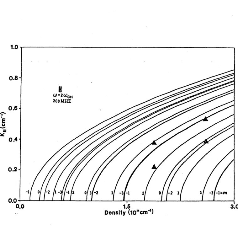
Figure 3.1 shows the solution for Equation 2.20 and 3.34 in a pure hydrogen plasma with w = 2uci when "p" is constant after mode onset. k. or a is shown as a function of density in this plot and for increasing densities higher order radial and poloidal modes can propagate.

1.5

Density (10"4cm-)

Figure 3.1. Dispersion relationship for the fast compressional Alfven wave in a hydrogen plasma with a 10 cm radius. Triangles

are experimental data points that are obtained in Chapter 7.

1.0

0.8-E

0.4

4. CALCULATION OF ANTENNA IMPEDANCE

By solving Maxwell's equations fora plasma filled waveguide we have generated a set of solutions containing a discrete spectrum of radial and poloidal modes. The problem that has to be solved now is how an aperature or loop antenna couples to the modes of the undriven system. In aperature coupling, the fields set up in the openings of a waveguide or resonant slot

are responsible for the excitation of the plasma waves. In Alcator A this scheme was not feasible because of the small port size. In loop coupling the inductive fields from currents flowing along the antenna structure pro-duce wave propagation. In this experiment loop coupling was chosen because of mechanical constraints and the excellent coupling of the loop to the fast compressional Alfven-wave.

4.1 Infinte Waveguide

In analyzing the problem for loop coupling,: it is useful to write Max-well's equations in terms of the perpendicular electric fields. We must also include a source term 3 which will represent the Fourier analyzed antenna current and ultimately excite the modes.

V XI =

-jiaIOR

v

jWCOR ' E +

3S

(4.2)

v-

Taking the curl of Equation 4.1 and substituting Equation 4.2 yields:

V

E)

Again, it is convenient to separate all quantities into longitudinal and tangential parts:

T -

8

VT X VT _{x E T} + V TXVT x iz -

j8VT

Z

_w.I

By substituting Equations 3.10 and 3.11 of the previous section, this

equa-tion simplifies to:

VT X VT x E T+ 2ET -

j$VTEZ

From Equation 4.3 we find an equation for Ez in terms of

E

V - (K -

E)

Ta

_(KT

z

)

Equation 4.5 may be written more compactly in terms of an operator L as follows:

L -

ET

WOMMOMWA06-where .

L=vT VT T T - K. - kK, 1 is the unit dyadic.

It should be noted that the homogeneous wave equation is obtained by setting

is = 0 in Equation 4.6:

L*

+

_{E =0}

(4.7)

Ti I Ti a

Equation 4.7 constitutes an eigenvalue problem of the operator L where 2Ti represents the eigenvectors and a _{i the eigenvalues of the ith mode. If ET} and J s _{can be expanded in terms of ZTi then a formal solution to Equation 4.6}

can be found. For the expansion to be valid,

E

S Re

E

E

E

The first two terms represent the individual energy of each wave while the last two terms couple the waves together. For a set of modes to be orthogonal the last terms must sum to zero which is a property of the operator L. In order to find a general procedure for determining the conditions for mode orthogonality5_,6 _{it is useful to consider the adjoint of Equation 4.7.}

-Tj + Tj = 0. L is the adjoint of L and iT= ET (4.8)

two new equations yield:

Ti -L - iTj - L -

E

If L = L then L is said to self-adjoint and has the following property:

T - L - Tdr F =

Ti

This leads to the following orthogonality relation:

S i~Tj *ETidr = 0 (4.9)

If we assume the K, infinite approximation then

L = VT x VT X

1

In this approximation L is self adjoint and the adjoint wave solution is identical 'with the original solution. This means CTi = eTj and we have an orthogonal representation necessary for expansions of the following forms:

ET

=

s = b (4.11)

where

* Edra

b. = - (4.12)

Substitution of Equations 4.10, 4.11 and 4.12 into Equation 4.6 and use of the homogeneous wave Equation 4.7 yields the following:

L *

a

'i Ti 1 Ti i Ti

ia

B + _{a 62 Ti} = -

3j4oubiCTi

I Solving for a. and substituting in b. results in:

-jwl.ob -jWJO a = - 6 8 T

_1($

Js Tidr

CTi *

Tidr,

Inverse Fourier transforming

ET

E

T(2)

ETeJB

T(Z)

=2

10

te

2

5

T

Replace $ with $j - jE and after the integraton in the complex plane has been

performed let c + 0. The poles of the integrand in complex 8-plane are shown in the following diagram.

Im(6)

IMa

0

--- Re

()

0

The path of integration leads along the real axis from -- to +- and a closed contour exists if we complete the path in the upper half plane. With the use of the residue at 6 = a we have the solution to the integral and ET becomes:

-10 s Tdr. -ji z

ET(z) = -' sTi e (4.14)

i~ - T jE r,

Once the tangential fields are known we can calculate the loading im-pedance of a simple loop antenna for the following current distribution:

js

Fourier analysis in the z directions yields:

ac _a .a

The integration of ET

-

*along the antennae is simply the back EMF induced

by the wave on the coil:

V

aCET

*

I d$

(4.16)

The terminal impedance or antenna impedance is

Z = V/It

(4.17)

Combining Equations 4.14, 4.15, 4.16 and 4.17 provides the antenna impedance

once the tangential electric fields are found:

(wO1o2$i) fd$[I($)/It Ti doi 2

Z =

LTi

t

)

$

'Ti

(4.18)

fadr

L

cTi

*

cTi

The Re(z) represents the radiation resistance while the Im(z) results from

the reactive wave field. In addition to the wave contribution to the antenna

impedance there is also an additional Re(z) due to ohmic resistive losses and I (z) due to a nonpropagating near field. These effects will be dis-cussed later on.

4.2 Toroidal Cavities

So far we have considered a waveguide system which is linear and infinite in extent. The problem of wave propagation in.a toroidal shaped device is more complicated but the methods are similar. In this geometry a wave can travel a number of times around the torus and therefore produce toroidal eigenmodes. This problem can be reduced back to a linear infinite system by using the following "image" equivalent representation.

Z=-2L Z=O Z=2L

Now the source term is composed of an infinite number of sources located at z = 2nL (n =0, 1, ±2,...)

5

Fourier transforming in the z direction yields 35 = I($)6(r - a) ~e-2 nlSL

Using the similar integration methods as before, Equation 4.18 can be re-written for the new geometry as follows:

Z = a = ( /2)

£

From Equation 3.21 and for Ez = 0, the tangential electric fields are: T + pRJ Hejm +

(.m

)

Note:

x 2 ++ 2 dx = x j 2 2 + J + 2

+ m+1x m+1 m

The antenna impedance for arbitrary poloidal mode number can be written as:

r 2 [mgJm(a C) + a r(ac fX Z. = (2arwjo) +ap (ap) 2 _{+ g2)}

_[jI

m2

g

For m = 0 and the boundary condition J₀(ap) = 0 the antenna impedance becomes:

(27mpo)[aCJ,(a _cp)/a,(a)] 2_{X i}

1 - k K (kOK, - a )

Note that for m = 0, J1(ap) = 0 and A, = 1. Important aspects of the

im-pedance equation will be discussed in conjunction with experimental results in Chapter 7.

5. DAMPING MECHANISMS

There are several different mechanisms through which RF energy can heat a fusion-grade plasma. Without careful selections of certain key parameters, RF absorption may occur at the plasma surface or at other undesirable

loca-tions. It is also necessary to understand how the power couples to the electrons, ions, minority-species ions and impurity ions in order to evaluate the

ef-ficiency of a particular heating scheme. In addition to this it is desirable to know how the energy distribution function is modified by particle-wave interaction. The waves that are excited can be absorbed by collisional and collisionfree processes by the plasma. The important collisionfree processes are cyclotron damping for the ions (fundamental and second harmonic), and for the electrons transit-time damping and Landau damping.

5.1 Ion Cyclotron Damping

Collisionless ion cyclotron damping can occur when some multiple of the particle's cyclotron frequency equals the doppler shifted wave frequency

w - k4V1 = nwci. For typical tokamak parameters this approximately occurs on a surface where n ci(R) = w. Each time an ion traverses this surface as shown in Figure 5.1, it acquires an incremental increase in perpendicular energy provided the particle has sufficient time to acquire the proper phase with respect to the electric field of the wave.

Particle absorption via collisionless processes is calculated from and E by:

Pabs= <Re(Y-E)>

This expression is dependent on the anti-Hermetian part of the dielectric tensor and is therefore zero for a cold plasma. Employing the warm plasma dispersion relation and suitable approximations Stix 7 has shown that the

Circulating Particles

Particle Orbit

Figure 5.1.

x

Cyclotron Resonance Layer

Trapped Particles

Wave Field

W ci

h7

An ion is continuously accelerated by wave field when w = wci' However for w = 2 wci there must be a gradient in the electric field or the toroidal magnetic field in order for ions to gain net energy.

V

I

average power absorbed per unit volume by the ions is:

2 n-l 2

C -c i k!V,2 - n wc i E2

P/unit volume = 2kV 2)f ekxpV _|ELI

where n = ion cyclotron number and

2kT 1/2

T _mi

Since wci is proportional to l/R, the exponential function is appreciable only over small distances on the order of:

2k.,VtR ex =

nwCi

2

Assuming that IELI ' wpi, k,,, and VT are constant over the resonant zone 6x, then the following integral represents the total average power absorbed:

T= x 2 R (unit ol dr

where "R" is the major radius and "a" the minor radius.

For concepts dealt with in this thesis, the dimensionless figure of merit Q is or more use than the specific formula for power asorption. For second harmonic resonant heating Paoloni 8 has derived the following

2 22k 2 + k+1+ Q2c 2 (5.1) 2 k 2V2 where: = 1/2 (kr)2 2 T 2w ci Vp = W (k2 + k ) 1 _{2- -_, 2)} k,1T k A- ki

This procedure is also valid for plasmas containing a minority ion species. In this case the properties of the fast wave (wave energy and

EL) are approximately determined by the majority component and the minority only effects the power absorption. When the minority fundamental reson-ance layer is in the center of the plasma, Paoloni expresses the Q as:

2 2

A kA)

MIN 2 ( + )2 (5.2)

where wp and w ci are evaluated for the minority component in

It is also important to know whether the power is deposited in the bulk or the tail of the ion distribution. For typical tokamak parameters,

coulomb collisions during poloidal circumnavigation times will cause random phase delays among particles leaving the resonant zone. This implies that each transit through the resonant zone is independent of past history with respect to phase. Once this is justified it is valid to derive a Fokker-Planck equation which will govern the quasilinear evolution of the ion velo-city distribution. This is essential since most quasilinear calculations de-mand randomly-phased modes to justify the concept of true particle diffusion resulting from a number of incoherent velocity displacements. Although this thesis deals primarily with the concepts of absorption mechanisms, it is important to grasp this major point in the evolution of the distribution function.

5.2 Ion-lon Hybrid Resonance Damping

Energy of the fast magnetosonic wave can also be absorbed via the ion-ion hybrid resonance provided a minority ion-ion species is present. The dispersion-ion relationship for the K,, - approximation can be factorized in the following form:

(K - n2) = (n - R) -

L)

The ion-ion hybrid resonance will occur at the surface where K, - n, = 0 which implies n, + C. In reality n, # -and a sequence of mode conversions will result.

This class of problems has a closely spaced resonance and cut-off layer which is approximately described by Budden's equation. Perkins 9 and Swanson 10 have obtained absorption, reflection and tunneling coefficients for this process. When deuterium is the majority component and hydrogen is the

minority component, the hybrid layer is located on. the high field side of the fundamental layer. On the major axis, the approximate position is given by:

[

r+A

N12

r

Z A

N

RION-ION = R 1 +

J

1 1 1Z2A22

R is the major radius, A., Z., N. for i = 1,2 are respectively the mass num-ber, the charge numnum-ber, and the density (i = 2 is the minority

compon-ent). This layer is sensitive to the relative concentration of species and, for 95% deuterium and 5% hydrogen, it lies about 1.8 cm from the cyclotron resonance.

Since kit for the fast wave is very large near the resonance layer, the mode-converted wave must have a comparable kit for good coupling efficiency. The converted wave is believed to be a class of Ion Bernstein waves. Because this wave propagates away from the narrow hybrid layer and it has a relatively large kit, electron Landau damping is important. For small proton

concentra-tion the hybrid layer lies close enough to the cyclotron layer implying that the Ion Bernstein wave can also undergo cyclotron damping before the wave is completely Landau damped. This means that both ion and electron heating could occur for this process. Perkins computes the damping for this process as:

IT p/p 2Z 2 P)(ucD - wH)

Im(k) = 4R 2kit ( 2(5.4)

wheisthe prc2tnCD ttn -cn

Since it is possible for the ion-ion hybrid layer to lie close to the cyclotron layer, their effects cannot always be separated in a practical experiment. It should be noted that the presence of the ion-ion hybrid resonance also effects the absorption at the ion cyclotron layer. The hy-brid layer alters the wave field polarization in the vicinity of the cyclo-tron layer by increasing the left-hand component of the field. This en-hances the cyclotron absorption, but this effect becomes insignificant for densities above 0.35 x 1014 cm-3,

5.3 Electron Landau and Transit-Time Damping

Electrons can absorb a considerable amount of energy from the wave when the phase velocity is near the electron thermal speed. Particles for which

S- kV e = 0 undergo Landau damping and transit-time magnetic pumping. In transit-time damping the wave acts on the particle through the force - WB and for Landau damping the particle force is qE. These mechanisms are re-lated through the phase of 9 and E, and therefore not independent. Stix

has shown that the average power absorbed per unit volume by the electrons to be:

V p 2 (V /V )2' 2

P/unit volume = e 2e 2e V)2T(

Integrating the equation over the plasma volume and using the total wave energy Paoloni 8 has determined the Q to be:

1 /c)e2e 2 [ 12 2~+l'

C(_ V(Vp/VTe 2 I k 2 +k + I + 1 (5.5)

5.4 Ohmic Collisional Damping

In low temperature plasmas ohmic collisions can absorb power from the wave. The average power lost per unit volume for collisions is:

P/unit volume = R (-E) = 1 R [(a-E) -E]

2 e 2 e

For the fast wave, Paoloni8 _{has found the}

_Q

Q

col

n.

where ri = 0.5 x 10'4 lnA/T _{. e} 3/2(T in eV). _e When the temperature is above 10 eV, collisional effects are unimportant compared to other damping mechan-isms. Basically, the high conductivity of the plasma forces Ez to be extremely small, preventing energy transfer through collisions. Despite the low tempe-ratures at the plasma edge, collisional effects still remain insignificant because for typical density profiles Ez is still small in the edge region. 5.5 Wall Loading

Since we are dealing with guided waves, some power will be lost in the finite conductivity of the vacuum chamber walls. Jackson1_{2 uses a simple}

approximation method in order to solve this problem. Using the fields ob-tained from the ideal boundary conditions, one finds the fields within the conductor by using Maxwell's equations. Ignoring the displacement. current, the electric field in the conductor is:

This small tangential component of T in association with the tangential com-ponent of W implies that there is a net power flow into the conductor:

P/unit area = Re (E x H- r =a Paoloni 8 calculates the value of Q for wall loading as:

Z

= A 2 + k + 1)2 + 1 e2k 6

where s (f) -1/2

6 = distance between plasma and wall = 2nR

ks = surface length of the torus

For the Alcator A experiment tT As % 0.5. This geometrical factor is based upon wall corrigation and port size.

5.6 Fundamental Single Species Ion Cyclotron Damping

It turns out that heating ions via the fundamental cyclotron resonance in a single species plasma is a poor choice. Despite the strong coupling between the electric field and the ions, the left-hand component of the elec-tric field is quite small because it is shorted out by the large number of

resonant ions. The overall absorption is weak and Perkins 9 estimates the Q to be:

Q

(

In competition with fundamental cyclotron absorption layer is the ion-cyclotron mode conversion layer near the surface of the plasma. As stated previously, the dispersion relation can be expressed as:

2 2 2 _{_R)(2 _L}

n(k.,) = (n - R)(n - L)

Mode-conversion will occur at the surface where k., - n 2 = 0. For n = 1.5 x 1014 and typical experimental parameters at 90 MHz, this surface is about 1 cm

from the plasma edge. The conversion occurs on the high field side of the fundamental layer. Perkins 9 develops a simple slab mode and dispersion re-lationship for estimating the effects of ion-cyclotron mode coversion. The estimated Q for the process is:

2 2

RIC (5.9)

For Alcator A parameters the power absorbed by this process is larger than fundamental absorbtion. This means the wave can easily tunnel through the center of the machine and be absorbed near the plasma edge when launched from the low field side. It should also be noted that ion-cyclotron mode conversion doesn't occur for second harmonic heating experiments in a single species

2 plasma since k~ . 0.

6. EXPERIMENTAL APPARATUS

The equipment used in this experiment falls into two distinct groups. The first group deals with wave generation and consists of the transmitter

chain, matching network andthe antenna structure. The second group uses RF diagnostics to analyze wave propagation and covers the measurement of radia-ti.on resistance, probe signals and k,,.

6.1 Antenna System

Designing an antenna structure for Alcator A isa very difficult task be-cause of the compact nature of the machine. The vacuum ports in Alcator A are very small as a result of the Bitter magnet design, large compressional forces on the flange,.andthe need for small ripple in the toroidal magnetic field. The largest single hole is 1.25" by 3.4" which introduces stringent mechanical constraints on the antenna design. It was necessary to develop an antenna which could be slid in horizontally and then rotated vertically. With the aid of various insertion jigs, an antenna which subtended a poloidal angle of 130* could be installed on the low-field side of the torus. In the course of this

13

experiment, three different antennae were develoned. All three antennae were center fed one-half turn magnetic loops as shown in Figure 6.1. The first an-tenna (A1) was machined out of a solid block of 304 stainless steel. Structural

integrity was a main issue in this design because of the proximity of the plasma and the antenna. The sides of this steel block were slotted, and narrow clips were E-beam welded across the front face, which resulted in a simple faraday shield. The purpose of the faraday shield was to short out the EZ component of the near field and prevent coupling to undesirable parasitic modes. The fara-day shield also reduced the plasma density near the center conductor. At each

end of all three antennae, small probes were used to monitor RF antenna cur-rents for radiation resistance measurements. These probes were inserted through vertical access ports after the antenna was installed.

The A₁ antenna was finally abandoned because of insufficient radiation resistance which resulted from a poorly designed faraday shield. The A₂

antenna had about three times more radiation resistance than the A, configura-tion, and therefore more power could be coupled to the plasma. The antenna had a loop area two and a half times larger than the previous design, which increased the radiation resistance significantly. The loop area was increased by reducing the plasma radius from 10 cm to 9 cm enabling the distance between the wall and the center conductor'to be increased. It also had a wider center conductor which lowered the antenna terminal impedance and helped prevent arcing. In favor of higher radiation resistance, it was decided that a faraday shield would not be incorporated in the deisgn. However, in order to reduce the plasma density in the vicinity of the antenna, two slotted limits were positioned adjacent to the antenna. Figure 6.2 shows the orien-tation of the limits with respect to the antenna. Although this antenna coupled more power to the plasma, there was no strong evidence of plasma heating, alluding to the fact that parasitics were indeed a problem. The third and final antenna tested was A4. Basically, we removed the faraday

clips on A₁ and moved the center conductor three times farther out. New curved faraday clips were welded on and the side limiters from the A2

con-figuration were also installed. With these modifications the A4 antenna

had twice the radiation resistance of the A1 antenna. See Figure 6.3 for

a picture of the design. Although it is not visible in any of the photographs, the center conductors and the inside surfaces of the black planes of all

three antennae were silver-plated by standard electroplating techniques in

SOMINOMMOMMOWN-Virtual Limiter r = 12.5 cm r = 10 cm r= 9. 5 cm Figure 6.1. 10 cm 0 .187 0.542"0 RF Probe jS 0. 625"

Front and side sectional views of the three antenna configurations tested in Alcator A. Only A₁ and A₄ were equipped with a

faraday shield. Note RF probe used to monitor antenna current for radiation resistance measurement.

pI

I

-1

r-~

E.~.

~1

LL-'IALI 0 .4-J 41 -I-

j'4

6.2 Matching Network

In order to ensure low VSWR on the transmission line between the transmitter and antenna, a matching network was constructed. The matching system was

designed for a 1 _{MW experiment and as a result it is quite large.} Figure 6.4 shows the 9" coaxial transmission line which couples the matching cavity to the transmitter chain. The cavity length and tap angle of the 9" input coax are tunable in order to match the antenna impedance to the 500 transmission line. At 200 MHz the cavity is tuned to one and one half wavelengths and for 90 MHZ

operation, set to three-quarter wavelengths with the lower shorting plate removed. The resonator is connected to the antenna by means of two 1" vacuum coaxial lines. Due to the poor conductance between the Alcator A vacuum vessel and the coaxial lines a 30 liter/sec high-Q ion pump was installed which maintained low pressure in these lines. Figure 6.5 shows a detailed view of the antenna and coaxial feeders. All these components are connected directly to the tokamak and voltage isolation from the resonator to the coax center conductors is provided inherently by the magnetic coupling loop. On the other hand the outer conductor of the coax feeders are connected to the resonator through a teflon by-pass capacitor. In this way there exist complete DC isolation between the tokamak and all RF components except for the coaxial feeder assembly. The antenna and 1" _{coax feeders are made from 304 stainless steel that was silver plated} 0.001" to reduce resistive losses. All the RF current flows in the silver plating since at 200 MHz the skin depth is 2 x 104 inches. Most of the

system loss occurs in the two coaxial feeders, and the resistance is calculated from the following equation:

R =(6.1)

where, for silver, o = 6.1 x 10 mho/meter, k = 1 meter/line, and 6 =(2/W900)1.

The theoretical resistance of both coaxial feeders at 200 MHz is R = .32, while the measured resistance for the system was R = 0.5*.

Resonator 00, 01 Ilooo 11011 1-00: 9" input line

E&IZI

i

Location of the coaxial resonator with respect to Alcator A. This system was used to match the antenna impednace to 50R

transmission line. In order to tune the system a servo

mechanism was used to adjust the position of the upper plate, lower plate and tap angle.

Resonator

Coaxial Feeder Assembly

ion PUMP

light .bitter

detector light detector

flange-and window

ceram c _{ion pump}

mylar DC block

Figure 6.5 . Detailed view of the coaxial vacuum lines used to drive the antenna. Ion pumps were used to maintain high vacuum in the lines as a result of the poor conductance to the main vacuum chamber. Note the ceramic RF vacuum breaks located inside

6.3 Transmitter System

A 1,000-watt broadband amplifier was used for all measurements of antenna resistance and k.. The versatility of this amplifier enabled us to change the freauency from 90 MHz to 200 MHz without tuning the transmitter. The trans-mitter is based upon a distributed amplifier configuration and has 10 Eimac tubes which are senarated by an equal number of electrical degrees. The arid line and plate line are ecuivalent to a terminated lumped-element transmission line where the electrode capacitance and external inductors are the key elements. When an RF signal is applied to the grid input, a wave travels along the

grid line, and the various tubes are gated into sequential conduction. For any tube gated into conduction, one half of the plate current travels toward the load end of the plate line while the other half travels toward a termina-tion resistor. Because of the phase tracking in the plate and grid lines, the phasor sum of the individual tube currents add and the signal is amplified by a factor of 0.5 N (N being the total number of tubes). The broadband nature results from the fact that the plate and grid circuits behave like terminated transmission lines and therefore the impedance is independent of frequency. This configuration also has the advantage that the power output is constant even with poorly matched loads.

For the high-power heating experiments on Alcator A, the 1 KW amplifier was used as an excitor for a 100 KW pulsed Class C amplifier. The Class C amplifier used an RCA 2041 tetrode in a half-wavelength transmission line cavity. This tetrode in turn drives a grid pulsed RCA 6550 triode and can be tuned from 170 MHz to 220 MHz. The 6950 is a double-ended coaxial

super-power, shielded-grid beam triode mounted in a 30n0 coaxial cavity and delivers 1 MW. Through suitable RF switch gear it was easy to switch from 1 KW to 1 MW.

6.4 RF Probes

In order to study key features associated with the propagation of the farst compressional Alfven wave, a number of RF probes were positioned near the plasma edge. Specifically the probes were located near the antenna,

one-quarter and half way around the torus. Although these probes were located in the evanescent fields associated with the vacuum layer, a great deal of information can still be obtained. The typical probe consisted of a one-turn magnetic .loop connected directly to a coax cable. All RF diagnostics used double-shielded RG55 coax in order to minimize Dickup and, for typical lengths of 50 ft., the losses were 3.5 dB at 200 MHz. A Tektronix 7834 storage main-frame was used for acquisition of the probe data. The 7834 oscilloscope has a

stored writing speed of 2,500 cm/Vs, enabling one to display single-trace rise times of 1.4ns. The pre-amp used with the mainframe was a 7A24 which is a high-performance, wide-band, dual-trace amplifier from DC to 400 MHz with 5 MV sen-sitivity. Both inputs are 500 terminated with a VSWR of 1.25:1. With the 7834

and two 7A24 plug-ins, four RF traces could be stored at a time.

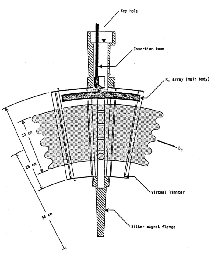
6.5 K, Array

An important parameter in this experiment is the value of k,, since mag-netude of wave damping and even the type of damping are strongly affected by it. In order to measure k, we developed an eleven-probe array which monitors the phase and amplitude of the wave in the toroidal direction.