HAL Id: inria-00554738
https://hal.inria.fr/inria-00554738
Submitted on 11 Jan 2011
HAL is a multi-disciplinary open access
archive for the deposit and dissemination of
sci-entific research documents, whether they are
pub-lished or not. The documents may come from
teaching and research institutions in France or
abroad, or from public or private research centers.
L’archive ouverte pluridisciplinaire HAL, est
destinée au dépôt et à la diffusion de documents
scientifiques de niveau recherche, publiés ou non,
émanant des établissements d’enseignement et de
recherche français ou étrangers, des laboratoires
publics ou privés.
Spatial Complexity of Reversibly Computable DAG
Mouad Bahi, Christine Eisenbeis
To cite this version:
Mouad Bahi, Christine Eisenbeis. Spatial Complexity of Reversibly Computable DAG. international
conference on Compilers, architecture, and synthesis for embedded systems, Oct 2009, Grenoble,
France. �inria-00554738�
Spatial Complexity of Reversibly Computable DAG
Mouad Bahi
INRIA Saclay - Île-de-France and LRI, Université Paris-Sud 11
Orsay, France
[email protected]
Christine Eisenbeis
INRIA Saclay - Île-de-France and LRI, Université Paris-Sud 11
Orsay, France
[email protected]
ABSTRACT
In this paper we address the issue of making a program reversible in terms of spatial complexity. Spatial complex-ity is the amount of memory/register locations required for performing the computation in both forward and backward directions. Spatial complexity has important relationship with the intrinsics power consumption required at run time; this was our primary motivation. But it has also impor-tant relationship with the trade off between storing or re-computing reused intermediate values, also known as the rematerialization problem in the context of compiler regis-ter allocation, or the checkpointing issue in the general case. We present a lower bound of the spatial complexity of a DAG (directed acyclic graph) with reversible operations, as well as a heuristic aimed at finding the minimum number of registers required for a forward and backward execution of a DAG . We define energetic garbage as the additional number of registers needed for the reversible computation with re-spect to the original computation. We have run experiments that suggest that the garbage size is never more than 50% of the DAG size for DAGs with unary/binary operations.
Categories and Subject Descriptors
D.3.4 [Programming languages]: Processors—Compil-ers; F.1.2 [Computation by abstract devices]: Modes of computation—Parallelism and concurrency
General Terms
Design, Theory
Keywords
Reversible computing, Spatial complexity, garbage minimiza-tion
1.
INTRODUCTION
One of the most important barriers to the performances of processors is power consumption and heat dissipation. Sev-eral works consider how to make architectures and programs
Permission to make digital or hard copies of all or part of this work for personal or classroom use is granted without fee provided that copies are not made or distributed for profit or commercial advantage and that copies bear this notice and the full citation on the first page. To copy otherwise, to republish, to post on servers or to redistribute to lists, requires prior specific permission and/or a fee.
cheaper in terms of energy. Thermal models are designed based on underlying electronics for architectures, or based on some software rules for programs, for instance balancing resources usage [23], or minimizing caches misses, or cutting unused devices. There is also a radically different approach that tackles energy issues under the point of view of intrin-sics thermodynamics of computation and the basis argument that likewise thermodynamics transformations, irreversible programs have to dissipate heat. This originates from the Landauer remark [17] that erasing or throwing away a bit in-formation must dissipate at least kT ln2 of energy. Therefore only reversible programs are likely to be thermodynamically adiabatic. Reversibility means here that no information is ever lost, it can always be retrieved from any point of the program.
Reversibility of programs has then been studied by Ben-nett [2]. A first easy way to make a program reversible is to record the history of intermediate variables along the execution, but then the issue of erasing - forgetting - that information, called garbage, remains. That garbage can be used as an estimation of the intrinsics energy consumption of programs and minimizing it is the objective. Bennett[2] proved that if the input can be computed from the output then there is a reversible way of computing the output from the input while eliminating the garbage. This may be at the price of large space usage for storing all the intermedi-ate stintermedi-ates during the computation. The alternative is to use checkpoints where the state of computation is stored and therefore from which the computation can be restarted for computing subsequent results. This is the very classical is-sue of trade-off between date storage and data recomputing in several domains of computer science.
It should be noted that evaluating energy with the size of garbage is not natural as one would better tend to relate energy with time complexity. Matherat et al. [20] elabo-rate on this point. They suggest first that convergences in state automata are the major sources of information loss and therefore heat dissipation. Second in the same idea as convergences they insist on the role of synchronisations in heat dissipation.
Reversibility of computation has several applications, among which we can mention bidirectional debuggers [8, 15], roll-back mechanisms for speculative executions in parallel and distributed systems, simulation and error detection tech-niques [6]. There are also algorithms that require a pass CASES’09,October 11–16, 2009, Grenoble, France.
where intermediate results have to be scanned in reverse or-der. This happen for instance in reservoir simulation, or for instance in automatic program differentiation [12]. More-over reversible processor architectures have already been designed [14, 10], as well as reversible programming lan-gauges [10, 18].
In this paper we analyze the reversibility of computations with two aims. First we want to characterize the intrinsic reversibility of a program or piece of program based on its data dependency graph and not on some linear sequence of instructions. We hope this helps us understanding where energy bottlenecks arise from in ordinary programs. Sec-ond, because reversibility is very close to the trade-off be-tween data storage and data recomputation, we want to ana-lyze whether reversing operations or a set of operations may make the compiler problem of data rematerialization easier. An important hypothesis in this paper is that the opera-tions that we consider can be reversed, this may concretely cause several problems that we skim over. We consider only DAGs (directed acyclic graphs), this means basic blocks in DDG (data dependency graphs). Compared to other works we consider possible rescheduling of instructions instead of a fixed sequence of already scheduled instructions. And the question that we address is: ”Given a DAG computation graph with reversible operations, what is the minimum amount of garbage necessary to make the whole DAG re-versible?”
Our ambition is therefore modest compared to this major and important issue of understanding precisely the relation-ship between physics, information, measurement, observers in one hand and information theory, computing in the other hand [11]. We believe however that this work may help op-timizing scheduling and data storage in applications men-tioned just before.
The remaining part of the paper is organized as follows. In Section 2 we explain more precisely our basic hypothesis and how we relate the problem of garbage minimization to the problem of register allocation, namely the number of regis-ters required for reversibly executing the computation DAG. We give a heuristic algorithm for finding the number of addi-tional registers (“garbage”) required. In section 3 and 4, we propose a lower bound based on the decomposition of DAG into elementary paths and we compare the values lifetime between reversible and irreversible computing. Systematic experiments (section 5) with our heuristic algorithm sug-gests that garbage is never more than n/2 where n is the operation count in the DAG. We conclude (section 6) by a discussion on related works as well as our future work on storage and data recomputing for the minimization of mem-ory access.
2.
COST OF REVERSIBILITY
AND ALGORITHM
In this section, we present our approach and algorithm for computing the spatial complexity of reversing a DAG. We consider a DAG of operations, typically the Data Depen-dency Graph of instructions within a basic block, see the part (a) of figure 1. Nodes of the graph are instructions de-noted by the name of the variable carrying the result. This makes sense as two different nodes need to be treated as
two different variables. We consider only unary and binary operations and we make the important hypothesis that they can be made reversible.
2.1
Reversible Operations
A boolean function f (x1, x2, ..., xn) with n input boolean
variables and k output boolean variables is called reversible if it is bijective. This means that the number of outputs is equal to the number of inputs and each input pattern maps to a unique output pattern. Based on that we make the very rough abstract approximation that the operations in the DAG are reversible in the following sense: for unary op-erations, they are bijective so that the operand is uniquely determined by the result. For example, consider the incre-ment function, defined from the set of integers Z to Z, that to each integer x associates the integer y := x + 1. The inverse function is x := y − 1, easly determined from the result uniquely. For binary operations, this means that only one additional value beside the result is needed for recover-ing both operands from this result and this additional value. This is typically the case of the basic arithmetic operations, like addition c := a + b, where (a, b) can be retrieved from (a, c) or (b, c) by a simple subtraction. Hence the ’+’ oper-ation is considered as having two operands and two results. This is only an abstraction and we are aware of a number of flaws underlying the concretization of this assumption. For instance the multiply0∗0operation needs at least one addi-tional resulting bit for determining which of both operands was 0 if the result is 0. There are also data precision is-sues especially with floating point operations and round-off problems but we neglect them and count only the number of data as a measure of memory/register space. We could also consider the semantics of operations and transform the operations in order to minimize the space for storing inter-mediate results. This is for instance done by Burckel et al. in [7] where they show that the computation transforming n inputs into n outputs can be (reversibly) performed by us-ing a storage space not greater than n. Therefore in our ab-stracted model, when executing a binary operation we have the choice of memorizing the first or the second operand or both, provided that the reverse operation is possible based on the result and memorized operands.
What we want to evaluate is the maximum size of storage needed to execute the operations of the DAG reversibly in a forward and backward execution, or in other words we want to minimize the history required for performing the DAG reversibly. The additional storage space required compared to a simple forward execution is our criterion of “energetic garbage”. With this criterion we want to characterize the intrinsic energetic cost of the DAG. Compared to the Ben-nett strategy for minimizing the storage space with check-points we have the degree of freedom to choose the ule of operations. Finally our problem is finding a sched-ule that minimizes the register requirement in a forward and backward execution. The difference between the bidirectional execution and the forward execution is called the energetic garbage.
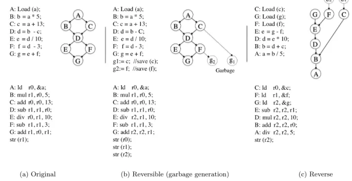
As an illustration, consider the code segment shown in fig-ure 1(a) with its corresponding pseudo-assembly code and dependence graph in which each node corresponds to a
state-(a) Original (b) Reversible (garbage generation) (c) Reverse Figure 1: Illustrative example of reversible code and garbage generation.
ment in the code segment. This pseudo code requires only two registers. Figure 1(b) shows a reversible code that re-turns the same result as the code in the figure 1(a) and saves also two intermediate values. This code requires three reg-isters for the three outputs g, f and c. Figure 1(c) shows the reverse code and its corresponding reverse graph derived from the reversible code in figure 1(b). It shows how a re-verse computation could be perfomed to generate all pre-vious values. Thus, 2 registers are required in the forward computation, 3 in the forward and backward computation. The energetic garbage is 1.
2.2
Algorithm
Like all optimization problems in register allocation it is likely that garbage minimization is a NP-complete problem. But we have not proven it. Here we describe a heuristic that schedules a DAG in the direct order while keeping some variables alive in order to make the backward computation feasible. We call garbage the difference between number of registers in the direct computation and number of registers in the schedule found in this algorithm.
Starting from the input data, the DAG is scheduled first in the direct direction and then in the reverse direction and we are looking for a schedule that uses the minimum number of registers. Since we consider a DAG, the number of regis-ters required by a schedule is also the maximum number of simultaneously alive values during direct and reverse com-putation. One of the main issues of this work comes from the need to deal at the same time with the constraint of the minimum number of registers and with the constraint of saving values for enabling backward scheduling (reversibil-ity constraint). Our algorithm decides two kind of informa-tions: first which intermediate values will be saved in order to make the reverse computing feasible and second which successor node will kill the value - and hence will reuse the
same register in the actual register assignment of the direct computation.
The algorithm scans the DAG G = (V, E) and schedules instructions in some topological order only in the direct di-rection. V is the set of nodes and E the set of edges. At each step the instruction with highest priority is selected. Algorithm is presented on the following chart.
Input: DAG computation graph.
Output: number of registers required for reversible com-puting
Figure 2: Scheduling algorithm diagram. a. Priority
1. The order in which ready instructions are selected affects the number of registers required and the garbage size. 2. We use a heuristic.
3. Our scheduling is based on minimizing the number of resources (registers) without time constraint.
4. We favor instructions that have more predecessors with a minimum of successors in the DAG (this allows to use less registers)
5. We favor instructions on the critical path. This will in-crease the number of calls to the scheduler.
We reuse only registers of the direct predecessors (to pre-serve information).
b. Labeling
Each node can take one of the following labels:
Active: if the value of a node is already computed and avail-able in one of the registers.
Passive: any already calculated node that will not be used in a future computing.
Ready: if the value of a variable is ready to be calculated and all its predecessors are actives.
Idle: a node that is waiting because one of its predecessors is still waiting (waiting for all its predecessors to become ac-tive). Initially all source nodes (nodes without predecessors) are set to Active, the others are set to Idle.
Labeling rules
Let us consider the functions λ and Ω that define the state of a node u from the set of global nodes V
λ : V −→ {Active, P assive, Ready, Idle} u −→ λ(u)
Ω : V −→ {Selected, N ot selected} u −→ Ω(u)
These rules are applied at each stage of calculation. Γ+G(u) (resp. Γ−G(u)) is the set of successor (resp. pre-decessor) nodes of node u.
∀u ∈ V ∧ |Γ−G(u)| = 0 ⇒ λ(u) = active ∀v ∈ Γ−
G(u) ∧ λ(v) = active ⇒ λ(u) = ready ∃u λ(u) = ready ∧ Ω(u) = selected ⇒ λ(u) = active Stop condition
∀u ∈ V : λ(u) = active ∨ λ(u) = passive
The final number of active nodes is the number of registers required.
The active nodes represent also the footprint needed for re-versing the DAG computation.
Selection Algorithm
As an entry, the list of values ready to be calculated Rule 1: u is the unique successor of v that remains to be scheduled: u will reuse the register used by v.
if ∃u ∈ V λ(u) = ready {
if ∃v ∈ Γ−G(u)/|Γ+G(v)| = 1 { Ω(u) = selected; λ(v) = passive; } else if ∃v ∈ Γ−G(u)/∀w ∈ Γ+G(v) ∧ w 6= u ∧ λ(w) = active { Ω(u) = selected; λ(v) = passive; }}
Rule 2: Among ready nodes, one node with most successors is selected. For each pair of ready nodes u,v ∈ V
∃u ∀v (u, v) ∈ V λ(u) = λ(v) = ready if |Γ+G(u)| ≥ |Γ+G(v)|
Ω(u) = selected;
The second rule is applied if the first rule fails to select an instruction (node). Once we find the selected instruction, we go the labeling rules.
c. Guarantees
This algorithm ensures that all nodes will be covered, in
Nodes A B C D E F G H I J K L M N O P Initialization A I I I I I I I I I I I I I I I Labeling A R R I I I I I I I I I I I I I Selection - - S - - - -... Labeling P P P P A P A P P P A P A A A R Selection - - - S Labeling P P P P A P A P P P A P A P A A A: Active P: Passive R: Ready I: Idle S: Selected
Table 1: An execution of the algorithm described by relabeling and selecting rules (corresponding to the code of example 2 figure 3)
other words, all values will be calculated. At the end active nodes contain active registers that will be used in the back-ward generation of all values.
d. Analysis
We can show that the following algorithm allows selecting a high priority instruction, which consumes less resources, at least at each computation step, this is a local optimization. At each computation step only one instruction is selected. The first rule allows the node who has a predecessor with one successor or predecessor of degree 1, to run first, this will not influence any other possible decision, and this node will reuse the register of this predecessor. The second rule is applied if the first rule fails to select an instruction. It con-sists of choosing the variable at the greatest distance from the result and which has more successors, the idea behind this is to increase the number of candidates from which the selected will be chosen. Therefore if we consider the num-ber of candidates for the selection at step i is NCi= k then
we want that at step i+1 NCi+1≥ k. Labeling each
cal-culated node as active will reduce the degree of successor nodes and increase the priority of neighboring nodes. An execution of this algorithm on the DAG of the figure 3(b) is shown in table 1. We will show that for every DAG G, the final configuration of registers allows the computation of all intermediate results back to input nodes.
e. Proof
We prove that from the nodes with active state we can find back all previous values.
At the end of the direct computation, we have only active or passive nodes, knowing that an active node changes its state to passive only during the call of the selection proce-dure and in the back track, an idle node becomes active iff: ∃v ∈ Γ+G(u) λ(v) = active ∧ ∀w ∈ Γ−
G(v) v 6= u λ(w) = active
Proof by contradiction:
Assuming that there always exists a node with idle state ∀ instant t ∃u ∈ V λ(u) = idle =⇒ ∀v ∈ Γ+
G(u) λ(v) = idle ∨ ∃v ∈ Γ+G(u) λ(v) = active ∧ ∃w ∈ Γ−
G(v) v 6= u λ(w) = idle
1. if ∀v ∈ Γ+G(u) λ(v) = idle by recursion we find that ∃u ∈ V /|Γ+G(u)| = 0 λ(u) = idle it’s contradiction,
be-cause we know that : ∀u ∈ V /|Γ+G(u)| = 0 =⇒ λ(u) =
Active (stop condition of the algorithm)
2. if one of its successors in active state which has an-other predecessor in the idle state: ∃v ∈ Γ+G(u) λ(v) =
active ∧ ∃w ∈ Γ−G(v) v 6= u λ(w) = idle this means there are two neighbor nodes in the idle state and each one
(a) 3 address code (b) data dependence DAG (c) register reuse DAG (d) reverse DAG Figure 3: Example code and corresponding register reuse and reverse DAG
of them waits the other to become active, in other words both of them were passives at the end of the direct compu-tation. A node becomes passive only during the call of the selection procedure; in this case we have either:
|Γ+G(u)| = 1 ∧ |Γ+G(w)| = 1 ∧ Γ+G(u) = Γ+G(w) =
{v} ∧ λ(u) = λ(w) = passive. Which is impossible because v could not make two active nodes passive.
Let: |Γ+G(u)| = 1 ∧ |Γ+G(w)| > 1 This means that the
state of w was modified from active to passive by another successor and not v, but as w is always waiting λ(w) = idle, it implies there is another idle neighbor that it can’t modify its state and that there is another successor thanks to it, it took passive state previously.
Let take ui the neighbor of u such that |Γ+G(ui)| > 1 ∧
λ(ui) = passive =⇒ ∃ui+1neighbor of ui and |Γ+G(ui+1)| >
1∧λ(ui+1) = passive =⇒ ∃ui+2|Γ+G(ui+2)| > 1∧λ(ui+2) =
passive =⇒ .... That leads us to the infinity, knowing that our graph is bounded (number of nodes is limited), which is a contradictory.
We have shown that our algorithm at the end of a direct computation allows to browse all of the graph in the re-verse direction, that means recomputing all intermediate values. The table 1 shows the execution of the algorithm on the graph of figure 3.
3.
REVERSIBLE DAG AND REGISTER
REUSE DAG - LOWER BOUND
In this section we are seeking for a lower bound on the num-ber of registers required for a DAG reversible computation. For that purpose we investigate the degree of register reuse in the reversible computation and we study its limitations in relation to the degree of dependency among variables. Since the aim of reversible computing is the regeneration of data, some variables - contrary to the conventional comput-ing - have to be saved even if they are not useful for the final result of (direct) computation. Therefore reuse is lim-ited either between (a) independent values or (b) indirectly dependent values.
Register reuse between independent values. In-dependent variables correspond to variables for which no dependency path between both exist. They correspond to independent information. In contrast reuse chains [5] cor-respond to sequences of variables that can share the same register in some computation. Since we want to be able to
recover all intermediate values, this implies that for each reuse chain we need at least one live variable at each step of the computation. This means that the number of chains in a minimal decomposition is a lower bound for register re-quirement in reversible computing. This is actually also a consequence of the Dilworth theorem.
Theorem 1. The maximum number of independent ele-ments in a partial order is equal to the number of chains in a minimal decomposition [9].
For the graph of figure 3(b) this number is 4.
Register reuse between dependent values. For de-pendent values the main difference in reversible computation compared to direct ordinary computation is that we can not simply reuse the register of a killed value because of conver-gences in the graph. A convergence is a binary operation which has two operands and one result. This corresponds to loss of information that has to be stored for backward com-putation. This means for instance that stronger constraints for reuse have to be met for reuse chains than just ordinary chains. At least there must be an dependency edge between both operations in order that the second one can reuse the register of the first one. Therefore we need to consider de-composition of the graph into paths instead of chains. We prevent that a path contains a sub-path for the same reason (presence of a convergence).
The measurement of register requirement uses a Reuse DAG, which indicates which instructions can reuse a register used by a previous instruction. We use the same algorithm of the construction of the Reuse DAG for registers, proposed in [4], but the relation R that allows a value to reuse the register of a killed value requires that the defining instruction of the new value be the killing instruction of the previous one, in other words, it should be the last instruction that uses it. Therefore all allocation chains of the reuse DAG are paths in the original DAG.
In figure 3(a) we show the 3 address code for a basic block, the data dependence DAG using statement labels for the code in figure 3(b), and the register reuse DAG in figure 3(c), and reversible computing DAG in figure 3(d). In this exam-ple, at most four instructions can be executed in parallel because the number of chains in the minimal decomposition
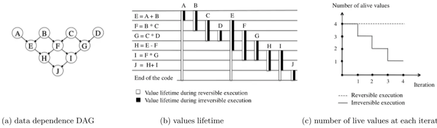
(a) data dependence DAG (b) values lifetime (c) number of live values at each iteration Figure 4: Example comparing number of live values and their lifetime between reversible and irreversible execution
is four. The values computed by independent statements D, E, F and G can all be alive at the same time and thus cannot share registers. Likewise, the values computed by J, K, L and M couldn’t share registers since they are in sep-arate chains, so there is no register reuse between K and M or K and G -contrary to the direct computation, nev-ertheless they are independent and they haven’t the same live range. G and M are indirectly dependent, at the point of use of M, G is already dead and could normally share the same register. But we prevent this, because we need G and I for recomputing F. In this example there are five con-vergences in the graph, which means a loss in information at five points during computing, so we have to save addi-tional information which is one of the inputs at each con-vergence, we can determine a lower bound of the size of this information by finding the minimal number of paths in the minimal decomposition of the reuse DAG. The sets of nodes {A, B, D.H, J, N, P }, {C, F, I, L, O}, {E}, {K}, {G} and {M } are all paths in the graph, and each end of each path can define an information that should be saved for the backward computation. The set of these paths is called register-reuse DAG because all nodes of a path are assigned to the same register. The reuse DAG chains those values that are not simultaneously live and can thus share a register, without any violation of information. Different paths are assigned to different registers, and therefore the number of paths is the number of registers. Thus, the register reuse DAG in figure 3(c) requires at least six registers. Therefore, by The-orem 2 a minimum decomposition of a DAG into elementary paths that don’t contain any sub-path gives a lower bound to the register requirement for a reversible execution.
Theorem 2. The minimum number of registers required for a reversible execution of a program is bigger or equal than the number of elementary paths in a minimal decomposition of the corresponding DAG.
4.
REVERSIBILITY AND VALUES
LIFETIME
There are cases when conventional and reversible computa-tions consume the same number of registers, but values life-time are not the same. As an example, consider the DAG in figure 4(a). Both of the executions -reversible and non-reversible, require 4 registers for the computation. A
regis-ter is used to hold a value from the time that the defining instruction executes until the value is killed by the last in-struction that uses it. Figure 4(b) shows how a value that should be killed and frees a register, stays for the whole computation.
We try to compute the number of live values at every com-putation step. Since we allow only one instruction to be executed at each computation step, the curve is either con-stant or increasing in the reversible computing, figures 4(c) and 5; because we shouldn’t get rid of a value if it’s not directly replaced by another otherwise we will lose unrecov-erable information.
Figure 5: Example comparing the number of live values at each iteration step for the same code in reversible and irreversible execution (corresponding to the code of example 2 figure 3)
This can define another problem in the reversible computing: How to keep the minimum garbage with a shortest lifetime possible? We can deduce the minimum number of registers required for a reversible execution of a program from a direct execution by computing the number of live values at each step. The idea is to add the positive difference of the num-ber of live values between two successive iterations in each computing step. If we take Ψithe number of live values at
the iteration i with i ∈ [1, N - Ψ0] and N is the graph size
or the number of nodes and Ψ0 is the number of sources in
the graph, q is an integer. This simple code can deduct the number of registers required for the reversible execution.
q = Ψ0;
if (Ψi+1− Ψi> 0)
q+ = Ψi+1− Ψi;
In the reversible computing, we should not kill a datum if we have no other way to recompute it unlike in conventional computing. However, each increase of the number of live reg-isters means that new values are generated and no one was killed. The possibility to clean garbage data (garbage-free) to free registers, can be done by a backtrack to recompute intermediate values or the input data.
5.
EXPERIMENTAL RESULTS AND UPPER
BOUND FOR THE GARBAGE SIZE
We come back to our algorithm defined in section 2. In order to understand more about what this criterion of garbage is, we made two kind of experiments. First we generated all graphs of some (small) fixed given size and second we used a randomly generated set of larger graphs. For exhaustive or random generation of DAGs we represent DAGs by their adjacency matrix, namely a boolean matrix with rows and columns labeled by graph vertices, with a 1 or 0 in position (vi, vj) according to whether viand vjis an edge in the DAG
or not. In both cases we computed the garbage as explained in previous sections.
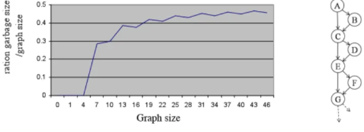
From our experiments of small graphs we exhibited critical graphs for which garbage is maximal. These are the graphs of figure 6(b), where indeed according section 3 garbage is at least n/2 because a partition into elementary paths results in at least n/2 paths if the DAG has n nodes.
(a) garbage size in function of graph size (b) critical graph
Figure 6: upper-bound to the garbage size
In [20] where reversibility of automata instead of DAG is considered, they argue that energetic garbage is related to convergences in automata - that result in loss of information. In this case our critical graphs do not have the maximal number of convergences. Maximal number of convergences correspond to DAG with only binary operations. In our case if we want to maximize the garbage size we have to maximize the number of convergences without increasing the number of register requirement in the direct computation. At least two registers are needed to create a convergence in a graph, so we fix the register requirement to two, and we try to cre-ate a maximum of convergences. We can observe that each increase of the number of convergence of one corresponds to an increase of the graph size of two, which explains the upper-bound of the garbage size (50% of the graph size).
This n/2 upper-bound is actually corroborated by experi-ments on randomly generated larger graphs. Figure 6(a) reports the maximum garbage obtained in percentage of the number of nodes. One can see that this number is never more than 50%.
Figure 7 reports also an histogram of garbage size for differ-ent size of graphs.
Figure 7: Number of graphs randomly generated according to the garbage size
6.
RELATED WORKS AND CONCLUSION
Several works have addressed reversibility at the software level. There are basically two main approaches. Since writ-ing reversible programs by hand is not quite natural, some works are devoted to the design of reversible programming languages [1], [18] Frank’s R [10]. The alternative approach is to convert existing programs written in an irreversible programming language into equivalent reversible programs. An irreversible-to-reversible compiler receives an irreversible program as input and reversibly compiles it to a reversible program.
When one converts irreversible programs into reversible ones one has to face the issue of trading time complexity with data storage complexity. One elegant method was proposed by Bennett [3] where he models the former problem with a pebble game. Pebbles represent available data at some point of the program. One can add pebbles on some node when there is a way to compute that node with data identified by a pebble in a previous node. One can remove pebbles if there is an alternative way to recompute data required in this node. This is therefore an abstraction of reversible compu-tations that allows analysis of the space and time complexity for various classes of problems, but this simulation operates only on sequential list of nodes. This sequence is broken hi-erarchically into sequences ending with checkpoints storing complete instantaneous descriptions of the simulated ma-chine. After a later checkpoint is reached and saved, the simulating machine reversibly undoes its intermediate com-putation, reversibly erasing the intermediate history and re-versibly canceling the previously saved checkpoint. Bennett chose the number of pebbles large enough (n = O(logT )) so that m the number of steps become small. Other works such as [16] have also considered the reversible pebble game. In [22], Vitanyi gives a time-space tradeoff for an irreversible computation using time T and space S to be simulated
re-versibly in time T0 = 3k2O(T /2k)S and space S0
= S(1 + O(k)), where k is a parameter that can be chosen freely 0 ≤ k ≤ log(T ) in order to obtain the required tradeoff between reversible time T0 and space S0. Naumann [21] considers the problem of restoring the intermediate values computed by such a program (the vertices in the DAG) in re-verse order for a given upper bound on the available memory, while keeping the computational complexity to a minimum. He shows that the optimal data-flow reversal problem is NP-complete [21] but he doesn’t consider reversible operations and seeks only reversible behavior for recovering intermedi-ate values in reverse order. Griewank also in [12] presents an optimal time-space tradeoff algorithm in the context of au-tomatic differentiation. In [19] it has been showed that the minimum number of garbage bits required to make a boolean function reversible is dlog(M )e, where M is the maximum of number of times an output pattern is repeated in the truth table. However, traditional techniques for bi-directional ex-ecution are not scalable to all classes of problems.
Conclusion
We have presented an analysis of the number of registers required to make a DAG computing graph reversible. We define the energetic garbage as the additionnal number of registers required for computing a forward and backward execution of the graph with respect to the simple forward execution. We gave a lower bound as the size of the decom-position of the graphs into elementary paths and through our experiments, we found that the garbage size does not exceed 50% of the program size - for DAG of unary/binary operations. However, values lifetime is shorter in a direct computation. A natural followup of this work would be to integrate this register allocation algorithm in a reversible compiler like the RCC -Georgia Tech’s reversible C code compiler [13] in order to compare the size of generated codes with existing reversible programs and memory usage. But we also want to analyse more deeply in computation graphs the data rematerialization for recomputing data instead of reloading from memory - possibly after having spilled them in memory, in the presence and exploitation of reversible operations.
It is amazing to observe that in code optimization on current processors, minimizing power consumption amounts most of the time to minimizing the number of memory accesses, cache misses, etc. Therefore it was quite expectable that this thermodynamics view of computation leads to trade off be-tween storage and recomputing. Understanding more thor-oughly the relationship between variables of a computation graph in terms of mutual information between variables is our next step.
7.
ACKNOWLEDGEMENTS
This work was partially supported by the ANR PetaQCD project. We would like to thank the reviewers for their care-ful reading and very constructive remarks. Unfortunately some of them could not be taken into consideration due to the shortage of time.
8.
REFERENCES
[1] H. G. Baker. NRVERSAL of fortune -the
thermodynamics of garbage collection. Int’l Workshop on Memory Mgmt, 1992.
[2] C. H. Bennett. Logical reversibility of a computation. IBM Journal of Research and Development, 1973. [3] C. H. Bennett. Time-space tradeoffs for reversible
computation. SIAM J. Comput, 1989.
[4] D. Berson, R. Gupta, and M. L. Soffa. Ursa: A unified resource allocator for registers and functional units in vliw architectures. In In Conference on Architectures and Compilation Techniques for Fine and Medium Grain Parallelism, 1992.
[5] D. A. Berson, R. Gupta, and M. L. Soffa. Integrated instruction scheduling and register allocation techniques. In Proc. of the Eleventh International Workshop on Languages and Compilers for Parallel Computing, LNCS, 1998.
[6] P. G. Bishop. Using Reversible Computing to Achieve Fail-safety. IEEE Computer Society, 1997.
[7] S. Burckel and E. Gioan. In situ design of register operations. In ISVLSI ’08: IEEE Computer Society Annual Symposium on Very-Large-Scale Integration, 2008.
[8] S.-K. Chen, W. K. Fuchs, and J.-Y. Chung. Reversible debugging using program instrumentation. IEEE Trans. Softw. Eng., 2001.
[9] R. P. Dilworth. A decomposition theorem for partially ordered sets. Ann. of Math., 1950.
[10] M. P. Frank. The R programming language and compiler. MIT RC Proj. Memo #M8, 1997. [11] M. P. Frank. The physical limits of computing.
Computing in Science and Engg., 2002.
[12] M. Iri, K. Tanabe, K. Academic, and A. Griewank. On automatic differentiation. In in Mathematical
Programming: Recent Developments and Applications, 1989.
[13] k. Perumalla and R. Fujimoto. Source-code transformations for efficient reversibility. Technical Report GIT-CC-99-21, College of Computing, Georgia Tech., 1999.
[14] T. F. Knight, F. R. Morgenthaler, C. J. Vieri, and C. J. Vieri. Pendulum: A reversible computer architecture. Master’s thesis, MIT Artificial Intelligence Laboratory, 1995.
[15] T. Koju, S. Takada, and N. Doi. An efficient and generic reversible debugger using the virtual machine based approach. In VEE ’05: Proceedings of the 1st ACM/USENIX international conference on Virtual execution environments. ACM, 2005.
[16] R. Kr´alovic. Time and space complexity of reversible pebbling. In SOFSEM ’01: Proceedings of the 28th Conference on Current Trends in Theory and Practice of Informatics Piestany, 2001.
[17] R. Landauer. Irreversibility and heat generation in the computing process. IBM Journal of Research and Development, 1961.
[18] C. Lutz and H. Derby. Janus: a time-reversible language. Caltech class project, 1982.
[19] D. Maslov and G. W. Dueck. Reversible cascades with minimal garbage. IEEE Transactions on
Computer-Aided Design of Integrated Circuits and Systems, 2004.
[20] P. Matherat and M. T. Jaekel. Logical Dissipation of Automata Implements - Dissipation of Computation. Technique et Science Informatiques, 1996.
[21] U. Naumann. On optimal DAG reversal. Technical Report AIB-2007-05, 2007.
[22] P. Vit´anyi. Time, space, and energy in reversible computing. In CF ’05: Proceedings of the 2nd conference on Computing frontiers. ACM, 2005. [23] H. Yang, G. R. Gao, and C. Leung. On achieving
balanced power consumption in software pipelined loops. In CASES ’02: Proceedings of the 2002 international conference on Compilers, architecture, and synthesis for embedded systems, 2002.