Coupled seasonal and intraseasonal variability in the South China Sea

Coupled seasonal and intraseasonal

variability in the South China Sea

The MIT Faculty has made this article openly available. Please share

how this access benefits you. Your story matters.

Citation

Wei, Jun et al. “Coupled Seasonal and Intraseasonal Variability in

the South China Sea.” Climate Dynamics 44.9–10 (2015): 2463–2477.

As Published

http://dx.doi.org/10.1007/s00382-014-2250-1

Publisher

Springer Berlin Heidelberg

Version

Author's final manuscript

Citable link

http://hdl.handle.net/1721.1/105149

Terms of Use

Creative Commons Attribution-Noncommercial-Share Alike

DOI 10.1007/s00382-014-2250-1

Coupled seasonal and intraseasonal variability in the South China

Sea

Jun Wei · Dongxiao Wang · Mingting Li · Paola Malanotte‑Rizzoli

Received: 28 December 2013 / Accepted: 2 July 2014 / Published online: 17 July 2014 © Springer-Verlag Berlin Heidelberg 2014

as atmosphere forcing SST. Wind becomes a dominant forcing and demonstrates robust negative relationship with SST and positive relationship with rainfall/LHF. Both coupled and uncoupled models are able to reproduce this observed relationship. In wind-SST relationship, compared to uncoupled and observed variables, the coupled model produced the smallest SST variances and therefore the strongest negative coupling feedback. Sensitivity experi-ments were also carried out to examine the roles of pling by directly comparing differences between the cou-pled and uncoucou-pled experiments with initial temperature perturbations. It is showed that the differences can be up to 50 % of the standard deviations of the variables. Root-mean-square errors of the uncoupled model can be effec-tively reduced by ~65 % in the coupled model.

Keywords Seasonal variability · Intraseasonal

variability · Atmosphere–ocean coupling · Regional coupled model · South China Sea

1 Introduction

The South China Sea (SCS) is the largest marginal sea to the southeast of the Asian continent, extending from 5°N to 25°N and from 100°E to 120°E. The total area of the SCS is about 3,500,000 m2_{, with an average depth of}

~1,200 m and a maximum depth of ~5,500 m. The SCS is a semi-enclosed ocean basin, surrounded by a narrow shelf along the coast of the southern China and a wide continen-tal shelf (Sunda shelf) on its southwest bound (Fig. 1a). It connects in the northeast to the western Pacific through Luzon Strait and in the southwest to the Indonesian seas through Karimata Strait. On one hand, the SCS is rela-tively isolated with remarkable local atmosphere–ocean

Abstract Based on 10 year climatological data and

simu-lations from a regional atmosphere–ocean coupled model (FVCOM-RegCM3), this study examined the coupled sea-sonal and intraseasea-sonal variability of atmospheric–oceanic variables [sea surface temperature (SST), winds, rainfall and heat fluxes] and important roles of coupling in the South China Sea. It is showed that even though both cou-pled and uncoucou-pled models in general are able to capture observed seasonal and intraseasonal variability, the coupled model demonstrates stronger coupling relationship than the uncoupled model. For seasonal variability, the atmosphere– ocean relationship is presented as SST forcing atmos-phere. Atmospheric variables are significantly influenced by strong seasonally-varied SST. The coupled model very accurately reproduced the observed SST variation with a stable equilibrium state, while SST from the uncoupled model gradually drifted away from the equilibrium state lacking of the so-called negative SST-heat flux feedback. Lead-lag analysis showed that the coupled variables dem-onstrated stronger SST-atmosphere relationship than the uncoupled and even observed variables. For intraseasonal variability, the atmosphere–ocean relationship is presented J. Wei (*) · M. Li

Peking University, Beijing, China e-mail: junwei@pku.edu.cn J. Wei · P. Malanotte-Rizzoli

Singapore-MIT Alliance for Research and Technology, Singapore, Singapore

D. Wang

South China Sea Institute of Oceanology, CAS, Guangzhou, China

P. Malanotte-Rizzoli

interactions. On the other hand, situated on the intersection between Pacific and Indian Oceans and between Asian and Australia continents, the SCS is significantly influenced by the adjacent seas, tropical oceans and monsoon sys-tems. Therefore, understanding the atmospheric–oceanic

variability in the SCS is crucial for the regional climate system.

The SCS is a unique ocean basin that affected by four monsoon systems: East Asian monsoon, Indian monsoon, western North Pacific monsoon and Australian monsoon. Fig. 1 Model domains: a

RegCM3 domain with the 50, 200 and 1,000 m isobaths and b FVCOM domain with unstruc-tured grids (Dark gray shading indicates fine triangular grids). The small box marks the SCS domain

It was generally thought that the East Asian summer mon-soon starts in the SCS (Murakami and Matsumoto 1994; Wu and Wang 2000; Wang and Lin 2002), which motivated the South China Sea Monsoon Experiment to study the South China Sea monsoon (Lau et al. 2000). South China Sea monsoon plays an important role on the SCS circula-tions, which was first interpreted by Wyrtki (1961) as oce-anic response to monsoon winds. The SCS circulation, also known as South China Sea Through Flow (SCSTF, Wang et al. 2006a, b, c), transforms cold and salty water of west-ern Pacific through the Luzon Strait into warm and fresh water outflowing through the Karimata Strait (Qu 2000; Fang et al. 2009a; Du and Qu 2010; Xu and Malanotte-Rizzoli 2013). Sea surface temperature (SST) in the SCS is primarily driven by atmospheric heat fluxes (Chen et al. 2003a, b; Lestari et al. 2011) and secondarily by the intru-sion of western Pacific and wind-induced upwelling (Liu and Xie 1999; Liu et al. 2001a). It demonstrates strong seasonal variability due to solar radiation and evaporation cooling (Liu et al. 2001b; Qu 2001) and remarkable intra-seasonal variability due to monsoon winds (Zeng and Wang 2009; Wu 2010). The precipitation and evaporation in the SCS are strongly associated with monsoon winds and SST, with a wet season from June to November and a dry season from December to next April (Jiang and Qian 2000; Wang et al. 2006a, b, c), which in turn shapes the local SST. Sur-face heat and moisture fluxes are also especially important for the SCS (Zeng et al. 2009; Zhang et al. 2012; Wang et al. 2013a), which gains heat from the atmosphere at a rate of ~20–50 W/m2 _{per year and is a recipient of heavy}

rainfall with an annual mean value of ~0.2–0.3 Sv for the entire basin (Qu et al. 2009). For the regional physical oceanography in the SCS, a recent review can be found in Wang et al. (2013b).

The coupling relationship among the atmospheric– oceanic variables in the SCS have been extensively inves-tigated in previous studies, based on the lead-lag analysis (Liu et al. 2004; Wang et al. 2006a, b, c, 1997; Xie et al. 2007; Wu 2010; Sui et al. 2012; Zhang et al. 2012; He and Wu 2013). Using 11 years of space based observations, Liu and Xie (1999) studied the seasonal changes of the mon-soons and oceanic response. They found that wind speed determines the latent heat flux which is a significant fac-tor influencing SST variation, except in the northern SCS where SST variation is affected mostly by winter mon-soons. Based on Hamburg Ocean Atmosphere Parame-ters and Fluxes from Satellite (HOAPS) data, Wang et al. (2006a, b, c) examined EOF distributions of SST, latent and sensible heat fluxes from 1988 to 2002. They found that the three variables are closely associated with monsoon winds. Using climatology records from multiple sources, He and Wu (2013) found that the seasonal SST variation in the SCS is primarily contributed by the net heat flux (NHF)

and secondarily by winds. SST feeds back to precipitation and wind fields by modulating lower-level convergence and atmospheric stability. Based on TRMM and NCEP data, Wu (2010) investigated intraseasonal variations of SST, winds, and heat fluxes. They found that intraseasonal SST changes are mainly induced by winds and rainfall anomalies, and large SST changes may also feedback to atmosphere.

While the previous studies well documented the multi-scale variability among the atmospheric–oceanic variables, most of them were based on climatological data obtained from different datasets, as no any single dataset can pro-vide long-time and complete atmospheric–oceanic vari-ables. For example, as summarized from the previous stud-ies mentioned above, the heat fluxes were obtained from NCEP/OAFlux/ECMWF, rainfall measurements from TRMM/GCPC, winds from NCEP/ECMWF/QuikSCAT and SST from OISST/GISST/SODA. While these variables of different sources can capture a basic pattern of atmos-pheric–oceanic variability, they usually have relative coarse resolutions, and the most importantly, they are not dynami-cally coupled each other. This deficiency may affect the analysis of the atmosphere–ocean relationship, especially for those small-scale interactions in space and time.

On the other hand, the atmosphere–ocean relationship can be examined by means of numerical models which can provide fully-coupled atmospheric–oceanic variables. While most of the numerical studies were based on global models (Wu and Kirtman 2005; Wu et al. 2006; Pegion and Kirtman 2008), the studies using high-resolution regional coupled models are rather less, especially in the SCS. This is probably due to the highly complex topography and bathymetry surrounding the SCS basin which requires a very high resolution of model grids to resolve continen-tal shelf/slope, straits and archipelago. Even though there exist some regional coupled models previously developed in this region, none of them fully resolved the entire SCS and surrounding maritime continents and oceans/seas. Ren and Qian (2005) developed a regional coupled model to simulate the East Asian Summer monsoon. Their model domain excludes almost completely the Indonesian archi-pelago with the southern boundary at 5°S. Fang et al. (2009b) developed a regional coupled model to simulate the summer climate over East Asia. Their domain excludes the Indonesian archipelago and Indian ocean, but includes a large area in the western Pacific ocean, with the southern boundary located at the equator and the western boundary at 100°E. Li and Zhou (2010) developed a regional coupled model over East Asia with a model domain similar to Fang et al. (2009b), but the southern boundary is set on 10°N.

One of major challenges in simulating the climate variability in the SCS is how to represent accurately the local atmosphere–ocean–land interactions and the remote

atmosphere–ocean fluxes transferred from adjacent oceans/ seas into the SCS. Based on an unstructured grid ocean model (FVCOM), Wei et al. (2013) successfully developed a high resolution regional coupled model with a minimum resolution of ~7 km (Fig. 1b), covering the entire SCS, the Indonesian archipelago, and a large section of west-ern Pacific and eastwest-ern Indian Oceans. By comparing with observations, Xu and Malanotte-Rizzoli (2013) examined the ocean component (FVCOM) for two decades (1960s and 1990s) with an emphasis on the ocean states. Com-pared to ocean-only simulations and observations, Wei et al. (2013) validated the fully coupled model with an emphasis on the interannual climate variability in the Mari-time Continent. The present study, based on the same cou-pled model, is going to examine the coucou-pled seasonal and intraseasonal variability in the SCS and important roles of the atmospheric–oceanic coupling.

The rest of the paper is organized as follows. Sec-tion 2 first describes the data used in this study to assess the coupled and the uncoupled model results, followed by brief descriptions of the coupled/uncoupled models, model configuration and experiments. Section 3 describes the seasonal variability from observations and comparisons with the coupled/uncoupled simulations. Section 4 first describes the intraseasonal variability from observations and comparisons with the coupled/uncoupled simulations, followed by analysis of two sensitivity experiments. Sum-mary and discussions are given in Sect. 5.

2 Data and model set‑up

2.1 Data

We used climatological data as a reference to validate the coupled/uncoupled simulations. Similarly, due to the incompleteness of one single dataset, the climatological data were extracted from different sources. Monthly data were used for analysis of seasonal variability, in which SST was from the simple ocean data assimilation (SODA) re-analysis (Carton et al. 2000a, b), surface winds at 10 m, rainfall and heat fluxes from ERA-40 reanalysis. Daily data were used for intraseasonal variability, in which rain-fall measurements and SST were from the Tropical Rain-fall Measuring Mission (TRMM, Huffman et al. 2007)/ Microwave Imager (TMI). Wind data and heat fluxes were from NCEP/NCAR re-analysis (Kalnay et al. 1996). SODA re-analysis is a data assimilation product with a resolu-tion of 2.5° × 0.5° in longitude and latitude in the trop-ics, combining all the worldwide available observations at all ocean depths with the GFDL POP (Parallel Ocean Program) global ocean circulation model for the period 1871–2008 (http://www.atmos.umd.edu/~ocean/). The

ERA-40 re-analysis is provided by the European Cen-tre for Medium-Range Weather Forecasts (ECMWF), with a resolution of 2.5° × 2.5° from 1957 to 2002 (http://apps.ecmwf.int/datasets/). TRMM project is a join mission between NASA and the Japan Aerospace Explora-tion Agency (JAXA) to provide tropical rainfall measure-ments and cloud-penetrating SST maps, with a resolution of 0.25° × 0.25° in longitude and latitude from 1997 to present (http://pmm.nasa.gov/TRMM). The NCEP/NCAR re-analysis is a gridded data set incorporating numeri-cal weather prediction and observations, with a resolution of 2.5° × 2.5° from 1948 to 2008 (http://www.ncep.noaa. gov/).

2.2 The regional atmosphere–ocean coupled model

The atmosphere–ocean coupled model used in this study adopts RegCM3 as the atmospheric component, FVCOM as the oceanic one, and OASIS3 as the coupler. The RegCM3 was originally developed at the National Center for Atmospheric Research (NCAR) and is now maintained by the International Center for Theoretical Physics (ICTP). It includes several options for representing important pro-cesses such as moist convection and land surface physics. The dynamical core of RegCM3 is based on the hydro-static version of the Pennsylvania State University/NCAR Mesoscale Model Version 5 (MM5; Grell et al. 1994) and employs NCAR’s Community Climate Model Version 3 (CCM3) atmospheric radiative transfer scheme (described in Kiehl et al. 1996). Planetary boundary layer dynamics follow the non-local formulation of Holtslag et al. (1990; described in Giorgi et al. 1993). Ocean surface fluxes are handled by Zeng’s bulk aerodynamic ocean flux parameter-ization scheme (Zeng et al. 1998).

The oceanic component of the coupled model is an unstructured grid Finite Volume Coastal Ocean Model (FVCOM), originally developed by Chen et al. (2003b). FVCOM solves the momentum and thermodynamic equa-tions using a second order finite-volume flux scheme, which combines the advantages of finite-element methods for geometric flexibility and finite-difference methods for computational efficiency (Chen et al. 2006a, b). The Mellor and Yamada level 2.5 turbulent closure scheme is used for vertical eddy viscosity and diffusivity (Mellor and Yamada 1982) and the Smagorinsky turbulence closure for horizon-tal diffusivity (Smagorinsky 1963). The most important feature of FVCOM adopted in the coupled model is its flex-ible unstructured grid which allows us to design an effec-tive model grid with varied resolutions according to the complex topography and coastline in the SCS region.

In order to keep synchronization of RegCM3 and FVCOM, the two models were integrated forward simul-taneously managed by the coupler, OASIS3, which

interpolates and transfers the coupling variables of different resolutions from the source grid to the target gird. For more information, please see Wei et al. (2013) who originally developed the coupled model and presented detailed model descriptions and validations.

2.3 Model setup and experiments

The atmosphere domain is set from 85°E to 142°E and from 20°S to 30°N (Fig. 1a). The horizontal resolution is 60 km with 18 uniform vertical sigma layers, from the ground surface to the 50-mb level. The ocean domain covers the entire SCS, Indonesian archipelago, and large sections of the western Pacific and eastern Indian oceans (Fig. 1b). The horizontal resolution varies from ~7 km along the shelf break and in the straits, to ~10 km along the coastlines, to ~50 km over Sunda shelf and deep SCS, and ~200 km along open boundaries. The open eastern and western boundaries have purposely been chosen to be in the two ocean interiors to prevent boundary effects, such as spurious wave reflection, from affecting the SCS. The sigma coordinate is used in the vertical and is configured with 31 layers (finer at surface and coarser at depth). The water depth at each grid is interpolated from the 5-min depth data base ETOPO5.

The model was first spun up from 1960 to 1969. RegCM3 was initialized and forced at boundaries by ECMWF ERA-40 climatology and exchanged surface fluxes every 6 h with FVCOM. FVCOM was initialized using temperature and salinity fields from a global model, MITgcm. The tempera-ture (salinity) at the boundaries was relaxed to the MITgcm simulation. To obtain a stable monsoon circulation, sea level along the open boundaries at the Pacific and Indian Oceans was forced perpetually by weekly SSHA from the MITgcm, and the surface wind was gradually ramped up and updated every 6 h from RegCM3. In addition, to establish a realistic atmosphere–ocean interface thermal structure, a flux cor-rection was used during the model spin-up. Specifically, the SST was relaxed to SODA SST with a depth dependent nudging factor, ranging from 0.2 s−1 _{in shallow water and}

decreasing to 0.001 s−1 _{in the open ocean.}

The coupled and uncoupled simulations of the 1970 to 1979 were used for analysis. The coupled simulation was restarted from the end of the 60 s, but with no SST relaxa-tion applied. The uncoupled simularelaxa-tions were carried out by RegCM3-alone and FVCOM-alone models, restarted from the end of the 60 s as well. The configuration of the RegCM3-alone model is the same as the coupled RegCM3, except that the ocean SST is prescribed by GISST re-anal-ysis. Similarly, the FVCOM-alone model adopted the same configuration as the coupled FVCOM, except that the sur-face fluxes are prescribed by the fluxes from the RegCM3-alone simulations.

3 Seasonal variability in the SCS

3.1 Comparison of observed and simulated atmospheric– oceanic variables

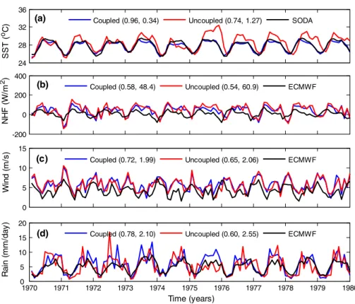
Due to seasonal south–north progression of the Sun over the tropical region, all atmospheric–oceanic variables in the SCS demonstrate prominent seasonal variability. Figure 2 shows evolutions of monthly SST, NHF, wind speed and rainfall averaged over the SCS domain from coupled/uncoupled simulations, and from observations. The observed SST is from SODA, and the observed atmospheric variables from ECMWF ERA40. All variables demonstrate dominant sea-sonal cycles in the first order, and notable intraseasea-sonal wig-gles in the second order, especially for winds and rainfall. To assess the coupled/uncoupled results, correlation coefficients (R) and root mean square errors (RMSE) between model variables and observed ones are also presented in Fig. 2.

Among all the variables, the coupled SST is in the best agreement with observations (R = 0.96 and RMSE = 0.34 °C). Uncoupled SST, driven by prescribed heat fluxes, gradually drifts away from the climatology state with a downgraded correlation coefficient (R = 0.74) and higher RMSE of 1.27 °C. NHF, representing 4 heat flux components: latent heat, sensible heat, long-wave radiation and short-wave solar radiation, is the most impor-tant forcing to modulate SST, which can in turn influence the 4 components. Compared to the observed NHF, the model NHFs are slightly overestimated, while the differ-ence between coupled/uncoupled NHFs is very small in terms of values of R and RMSE. The evolutions of cou-pled/uncoupled winds are in a reasonable good agreement with observed winds (R = 0.72 for coupled and 0.65 for uncoupled). However, the coupled/uncoupled winds again are slightly overestimated compared to observed winds. While both coupled and uncoupled models are able to simulate the seasonality of rainfall with reasonable R and RMSE (R = 0.78 for coupled and 0.6 for uncoupled), the difference between the model and observed rainfall is nota-ble. The model rainfall generally shows higher rainfall and more intraseasonal wiggles than observed one. This is likely due to high resolution of model grids, which resolves more details of mountains around the SCS basin.

Improvement of the coupled simulation over the uncoupled one is also prominent in horizontal views. Figure 3 shows dif-ferences between coupled/uncoupled variables and observed ones of 1970–1979 in the SCS. With prescribed SST, the uncoupled model (RegCM3-alone) produces abnormally high NHF over the southern SCS and along the northern shelf of the SCS (Fig. 3b), which results in warm bias in the uncoupled SST (Fig. 3a). The uncoupled wind shows a systematically overestimation of wind speed (up to 2 m/s) all over the entire SCS domain but with large values basically along the coast

(Fig. 3c). The discrepancy may come from model parameteri-zation, ocean SST condition and resolution as well. Further, the uncoupled rainfall produces wet bias in the northern SCS and dry bias in the southern SCS. The maximum bias is gener-ally located near coast, to the west of Philippine islands and the Borneo island (Fig. 3d), indicating that the rainfall bias is most likely due to the land/mountain effects. On the other hand, the coupled model overall improve the uncoupled simu-lations to different extents, for example, more effectively for SST and NHF and less for winds and rainfall, more improve-ment over the SCS basin and less near the coast.

3.2 Comparison of EOFs of observed and simulated variables

To further understand the seasonal variability of observed and model variables and the coupling relationship, we compared their spatial distributions of empirical orthogo-nal function (EOF) and corresponding principal compo-nent (PC). Figure 4 shows the 1st EOF modes of observed SST, NHF, wind speed and rainfall, and the same variables from the coupled and uncoupled simulations. The EOFs of all variables were calculated based on monthly mean from 1970 to 1979. Since the units of the variables are different, all variables were de-mean and normalized by their stand-ard deviations before calculating the EOFs.

In Fig. 4a, the 1st EOF modes of SST account for 88.4, 64.6 and 82.2 % of total variance for SODA, uncoupled and

coupled SST, indicating their dominant seasonality. For SODA SST, the spatial distribution shows prominent high variances along the northern shelf of the SCS, with a tongue extending southward along the coast of Vietnam. The variances gradu-ally decrease to zero near the equator. The distribution of the uncoupled SST, however, shows a very high variance (>0.06) in the gulf of Beibu, and high variances to the west of Luzon strait and over the Sunda shelf. The coupled model improves the uncoupled one by increasing the variance west of the Luzon strait and decreasing the variance in the southern SCS. It is noted that the low variance along the northern shelf in the model is due to persistent cold water intruded from Taiwan strait, which is not presented in the SODA SST.

In Fig. 4b, the 1st EOFs of NHF account for 78.2, 65.2 and 65.1 % of total variance for ECMWF, uncoupled and coupled NHF. The distributions of observed and model NHF are similar with a north–south pattern similar to SST (Fig. 4b), which is obviously associated with the north– south progression of solar radiation. The general north– south distribution of NHF and SST indicates a strong NHF–SST forcing relationship, in which the solar radia-tion of the Sun is the most important factor to drive SST changes. Compared to the observed NHF, the uncoupled model underestimates the variance along the northern shelf, while the coupled model greatly increases the variance through SST–NHF feedback. Intruded cold water from the Taiwan strait suppresses ocean evaporation and latent heat flux, and therefore enhances NHF.

Fig. 2 Evolution of domain-averaged a SST, b NHF, c winds and d rainfall in the SCS for coupled/uncoupled simulations and observations. The first and second values in parentheses are correlation coefficient and root-mean-square error (RMSE) between the simulated and observed variables 24 28 32 36 SST ( oC)

(a) Coupled (0.96, 0.34) Uncoupled (0.74, 1.27) SODA

1970 1971 1972 1973 1974 1975 1976 1977 1978 1979 1980 0 5 10 15 20 Time (years) (d) Ra in (m m/ da y)

Coupled (0.78, 2.10) Uncoupled (0.60, 2.55) ECMWF -200 0 200 400 (b) NHF (W /m 2)

Coupled (0.58, 48.4) Uncoupled (0.54, 60.9) ECMWF

0 5 10 15 Wi nd (m /s )

In Fig. 4c, the 1st EOFs of winds account for 65.8, 47.2 and 50.8 % of total variance for ECMWF, uncoupled and coupled winds. The distribution of ECMWF winds shows a

high variance west of the Luzon strait extending all the way to the southern SCS, and gradually decreases towards coast and the equator. However, the uncoupled wind shows a Fig. 3 Differences of

uncou-pled/coupled simulations and observations for a SST, b NHF, c Wind speed and d Rainfall in the SCS for decade of 1970s

0 5 10 15 20 25 (a) SST 0 5 10 15 20 25 -2 -1 0 1 2 0 5 10 15 20 25 (b) NHF 0 5 10 15 20 25 -150 -100 -50 0 50 100 150 0 5 10 15 20 25 (c) Wind 0 5 10 15 20 25 -4 -2 0 2 4 100 105 110 115 120 125 0 5 10 15 20 25 (d) Rain 100 105 110 115 120 125 0 5 10 15 20 25 -5 0 5

different pattern with a maximum of variance in the south-ern SCS. The main discrepancy of observed and uncou-pled results is in the northern SCS, which is probably due to the effects of the Taiwan and Philippines islands which are not resolved in ECMWF given its 2.5º resolution. The coupled winds generally is similar to the uncoupled one but with some improvement right above the Borneo island and to the west of the Philippine islands using ECMWF as a reference.

In Fig. 4d, the 1st EOFs of the rainfall account for 58, 36.9 and 33 % of total variance for ECMWF, uncoupled and coupled rainfall. The observed rainfall shows high

variances over the central SCS basin with a maximum located 200 km to the west of the Philippines islands. In contrast, the uncoupled model shows a very high variance of rainfall right on the west of the Philippines islands and zero variance in the southern SCS, which again is likely due to the effects of Taiwan/Philippines islands. On the other hand, the coupled model suppresses the rainfall maxi-mum on the west of the Philippines islands, and overall increases slightly the rainfall in the entire SCS basin.

While we used ECMWF reanalysis as reference, they incorporated measurements from different sources and their resolutions cannot fully resolve the details of islands/

0 5 10 15 20 25 (a) SODA (88.4%) 0 5 10 15 20 25 Uncoupled (64.6%) 0 5 10 15 20 25 Coupled (82.2%) 0 0.02 0.04 0.06 0 5 10 15 20 25 (b) ECMWF (78.2%) 0 5 10 15 20 25 Uncoupled (65.2%) 0 5 10 15 20 25 Coupled (65.1%) 0 0.02 0.04 0.06 0 5 10 15 20 25 (c) ECMWF (65.8%) 0 5 10 15 20 25 Uncoupled (47.2%) 0 5 10 15 20 25 Coupled (50.8%) 0 0.02 0.04 0.06 100 105 110 115 120 125 0 5 10 15 20 25 (d) ECMWF (58.0%) 100 105 110 115 120 125 0 5 10 15 20 25 Uncoupled (36.9%) 100 105 110 115 120 125 0 5 10 15 20 25 Coupled (33.0%) 0 0.02 0.04 0.06

mountains around the SCS. The coupled model, even though contains model deficiency, can provide dynamically coupled variables and uncoupled variables by turning off the pling to investigate the roles of the atmosphere–ocean cou-pling from their lead-lag relationship. Figure 5 shows decadal averaged annual cycles of the 1st PC between SST and the atmospheric variables: NHF, LHF, wind speed and rainfall for observations and coupled/uncoupled simulations. It is clearly showed that NHF leads SST for all three cases, confirming the NHF–SST forcing relationship (Fig. 5a). However, the lead-ing time is different, about 2 months for observed NHF–SST, 1.5 months for the uncoupled one and less than 1 month for the coupled one. The observed LHF leads SST by 2 months, the same phase with the NHF, and the observed wind leads SST by 1 month (Fig. 5b). In contrast, the model winds are almost coincident with model LHF, however, the uncoupled wind/LHF leads SST about 1.5 months and the coupled wind/LHF is almost in the same phase with the SST. On the other hand, the observed rainfall lags SST about 1 month and the coupled model shows the similar relationship (Fig. 5c).

The uncoupled rainfall, however, lags SST in its onset season of March to June and leads SST in its retreat season of Sep-tember to December. Figure 5 indicates an atmosphere–ocean relationship of SST forcing atmosphere for seasonal variabil-ity in the SCS. The seasonal change of ocean SST, primarily driven by north–south progression of solar radiation, greatly influences the evolution of monsoon winds, rainfall, LHF and therefore NHF, which in turn modulates the ocean SST. Over-all, the coupled variables show a faster atmosphere–ocean response time than the uncoupled and observed ones.

4 Intraseasonal variability in the SCS

4.1 Intraseasonal variability of observed variables

The first EOF modes of the observed and model variables demonstrated dominant seasonal variability, while we also noticed remarkable intraseasonal variability shown as wiggles in Fig. 2. In this section we will focus on the -2 -1 0 1 2 (a) Observations SST NHF Uncoupled Coupled -2 -1 0 1 2 (b) SST Wind LHF J F M A M J J A S O N D -2 -1 0 1 2 (c) SST Rain J F M A M J J A S O N D Time (months) J F M A M J J A S O N D

Fig. 5 Average annual cycles of principal components of SST versus a NHF, b winds and LHF, and c rainfall from observations and coupled/ uncoupled simulations

intraseasonal variability. To extract the intraseasonal anom-aly, we used daily mean of the variables instead of the monthly mean. For SST, SODA only provides monthly SST; TRMM/TMI provides daily SST but it starts from 1997. For atmospheric variables, the ECMWF ERA-40 project ends on 2002 and NCEP is from 1948 to 2008. Given the incompleteness of these datasets, for intra-seasonal comparison we chose SST from TRMM/TMI in 1998–2007 and atmospheric variables from NCEP in the same period as a reference. Climatology and seasonal trend were removed from the daily means of the variables, in which climatology was defined as 10-year mean and the seasonal trend as a 60-day running mean.

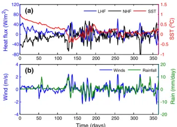
Figure 6 shows intraseasonal variations of observed winds against rainfall, SST and LHF of the year of 1998. It is showed that the intraseasonal variations of the atmospheric– oceanic variables demonstrate remarkable correlations in time scales of ~10 days. In Fig. 6a, the rainfall anomaly is small from January to April (dry season), and rapidly increases at about day 130, which is so-called SCS summer monsoon (SCSSM) onset. After the SCSSM onset, the evo-lution of the rainfall anomaly is highly coincident with wind anomaly, indicating a positive wind-rainfall relationship. In Fig. 6b, SST anomaly in general evolves inversely with the wind anomaly. Negative wind anomalies accompany SST warming, and positive wind anomalies coincide with rapid SST cooling. In Fig. 6c, LHF anomaly basically follows the wind anomaly, especially after the SCSSM. NHF anomaly is very similar to the LHF (not shown). This relationship indi-cates a relationship of atmosphere forcing SST: wind-evapo-ration-rainfall-NHF–SST mechanism. On one hand, positive wind anomaly enhances evaporation and LHF. On the other hand, it enhances convective rainfall and cloud coverage. Both decrease NHF and successively the ocean SST.

4.2 Comparison of observed and simulated intraseasonal variability

Figure 6 shows reliable positive wind-rainfall-LHF and negative wind-SST in observations. Since the observed variables are in the different period with model simula-tions, we are not going to directly compare the evolution of the variables, but statistics of their relationship. To quan-tify the relationship among the variables, variance ellipses with orientation and ellipticity were calculated using EOF. The variance ellipse between two correlated variables is determined by semi-major and semi-minor axes which are the first and second EOF modes of the variables. The orientation of the ellipse is defined as the angle between the semi-major axis and x axis, and ellipticity is the ratio of semi-minor and semi-major axes. To unify the vari-ables of different units, SST, wind, LHF and rainfall were normalized respectively by 1.09, 4.03, 205.5 and 10.9 which are standard deviations of the observed variables of 1998–2007.

Figure 7 shows scatter plots of rainfall, wind-SST, wind-LHF and the corresponding variance ellip-ses of observed variables in 1998 and coupled/uncoupled variables in 1970. Orientation angle and ellipticity of the corresponding ellipse are marked in each plot. In Fig. 7a, the orientation of the observed wind-rainfall (O = 39°) indicates the positive wind-rainfall relationship, and the ellipticity (E = 0.39) indicates the degree of linear rela-tionship (1—circle and 0—line). Generally, both coupled and uncoupled models are able to accurately reproduce the observed wind-rainfall relationship in terms of orien-tation and ellipticity. The difference between the coupled/ uncoupled simulations is very little. In Fig. 7b, the negative observed wind-SST relationship is also well reproduced by model simulations, but the uncoupled ellipse with O = −38 and E = 0.7 indicates higher SST variances (weak SST constraint) than observed one and the coupled wind-SST shows the strongest wind-wind-SST constraint. In Fig. 7c, while the models also reproduce the positive wind-LHF relationship, the model shows much stronger wind-LHF relationship than observed one.

Figure 8 summarizes the statistics of orientation angle and ellipticity of observed variables for 1998–2007 and model variables for 1970s. For wind-rainfall, the observa-tions and simulaobserva-tions are very similar in terms of orienta-tion and ellipticity over the 10 years, indicating a very robust relationship between wind and rainfall anomalies. For wind-SST, coupled variables show overall smallest orientation angle (smallest SST variances) compared to uncoupled and observed ones. This is reasonable as the coupled SST is constrained more effectively by atmos-pheric variables through the wind-evaporation-rainfall-NHF–SST negative feedback. The orientation angles of the -5 0 5 Wi nd (m /s ) 0 50 100 150 200 250 300 350 -12 12 Rain (mm/day) -5 0 5 Wi nd (m /s ) 0 50 100 150 200 250 300 350 -2 -1 0 1 2 SST ( oC) -5 0 5 Wi nd (m /s ) Time (days) 0 50 100 150 200 250 300 350 -300 0 300 Latent (W/m 2) Wind SST LHF Rain (a) (b) (c)

Fig. 6 Observed intraseasonal variations of winds against a rainfall, b SST and c LHF in the SCS in the year of 1998

Fig. 7 Scatter plots and associ-ated ellipses for a wind-rainfall, b wind-SST and c wind-LHF for observed variables of 1998 and for coupled/uncoupled variables of 1970. Note that all variables are normalized by the standard deviation of observed variables of 1998–2007. The first and second values in paren-theses are rotation angles and ellipticity -1 0 1 Rainfall (mm/day) (a) (39, 0.39) Observations -1 0 1 (b) (-27, 0.6) SST ( oC) -1 0 1 -1 0 1 Wind (m/s) (c) (41, 0.62) LHF (W/m 2) Uncoupled (40, 0.4) (-38, 0.7) -1 0 1 Wind (m/s) (20, 0.17) Coupled (41, 0.45) (-20, 0.61) -1 0 1 Wind (m/s) (17, 0.18) 1 2 3 4 5 6 7 8 9 10 0 50 100 Wind-Rain Orientation (degree)

(a) Obs. Uncoupled Coupled

1 2 3 4 5 6 7 8 9 10 -100 -50 0 Wind-SST 1 2 3 4 5 6 7 8 9 10 0 50 100 Wind-LH F Time (years) 1 2 3 4 5 6 7 8 9 10 0 0.5 1 Ellipticity (b) 1 2 3 4 5 6 7 8 9 10 0 0.5 1 1 2 3 4 5 6 7 8 9 10 0 0.5 1 Time (years)

Fig. 8 Statistics of variance ellipses for a Orientation and b Ellipticity for observed variables of 1998–2007 and for coupled/uncoupled variables of 1970s

uncoupled variables are overall the largest as the uncoupled model which completely excludes the atmosphere–ocean constraint. On the other hand, the coupled wind-SST shows a consistently smaller ellipticity (higher linearity) than the uncoupled one. For wind-LHF, the 10-year statistics of var-iance ellipse confirms a stronger model wind-LHF relation-ship than the observed one.

4.3 Roles of atmosphere–ocean coupling

The difference between the coupled and uncoupled simula-tions demonstrates the roles of atmosphere–ocean coupling. Figure 9 compares differences of SST, NHF, wind speed, LHF, rainfall and divergence of wind fields between the coupled/uncoupled simulations. In Fig. 9a, SST difference is up to 1 °C which accounts for about 50 % of the intrasea-sonal SST anomaly. NHF difference is highly coincident with SST and leads SST by a few days. Wind difference is highly coincident with LHF but is opposite to SST/NHF. Rainfall difference is coincident with the wind/LHF but is opposite to wind divergence. These results indicate a SST-wind-evaporation-rainfall-NHF coupling mechanism. On one hand, the SST difference changes wind/LHF, and then NHF which in turn changes SST as well. On the other hand, the SST difference influences wind divergence and then rainfall. In Fig. 9c, positive SST difference corre-sponds to wind divergence and less rainfall, and vice versa. To further examine the SST influences on the atmos-pheric variables, we carried out two SST perturbation experiments to observe responses of the atmospheric vari-ables. Experiment #1 is an uncoupled model run in which the prescribed SST is persistently increased by 1 °C. Experiment #2 is a coupled model run in which the ini-tial model temperature is increased at all-depth by 1 °C. Figure 10 shows the evolution of the difference between the experiment #1 and the reference experiment without

perturbations. With increased SST of 1 °C, LHF is immedi-ately enhanced and remains positive over most time of the year with a mean value of 30 W/m2_{, while NHF is}

nega-tive with an opposite phase to LHF and a mean value of

−45 W/m2. On the other hand, increased SST enhances wind and rainfall as well, with a mean of 0.84 m/s and 4.5 mm/day respectively over the year. Noted that wind is again highly coincident with rainfall in this case.

The result of experiment #2, shown in Fig. 11, is much different from the experiment #1. At day 0, LHF is enhanced to 38 W/m2 _{and NHF is about −45 W/m}2_,

indi-cating that NHF is mostly dominated by LHF component. NHF gradually increases as LHF decreases with time. Due to negative NHF, SST gradually decreases as well from day 0 to 130. In this period, SST is basically modulated by the NHF–SST feedback, while wind and rainfall are not very sensitive to the SST perturbation. At day 130, roughly the Fig. 9 Differences between

coupled and uncoupled simula-tions in 1970: a SST (black

line) and NHF (bars), b wind (black line) and LHF (bars), c Rainfall (black line) and wind divergence (bars). Note that NHF, LHF and wind divergence are scaled to match the SST, wind and rainfall variances.

Blue and red colors denote posi-tive/negative values -2 0 2 SST ( oC) (a) -4 -2 0 2 4 Wind (m/s) (b) 0 50 100 150 200 250 300 350 -10 0 10 Rain (mm/day) (c) Time (days) -200 0 200 400 (a) Heat flux (W/m 2) 0 50 100 150 200 250 300 350 -1 0 1 2 SST ( oC) -8 -4 0 4 8 Wind (m/s ) Time (days) 0 50 100 150 200 250 300 350 -40 -20 0 20 40 Rain (mm/day) Winds Rainfall LHF NHF SST (b)

Fig. 10 Evolution of the difference of a SST versus LHF/NHF and b wind versus rainfall between the new experiment # 1 and the refer-ence experiment

time of the SCS summer monsoon onset, the wind/rainfall increases suddenly, resulting in a rapid decrease of NHF and SST. After day 130, wind/rainfall starts oscillating with a ~10 day period and SST is mainly controlled by the wind-evaporation-rainfall-SST feedback described in the Sect. 4.1. The RMSE of the coupled variables are 15, 22, 0.72, 2.63 for LHF, NHF, winds and rainfall respectively, and account for 35.5, 48.2, 34.8 and 35.1 % of the uncoupled ones. In another word, the coupled model bias is reduced by ~65 % compared to the uncoupled model. It is noted that in the experiment #2 the responses of the atmospheric variables to the SST perturbation can be divided into two stages: stage of SST forcing atmosphere from day 0 to day 130 (seasonal scale), and stage of atmospheric forcing SST after day 130 (intraseasonal scale).

5 Summary and discussions

Based on 10 year climatological data and simulations from a high resolution regional atmosphere–ocean cou-pled model, this study examined the coucou-pled seasonal and intraseasonal variability of atmospheric–oceanic variables (SST, winds, rainfall and heat fluxes) in the SCS and roles of coupling in the atmospheric–oceanic relationship. Model variables were first assessed against the observations. It is showed that both coupled and uncoupled models in general are able to capture the observed seasonal and intraseasonal variability, while the coupled model demonstrated stronger atmosphere–ocean relationship than the uncoupled one and even the observations in some aspect. For seasonal variabil-ity, atmosphere–ocean relationship in the SCS is presented as SST forcing atmosphere. Seasonal variation of SST strongly influences winds, rainfall, latent heat fluxes. The atmospheric variables in turn can modulate SST to some extent. For intraseasonal variability, the atmosphere–ocean relationship is presented as atmosphere forcing SST. Intra-seasonal wind anomaly shows reliably positive relationship with rainfall and latent heat flux, and negative relationship with SST.

In the comparison of the seasonal variations, model vari-ables showed different degree of agreement with observa-tions. The coupled SST is in the best agreement with SODA SST among all variables. This is likely due to the success-ful model spin-up in which the coupled model SST was relaxed to SODA SST for 10 years of 1960s. In the simu-lation of 1970s, the negative feedback between the atmos-phere–ocean variables constrains the coupled SST towards a stable equilibrium state. On the other hand, initialized with the same ocean condition but driven by prescribed heat fluxes, the uncoupled SST gradually drifted away from the equilibrium state without constraint of the atmosphere– ocean feedback. All model atmospheric variables were

consistently overestimated compared to observed ones, which may be partially due to the difference of resolution of observations (2.5° × 2.5°) and model grid (60 km) and partially the model bias. Overall, to some extend the cou-pled atmospheric variables outperform the uncoucou-pled ones with better correlation coefficients and smaller root-mean-square errors (RMSE) with observations. In the compari-son of the EOFs, the coupled variables show shorter lead/ lag time compared to the uncoupled and observed ones (Fig. 6). This indicates that the coupled variables respond much quickly in the fully coupled model, while the uncou-pled and observed variables represent their own variability without a dynamical feedback.

In the comparison of the intraseasonal variations, given incompleteness of climatological dataset and the reliable relationship of atmosphere–ocean variables in the SCS as shown in previous studies, we compared the statistics of the model relationship of 1970s with observations of 1998– 2007. Generally, the coupled and uncoupled models are able to reproduce the observed atmosphere–ocean relation-ship. For wind-SST relationship, the orientation angles of the coupled simulation are overall smaller than the uncou-pled one, indicating a smaller variance of couuncou-pled SST due to the constraint of the atmosphere–ocean feedback. For wind-LHF relationship, the observed variables show much weaker relationship than the simulated ones (Fig. 8). This is probably due to the fact that (1) the winds and LHF data are not dynamically coupled, and (2) the model overes-timates influence of winds on LHF which can be signifi-cantly affected by SST and relative humidity as well.

While observed/re-analysis variables, extracted from dif-ferent climatology datasets, were used as references in this study, they are not fully coupled indeed and usually with rela-tive coarse resolutions. The difference between the coupled

-80 -40 0 40 80 120 Heat flux (W/m 2) -4 -2 0 2 4 Wind (m/s ) Time (days) 0 50 (a) (b) 100 150 200 250 300 350 -1 -0.5 0 0.5 1 1.5 0 50 100 150 200 250 300 350 -20 -10 0 10 20 Winds Rainfall LHF NHF SST SST ( oC) Rain (mm/day)

Fig. 11 Evolution of the difference of a SST versus LHF/NHF and b wind versus rainfall between the new experiment # 2 and the refer-ence experiment

simulation and the observations is not only due to the model bias but also due to the deficiency of the observations. The improvement of the coupled model over the uncoupled model is significant, especially for SST and heat fluxes. The actual differences of coupled and uncoupled SST can be up to 50 % of the standard deviations of their intraseasonal variances (Fig. 9a). On the other hand, the sensitivity experiments with SST perturbation suggested that initial SST bias can spread to atmospheric variables, while RMSEs of the coupled model with the same initial SST perturbation are effectively reduced by about 65 % compared to the uncoupled model.

Acknowledgments This study was supported jointly by National Natural Science Foundation of China (No. 41106003), the Strategic Priority Research Program of the Chinese Academy of Sciences (No. XDA11010303) and by the Singapore National Research Founda-tion (NRF) through Center for Environmental Sensing and Monitor-ing (CENSAM) under the SMonitor-ingapore-MIT Alliance for Research and Technology (SMART) program.

References

Carton JA, Chepurin G, Cao X, Giese BS (2000a) A simple ocean data assimilation analysis of the global upper ocean 1950–1995, part 1: methodology. J Phys Oceanogr 30:294–309

Carton JA, Chepurin G, Cao X (2000b) A simple ocean data assimi-lation analysis of the global upper ocean 1950–1995. Part 2: results. J Phys Oceanogr 30:311–326

Chen JM, Chang CP, Li T (2003a) Annual cycle of the South China Sea surface temperature using the NCEP/NCAR reanalysis. J Meteorol Soc Jpn 81(4):879–884

Chen C, Liu H, Beardsley RC (2003b) An unstructured, finite-volume, three-dimensional, primitive equation ocean model: application to coastal ocean and estuaries. J Atmos Oceanic Tech 20:159–186 Chen C, Beardsley RC, Cowles G (2006a) An unstructured grid,

finite-volume coastal ocean model-FVCOM user manual. School for Marine Science and Technology, University of Massachusetts Dartmouth, New Bedford, Second Edition. Technical Report SMAST/UMASSD-06-0602

Chen C, Beardsley RC, Cowles G (2006b) An unstructured grid, finite-volume coastal ocean model (FVCOM) system. Spe-cial Issue entitled “Advance in Computational Oceanography”. Oceanography 19(1):78–89

Du Y, Qu T (2010) Three inflow pathways of the Indonesian through-flow as seen from the simple ocean data assimilation. Dyn Atmos Oceans 50:233–256

Fang G, Wang Y, Wei Z, Fang Y, Qiao F, Hu X (2009a) Interocean cir-culation and heat and freshwater budgets of the South China Sea based on a numerical model. Dyn Atmos Oceans 47:55–72 Fang Y, Zhang Y, Tang J, Ren X (2009b) A regional air-sea coupled

model and its application over East Asia in the summer of 2000. Adv Atmos Sci. doi:10.1007/s00376-009-8203-7

Giorgi F, Marinucci MR, Bates GT (1993) Development of a second-generation regional climate model (RegCM2). Part I: bound-ary-layer and radiative transfer processes. Mon Weather Rev 121:2794–2813

Grell GA, Dudhia J, Stauffer DR (1994) Description of the fifth generation Penn State/NCAR Mesoscale Model (MM5), Tech-nical Report TN-398+ STR. National Center for Atmospheric Research, Boulder

He ZQ, Wu RG (2013) Coupled seasonal variability in the South China Sea. J Oceanogr 69:57–69. doi:10.1007/s10872-012-0157-1

Holtslag AAM, de Bruijn EIF, Pan H-L (1990) A high-resolution air mass transformation model for short-range weather forecasting. Mon Weather Rev 118:1561–1575

Huffman GJ, Adler RF, Bolvin DT, Gu G, Nelkin EJ, Bowman KP, Hong Y, Stocker EF, Wolff DB (2007) The TRMM multi-satellite precipitation analysis: quasi-global, multi-year, combined-sensor precipitation estimates at fine scale. J Hydrometeorol 8:38–55 Jiang J, Qian Y (2000) The general character of precipitation over the

South China Sea. ACTA Meteorol Sin 58(1):60–69

Kalnay E, Kanamitsu M et al (1996) The NCEP/NCAR 40-year rea-nalysis project. Bull Am Meteorol Soc 77:437–471

Kiehl JT, Hack JJ, Bonan GB, Boville BA, Breigleb BP, Williamson DL, Rasch PJ (1996) Description of the NCAR Community Cli-mate Model (CCM3). In: NCAR technical note TN-420+ STR. h ttp://www.cgd.ucar.edu/cms/ccm3/TN-420/

Lau KM, Ding YH, Wang JT, Johnson R, Keenan T, Cifelli R, Gerlach J, Thiele O, Rikenback T, Tay SC, Lin PH (2000) A report of the field operations and early results of the South China Sea Monsoon Experiment (SCSMEX). Bull Am Meteorol Soc 81:1261–1270 Lestari RK, Watanabe M, Kimoto M (2011) Role of atmosphere–

ocean coupling in the interannual variability of the South China Sea summer monsoon. J Meteorol Soc Jpn 89A:283–290 Li T, Zhou GQ (2010) Preliminary results of a regional air-sea

cou-pled model over East Asia. Chinese Sci Bull 55. doi:10.1007/ s11434-010-0071-0

Liu WT, Xie XS (1999) Spacebased observations of the seasonal changes of South Asian monsoons and oceanic responses. Geo-phys Res Lett 26(10):1473–1476

Liu QY, Yang HJ, Liu ZY (2001a) Seasonal feature of the Sverdrup circulation in the South China Sea. Prog Nat Sci 11(3):202–206 Liu Z, Yang H, Liu Q (2001b) Regional dynamics of seasonal

vari-ability in the South China Sea. J Phys Oceanogr 31:272–284 Liu QY, Jiang X, Xie SP, Liu WT (2004) A gap in the Indo-Pacific

warm pool over the South China Sea in boreal winter: sea-sonal development and interannual variability. J Geophys Res 109:C07012. doi:10.1029/2003JC002179

Mellor GL, Yamada T (1982) Development of a turbulence closure model for geophysical fluid problem. Rev Geophys Space Phys 20:851–875

Murakami T, Matsumoto J (1994) Summer monsoon over the Asian con-tinent and western North Pacific. J Meteorol Soc Jpn 72:719–745 Pegion K, Kirtman B (2008) The impact of air–sea interactions

on the simulation of tropical intraseasonal variability. J Clim 21:6616–6635

Qu T (2000) Upper-layer circulation in the South China Sea. J Phys Oceanogr 30:1450–1460

Qu TD (2001) Role of ocean dynamics in determining the mean sea-sonal cycle of the South China Sea surface temperature. J Geo-phys Res 106(C4):6943–6955

Qu T, Song YT, Yamagata T (2009) An introduction to the South China Sea through-flow: its dynamics, variability and application for climate. Dyn Atmos Oceans 47:3–14

Ren X, Qian Y (2005) A coupled regional air–sea model, its perfor-mances and climate drift in simulation of the east Asian summer monsoon in 1998. Int J Climatol 25:679–692

Smagorinsky J (1963) General circulation experiments with the primitive equations. I. The basic experiment. Mon Weather Rev 91:99–164

Sui D, Xie Q, Wang D (2012) A discuss on interannual to decadal variations of latent heat exchange over the South China Sea. Acta Oceanol Sin 34(4):27–34

Wang B, Lin Ho (2002) Rainy season of the Asian-Pacific summer monsoon. J Clim 15:386–398

Wang DX, Qin ZH, Zhou FX (1997) Study on air–sea interaction on the interannual time-scale in the South China Sea. Acta Meteorol Sin 55(1):33–42

Wang C, Wang W, Wang D, Wang Q (2006a) Interannual variability of the South China Sea associated with El Nino. J Geophys Res 111:C03023. doi:10.1029/2005JC003333

Wang D, Liu Q, Huang R et al (2006b) Interannual variability of the South China Sea throughflow inferred from wind data and an ocean data assimilation product. Geophys Res Lett 33:14. doi:10. 1029/2006GL026316

Wang G, Huang W, Wang H (2006c) Study on the temporal and spa-tial variability of atmosphere–ocean flux over South China Sea with HOAPS data. Acta Oceanol Sin 28(4):1–8

Wang D, Zeng L, Li X, Shi P (2013a) Validation of satellite-derived daily latent heat flux over the South China Sea, compared with observations and five products. J Atmos Ocean Technol 30:1820–1832

Wang D et al (2013b) Progress of regional oceanography study asso-ciated with western boundary current in the South China Sea. Chin Sci Bull 58(11):1205–1215

Wei J, Malanotte-Rizzoli P, Eltahir EAB, Xue P, Xu D (2013) Cou-pling of a regional atmospheric model (RegCM3) and a regional ocean model (FVCOM) over the Maritime Continent. Dyn Clim.

doi:10.1007/s00382-013-1983-6

Wu RG (2010) Subseasonal variability during the South China Sea summer monsoon onset. Clim Dyn 34:629–642. doi:10.1007/ s00382-009-0679-4

Wu R, Kirtman B (2005) Roles of Indian and Pacific Ocean air– sea coupling in tropical atmospheric variability. Clim Dyn 25:155–170

Wu R, Wang B (2000) Interannual variability of summer monsoon onset over the western North Pacific and the underlying pro-cesses. J Clim 13:2483–2501

Wu R, Kirtman BP, Pegion K (2006) Local air–sea relationship in observations and model simulations. J. Climate 19:4914–4932 Wyrtki K(1961) Physical oceanography of the southeast Asian waters.

Scientific results of marine investigations of the South China Sea and the Gulf of Thailand, NAGA report., no. 2. Scripps Inst. of Oceanogr., La Jolla

Xie SP, Chang CH, Xie Q, Wang DX (2007) Intraseasonal variabil-ity in the summer South China Sea: wind jet, cold filament, and recirculations. J Geophys Res 112:C10008. doi:10.1029/200 7JC004238

Xu D, Malanotte-Rizzoli P (2013) Seasonal variation of the upper layer of the South China Sea and the Indonesian Seas: an ocean model study. Dyn Atmos Oceans 63:103–130.

doi:10.1016/j.dynatmoce.2013.05.002

Zeng L, Wang D (2009) Intraseasonal variability of latent-heat flux in the South China Sea. Theor Appl Climatol 97:53–64

Zeng X, Zhao M, Dickinson RE (1998) Intercomparison of bulk aero-dynamic algorithms for the computation of sea surface fluxes using TOGA COARE and TAO data. J Clim 11:2628–2644 Zeng L, Shi P, Liu W, Wang D (2009) Evaluation of a

satellite-derived latent heat flux product in the South China Sea: a com-parison with moored buoy data and various products. Atmos Res 94:91–105

Zhang Y, Wang D, Xia H, Zeng L (2012) The seasonal variability of an air–sea heat flux in the northern South China Sea. Acta Ocean Sin 31(5):79–86