HAL Id: hal-00318287
https://hal.archives-ouvertes.fr/hal-00318287
Submitted on 29 Mar 2007
HAL is a multi-disciplinary open access
archive for the deposit and dissemination of
sci-entific research documents, whether they are
pub-lished or not. The documents may come from
teaching and research institutions in France or
abroad, or from public or private research centers.
L’archive ouverte pluridisciplinaire HAL, est
destinée au dépôt et à la diffusion de documents
scientifiques de niveau recherche, publiés ou non,
émanant des établissements d’enseignement et de
recherche français ou étrangers, des laboratoires
publics ou privés.
models: an impact study in two different wave climate
regions
G. Emmanouil, G. Galanis, G. Kallos, L. A. Breivik, H. Heiberg, M. Reistad
To cite this version:
G. Emmanouil, G. Galanis, G. Kallos, L. A. Breivik, H. Heiberg, et al.. Assimilation of radar altimeter
data in numerical wave models: an impact study in two different wave climate regions. Annales
Geophysicae, European Geosciences Union, 2007, 25 (3), pp.581-595. �hal-00318287�
© European Geosciences Union 2007
Geophysicae
Assimilation of radar altimeter data in numerical wave models: an
impact study in two different wave climate regions
G. Emmanouil1, G. Galanis1,2, G. Kallos1, L. A. Breivik3, H. Heiberg3, and M. Reistad4
1University of Athens, School of Physics, Division of Applied Physics, Atmospheric Modeling and Weather Forecasting
Group, University Campus, Bldg. PHYS-V, 15784 Athens, Greece
2Naval Academy of Greece, Section of Mathematics, Xatzikyriakion, 185 39, Piraeus, Greece
3Norwegian Meteorological Institute, Research and Development Department, Section of Remote Sensing, POB 43 Blindern,
0313 Oslo, Norway
4Norwegian Meteorological Institute, Forecasting Division of Western Norway, All´egaten 70, 5007 Bergen, 0313 Oslo,
Norway
Received: 12 September 2006 – Revised: 13 February 2007 – Accepted: 19 February 2007 – Published: 29 March 2007
Abstract. An operational assimilation system incorporating
significant wave height observations in high resolution nu-merical wave models is studied and evaluated. In particu-lar, altimeter satellite data provided by the European Space Agency (ESA-ENVISAT) are assimilated in the wave model WAM which operates in two different wave climate areas: the Mediterranean Sea and the Indian Ocean. The first is a wind-sea dominated area while in the second, swell is the principal part of the sea state, a fact that seriously affects the performance of the assimilation scheme. A detailed study of the different impact is presented and the resulting fore-casts are evaluated against available buoy and satellite ob-servations. The corresponding results show a considerable improvement in wave forecasting for the Indian Ocean while in the Mediterranean Sea the assimilation impact is restricted to isolated areas.
Keywords. Oceanography: general (Numerical modeling) –
Oceanography: physical (Surface waves and tides; Instru-ments and techniques)
1 Introduction
Coastal and ocean areas are nowadays exposed to an increas-ing pressure from ship traffic, aqua culture, offshore explo-ration and tourism globally. On the other hand, improved knowledge and monitoring capabilities for coastal and off-shore regions are highly required with respect to wind and wave climates. One of the most reliable ways to accomplish such a goal is the use of operational numerical wave models.
Correspondence to: G. Kallos
Indeed, a significant part of operational and research activ-ities is based today on such models, to provide regional or global forecasts. However, the quality of the final outputs strongly depends on local characteristics, initial conditions, as well as atmospheric data used as input (Lionello et al., 1995).
A widely known development in this framework is the use of assimilation techniques for the correction of wave model initial fields. However, the lack of a sufficient num-ber of wave observations was always a serious drawback for such efforts, not only operationally but also for the estab-lishment of the necessary background information (Bouttier and Courtier, 1999). A recent advancement that contributes to the solution of this problem is the use of satellite records. Ocean wind and wave measurements from satellites, com-bined with global wave and atmospheric numerical models have changed the way of obtaining ocean wave information, for both operational and climatological purposes. Through data assimilation in operational numerical models, satellite sea-surface observations are contributing to improved short-term wave forecasts. On the other hand, satellite wind obser-vations assimilated into atmospheric models contribute indi-rectly, by improving the atmospheric forecast and, hence, the wind forcing into the wave models.
In this work, the results from the implementation of the assimilation techniques suggested by Breivik and Reistad, 1994 at the Norwegian Meteorological Institute, as utilized in the framework of the EU project ENVIWAVE1, are
pre-sented. The adopted method is based on a modification of the traditional successive correction methods (Cressmann, 1959) for the implementation of wave height measurements into numerical wave models. The satellite data used as input to
the assimilation scheme are coming from the ENVISAT-ESA
Radar Altimeter 2 (RA-2) instrument.
Previous work on assimilation of satellite data into numer-ical wave models can be found, among others, in Janssen et al. (1987), Lionello et al. (1992, 1995), Greenslade (2001), Aarnes (2003), Abdalla et al. (2005), Skandrani et al. (2004), where the theoretical aspects as well as the general benefits of such methods are presented. The main aim of this pa-per is the investigation of the specific pa-performance of an op-erational assimilation system in two different wave climate regions: the Mediterranean Sea, a wind sea dominated area with complicated topographic characteristics, and the North-ern Indian Ocean (referred from now on as the Indian Ocean), an open swell-dominated sea. These differences in the do-main characteristics result in a qualitatively different assim-ilation impact, both spatially and temporally. A second, but also important novelty of the present work is the use of high resolution atmospheric and wave models, which lead to ana-lytical and detailed conclusions for each area of interest.
The paper is organized as follows: Sect. 2 briefly describes the wave model and the assimilation method. In Sect. 3, de-tails of the domain characteristics and satellite data are pre-sented. Analytical impact studies as well as statistical results of the assimilation scheme performance in both areas of in-terest are discussed in Sect. 4, while the main conclusions are summarized in Sect. 5.
2 Model description
The wave model used in this study is WAM cycle 4 (WAMDI group, 1988; Komen et al., 1994). This is a third generation wave model which solves the wave transport equation ex-plicitly without any assumptions on the shape of the wave spectrum. It represents the physics of the wave evolution in accordance with our knowledge today for the full set of de-grees of freedom of a 2-D wave spectrum. Details of the model configuration used in the present work are described in Sect. 3.
Corrected analysis fields for WAM are provided by an as-similation method developed by Breivik and Reistad (1994) at the Norwegian Meteorological Institute. The analysis scheme is based on the method proposed by Bratseth (1986), which is an improvement of the “classical” successive cor-rection methods (Cressmann, 1959). The basic idea is the same as that for the so-called statistical interpolation (SI), which is widely used in atmospheric and wave models in several meteorological centers (e.g. ECMWF, Meteo-France, UK Met. Office, Hellenic National Meteorological Service, etc.). Bratset’s scheme converges toward the results of SI by setting a proper choice of parameters for the analysis weights. This scheme is very cost efficient and easy to im-plement.
The analysis starts with the direct numerical model output for Significant Wave Height (SWHp) as a first guess field.
This is corrected by the use of any available corresponding observations (SWHo). The method is based on the following
two iterative equations: SWHAi (k + 1) = SWHAi (k) + N P j =1 aij(SWHOj −SWHAj(k)), SWHAx(k + 1) = SWHAx(k) + N P j =1 axj(SWHOj −SWHAj(k)),
where aij=(mij+dij)/Mj, axj=mxj/Mj are the analysis weights. Here, subscripts i, j refer to observation points,
x to grid points, superscripts O, P and A to observed, first
guess, and analyzed values. N is the number of observations and k an iteration counter.
The iterations start by setting
SWHAx(1) = SWHPx and SWHAi (1) = SWHPx
(spatial interpolated, based on a bilinear method, applied only to analysis). The coefficients mij and dij are model and observation error covariances, respectively, which are as-sumed to be uncorrelated to each other. Mj is a function of
mijand dij, calculated for each observation, so that the above system of equations converges. More precisely, mij are cal-culated by:
mij =EiPaP(rij)EjP,
where EiP is the standard deviation of the model first guess. The parameter aP is assumed to be
aP(rij)= exp(−0.5·rij2/b2), where rij is the distance be-tween the observation points and b the horizontal scale of the first guess field error correlation determining the scale of the observation’s influence. The observational error covariances have the form:
dij =EiOaO(rij)EOj ,
where EiO is the standard deviation of the observations. In most of the cases, the matrix aO(rij) is assumed to be uni-tary, accepting in this way that the observations are unbiased and uncorrelated.
The described method leads to a corrected SWH field. To take advantage of this in the model, one needs to update the total wave model spectrum. This is attained by the division of the wave spectra into a swell and a wind sea part, which are scaled according to the analysed SWH. This separation is achieved by checking if the wave energy is generated by local winds or propagated from remote grid points. We note that the updating of the model spectra is based on the assumption that the first guess relation between windsea and swell is cor-rect. However, we have to mention that this hypothesis is a limiting factor in altimeter wave height assimilation. More-over, to avoid imbalance in the model, the wind at the analy-sis time is updated accordingly. A more detailed description of the method is given in Breivik and Reistad (1994).
Table 1. Wave model configuration and input data.
Grid Area covered Resolution (degrees) Wind input and resolution Bathymetry data 1. Global 180 W–180 E 80 S–80 N 1.0×1.0 GFS (6-h) 1.0×1.0 degrees
Naval Oceanographic Office, USA (1.0 degrees)
2. Indian Ocean 40 E–100 E 0 N–30 N
0.25×0.25 Skiron (3-h) 0.25×0.25 degrees
Naval Oceanographic Office, USA (0.25 degrees)
3.Mediterranean 6 W–42 E 30 N–48 N
0.1×0.1 Skiron (hourly) 0.1×0.1 degrees
Naval Oceanographic Office, USA (0.1 degrees)
3 The case study
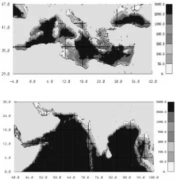
In this work, WAM is used in two different wave-climate re-gions: the Mediterranean Sea, a wind sea dominated area, and the Indian Ocean, a swell dominated one. The two model domains are illustrated in Fig. 1. A global version of the model is used in order to initialize and nudge the lat-eral boundaries of the Indian Ocean domain. All the versions ran on high resolution set up, in a deep water mode without refraction, providing operationally daily forecasts.
For the integration in the global domain, 28 frequencies and 24 directions were used, while the first integration fre-quency was 0.05 Hz and the propagation time step 1200 s. The same configuration holds for the nested domain of the Indian Ocean, with a propagation time step of 600 s. On the other hand, for the Mediterranean Sea, taking into account the shorter scale of the prevailing atmospheric and wave sys-tems, the number of frequencies was limited to 25 and the first one was set to 0.1 Hz. The time step in this case was 300 s.
Different atmospheric inputs (wind speed and direction 10 m above surface) were used for the above domains. The global model is driven by wind fields of the NCEP/GFS model that has a horizontal grid resolution 1.0×1.0 degrees. The nested Indian Ocean as well as the Mediterranean Sea use SKIRON/ETA weather prediction system (Kallos, 1997; Papadopoulos et al., 2001) which runs operationally once a day (with 12:00 UTC initial conditions) at the University of Athens, providing 5-day forecasts2. This system uses NCEP/GFS 1.0×1.0 degree resolution fields for the initial and boundary conditions. The necessary surface boundary conditions over the sea are interpolated from the 0.5×0.5 de-gree SST (Sea Surface Temperature) field analysis retrieved from NCEP on a daily basis. Vegetation and topography data are applied at a resolution of 30 s and soil texture data with resolution of 2 min. Further details of the models’ configura-tion are summarized in the Table 1.
Both the atmospheric and wave models use the same high resolution in order to avoid interpolation issues and to ensure a better description of short scale atmospheric and wave
phe-2http://forecast.mg.uoa.gr
Figure 3.1. Mediterranean Sea and Indian Ocean bathymetry (m).
Fig. 1. Mediterranean Sea and Indian Ocean bathymetry (m).
nomena (e.g. local coastal atmospheric circulations, island wave effects, etc.).
The assimilation scheme described in Sect. 2 was applied to both areas of interest. The number of iterations used was k=5 (as defined in Sect. 2) and the de-correlation radius b (grid distances) was defined to be 4. The maximum influence radius of assimilation was 8 grid points (this is only a prac-tical limit, set when the correlation following this expression is close to zero). The maximum influence and decorrelation radius are compatible with the wave model resolution, since they are defined as grid point distances. In our case, these parameters are chosen so as to reflect the scales of the atmo-spheric forcing wind field at the sea surface and to be rep-resentative of the wave system characteristics prevailing and influencing each area. More precisely, according to the above definitions, for the Mediterranean Sea the decorrelation ra-dius was 40 km and the maximum influence rara-dius 80 km,
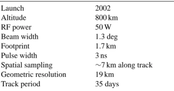
Table 2. ENVISAT technical characteristics.
Launch 2002
Altitude 800 km RF power 50 W Beam width 1.3 deg Footprint 1.7 km Pulse width 3 ns
Spatial sampling ∼7 km along track Geometric resolution 19 km
Track period 35 days
where in the Indian Ocean they were 100 and 200 km, re-spectively. The standard deviation of the model was set to Ep=1.0 m and the observation error to E0=0.5 m. These
val-ues were set based on the assumption that synoptic wind sys-tems and the generated wave ones are of similar scale. This assumption is required due to the operational status of the present study.
Observations from the Ku-band of ENVISAT-ESA Radar
Altimeter 2 (RA-2) were used in the assimilation cycle. This
instrument determines the two-way delay of the radar echo from the Earth’s surface to a very high precision (less than a nanosecond) with a footprint size of 1.7 km. In this way, the determination of wind speed and significant wave height is achieved. In particular, the significant wave height is cal-culated from the radar echo leading edge slope, which refers to the gradient of the leading edge of the echo. According to previous studies, the expected accuracy for the measure-ment of wave height is better than 0.25 m (see ESA SP-1224; Soussi, 2006). Some basic technical characteristics of this platform are presented in Table 2.
In both areas of interest the altimeter data were quality controlled according to Brattli (2003). More precisely, the basic filtering criteria used were the following:
– Significant wave height observations should be between
0.5 and 20 m.
– Altimeter data standard deviation should not exceed a
given interval (0.01–1 m).
– The difference between the model first guess and the
RA2 record must be less than 5 m.
The restricted standard deviation interval (second criterion) ensures that extremely variable measurements will be ex-cluded. The remaining variability of the altimeter data is desirable and necessary in order to better exploit the high resolution simulations.
For the Mediterranean Sea the average number of assim-ilated observations per forecasting cycle, passing this qual-ity control, was between 250 and 300. The corresponding number for the Indian Ocean was 550–650. It is obvious that such an amount of “information” in open seas or oceans,
where other types of observations are rare, is a valuable tool. The assimilation window in both areas was determined to be 12 h. More precisely, all observations available between 12:00–24:00 UTC are used. Note that the assimilation of these records is not taking place at a specific time. Since our system is running operationally, the assimilation procedure is active during the whole 12-h window, so that every recorded observation is assimilated at the closest model time step. In this way, corrected fields at 00:00 UTC are obtained which are used as analysis for the forecasting period from 00:00 to 12:00 UTC of the next day.
4 Results
The wave forecasting systems, described in the previous section, ran for a period of two months during November– December 2004 for the Indian Ocean and December 2004– February 2005 for the Mediterranean Sea. Some separate test cases were also performed in order to study the impact of the assimilation scheme under different weather conditions and will be described in the following. The first five days were used so as to reach a well established sea state.
The statistical analysis used in the present work was based on the following parameters:
– Mean Difference and Root Mean Square Error of the
Difference (RMSE) calculated between WAM, with and without assimilation,
– Mean Difference, RMSE, Correlation Coefficient and
Standard Deviation between the two versions of WAM (with and without assimilation) and satellite (RA2) measurements.
In this way, the quantitative impact of the assimilation in wave forecasts, as well as the quality of the analyzed wave fields, are estimated. The same statistical parameters were also employed for model evaluation against buoy observa-tions.
Before proceeding with the discussion of the results, it is important to undeline that the two domains selected (the Mediterranean Sea and the Indian Ocean) are characterized by different physiographic characteristics, synoptic weather conditions and wave climatology. The long period waves (swell) are the dominant mode of the sea state in the In-dian Ocean, since it can receive waves that have travelled even from Antarctica. On the other hand, in the Mediter-ranean Sea, wind-generated waves are significant and the wind regime in winter is more unstable. These facts are il-lustrated in Fig. 2, where the swell percentage of the total sea state, as well as the mean wave (spectral) period at each grid point for the experiment time, is presented. It becomes ob-vious that the maximum simulated mean wave period in the Mediterranean Sea is less than 6 s while this value is the min-imum one for the Indian Ocean, where a typical wave period
(a)
(b)
Figure 4.1. Mean wave period in seconds (a) and Swell percentage (b) of total
Fig. 2. Mean wave period in seconds (a) and swell percentage (b) of total wave energy.
MEDITERRANEAN SEA INDIAN OCEAN
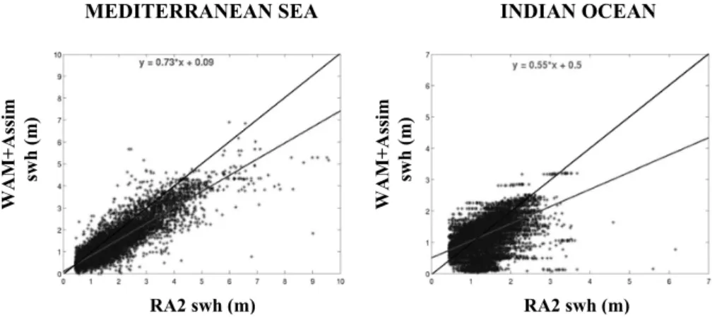
Figure 4.2. Linear correlation between wave model (no data assimilation) and
WA M s w h (m ) WA M s w h (m ) RA2 swh (m) RA2 swh (m)
Fig. 3. Linear correlation between wave model (no data assimilation) and satellite significant wave height over all forecasting hours.
fluctuates between 7–10 s. This difference between the two areas is further supported by the fact that the swell percent-age in the Indian Ocean exceeds 80%, reaching in several cases even 100% of the total wave energy, whereas in the Mediterranean it is always less than 80%.
However, it has to be noted that during the boreal winter, for a large portion of the time, relatively steady northeast-erly winds are prevailing in the northern Indian Ocean. This generates well developed windsea, which is more evident at the eastern coast of India. The model interprets such situa-tions as swell. This fact creates problems in the identification
of young windsea when swell is present (see Janssen et al., 2005; Bidlot et al., 2007) contributing also in the state repre-sented at Fig. 2.
These different characteristics in the two domains, along with the fact that the assimilation analysis does not correct the wind input from the atmospheric model but directly the significant wave height, favors a limited influence of the as-similation scheme in the Mediterranean Sea (see also Li-onello et al., 1992).
Concerning the initial relation between satellite data and the wave model with no data assimilation, it is worth noticing
MEDITERRANEAN SEA INDIAN OCEAN
Figure 4.3. Linear correlation between wave model with assimilation (correcte
WA M + A ss im sw h (m ) RA2 swh (m) RA2 swh (m) WA M + A ss im sw h (m )
Fig. 4. Linear correlation between wave model with assimilation (corrected forecasts) and satellite significant wave height over all forecasting
hours. 0.5 0.55 0.6 0.65 0.7 0.75 0.8 0.85 0.9 0.95 1 4 7 10 13 16 19 22 25 28 31 34 37 40 43 46 49 52 55 58 61 Integration Time (h) S ig n W a v e H e ig h t (m ) WH assim WH noassim
Fig. 5. Significant wave height time series for one assimilated
ob-servation in the Mediterranean Sea (WAM direct output = 0.7 m, Observation = 0.9 m).
that it differs significantly in the two areas of interest. In particular, in the Mediterranean Sea, the corresponding lin-ear correlation is significantly higher than that of the Indian Ocean. However, significant wave height is strongly under-estimated at high values in the first area (Fig. 3). This is a reason that potentially may limit the impact of the assimila-tion scheme in the first domain. Indeed, the corresponding results for the wave model with the assimilation module ac-tivated show a trivial influence in the Mediterranean area (cf. Table 3).
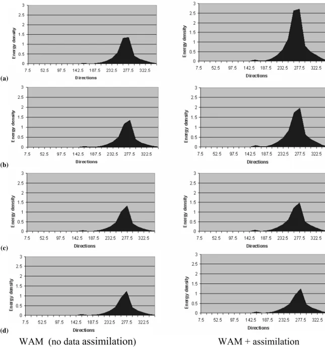
Focusing now on the results of the assimilation, the way that it modifies the model energy spectrum is investigated. For this reason, several cases of single-observation inputs in WAM were studied. The corresponding results were almost identical in all tests and a typical case is presented here as an example. More specifically, a grid point was selected where the WAM first-guess was 0.7 m, whereas the analyzed wave height was estimated to 0.9 m. In this case, the directional and the frequency energy distribution remained unchanged after the data assimilation, increasing, however, the total en-ergy amount (Figs. 6–8). This was an expected outcome,
since only significant wave height is assimilated and there-fore no other directional or frequencial information is avail-able. The assimilation impact lasted almost 6 h, as clearly indicated in Figs. 5–7. However, this period becomes longer for higher differences between model outputs and satellite records while the general attribute remains similar.
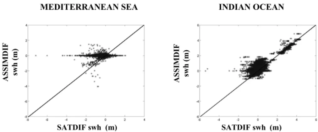
In the sequel, an assimilation impact factor is derived by comparing the deviations between the results of WAM with the data assimilation and the reference run – no assimilation – denoted as ASSIMDIF (y-axis), to the deviations between satellite measurements and the model with no data assimila-tion – SATDIF (x-axis), as shown in Fig. 9. The large number of low values for ASSIMDIF in the first plot (Mediterranean) is partly due to the previous mentioned high correlation be-tween satellite measurements and the model’s results without data assimilation. Moreover, some extreme differences be-tween satellite data and model outputs seem to be smoothed by the assimilation. On the contrary, in the area of the In-dian Ocean, the adjustment of the values to the diagonal line indicates that the activation of the assimilation module re-duces the initial differences emerging between observations and forecasted results.
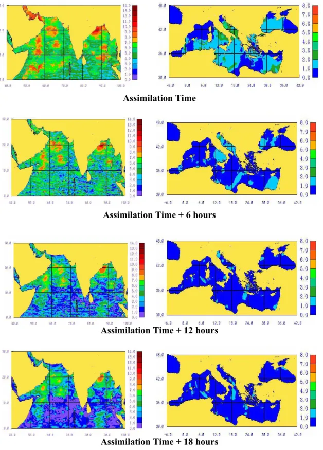
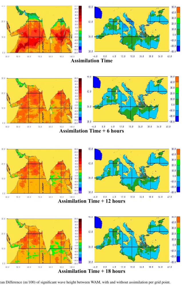
A detailed study concerning the assimilation impact at each model grid point, as well as its evolution in time fol-lows. More precisely, in Figs. 10 and 11, the average RMSE and mean difference between the results of the two models (with and without the assimilation) for the whole testing pe-riod and for different forecasting hours are presented. Con-cerning the time evolution of assimilation impact, the maxi-mum deviations seem to emerge at 18:00 UTC in the Indian Ocean and at 00:00 UTC in the Mediterranean (“assimila-tion time” for each domain, respectively), due to the different time that satellite tracks pass over these areas. This influence in the Mediterranean Sea is reduced after a period of less than 12 h, while in the Indian Ocean it remains significant for the whole forecasting period as a result of the “longer memory” of swell waves. Moreover, this impact seems to be translated
(a)
a.
b.
(b)b.
(c)c.
d.
(d)d.
WAM (no data assimilation) WAM + assimilation
WAM (no data assimilation) WAM + assimilation
Figure 4.5.
Frequency (Hz) - Energy density (m
2) diagrams for different times after
Fig. 6. Frequency (Hz)-Energy density (m2) diagrams for different times after the assimilation: (a) analysis time, (b) 2-h-forecast, (c) 4-h-forecast, (d) 6-h-forecast.
Table 3. Statistical evaluation of the two versions of WAM (no data assimilation and corrected forecasts) vs. RA 2 measurements for the
whole study period.
Mean difference St. Deviation Cor. Coefficient Medit. Indian Medit. Indian Medit. Indian RA2 – Model (no data
assimila-tion)
−0.37 0.12 0.49 0.67 0.88 0.20∗
RA2 – Model (corrected forecast) −0.39 −0.11 0.49 0.43 0.88 0.53
∗
(a)
a.
b.
(b)b.
(c)c.
d.
(d)d.
WAM (no data
assimilation
) WAM + assimilation
WAM (no data assimilation) WAM + assimilation
Figure 4.6.
Direction (deg) - Energy density (m
2) diagrams for different times after
Fig. 7. Direction (degrees)-Energy density (m2) diagrams for different times after the assimilation: (a) analysis time, (b) 2-h-forecast, (c) 4-h-forecast, (d) 6-h-forecast.
to northern latitudes due to the usually prevailing southerly waves.
On the other hand, it is clear that in the Mediterranean Sea the assimilation influence is quite local, while the whole Indian Ocean domain is affected. Additionally, the max-imum values of both statistical parameters used are lower in the Mediterranean (RMSE<0.3 m, −0.2 m < Mean Dif-ference <0.1 m) compared to those of the Indian Ocean (RMSE<1.4 m, 0 m < Mean Difference <1.0 m). This is mainly due to the local characteristics of the Mediterranean
basin: closed sea with well separated sections where a pos-sible correction in one area remains restricted there and does not propagate. On the contrary, the fact that the Indian Ocean is swell-dominated, as well as the increased initial differ-ences between RA2-altimeter and model results without as-similation, led to an extended impact in this area. At the same time, a number of extreme differences which emerged between the model without assimilation and satellite records in the Indian Ocean (as shown in Fig. 3) were reduced and the corresponding coefficient of the linear regression line was
Figure 4.7.
Fig. 8. Energy spectrum distribution (polar diagrams) at the assimilation time.Energy spectrum distribution (polar diagrams) at the assimilation tim
MEDITERRANEAN SEA INDIAN OCEAN
SATDIF swh (m) SATDIF swh (m) A S S IM D IF sw h (m ) A S S IM D IF sw h (m )
Fig. 9. Deviations of assimilated results and satellite data against predictions. ASSIMDIF (y-axis) denotes the difference between the results
of WAM, with and without assimilation, while SATDIF (x-axis) stands for the deviations between satellite measurements and model results.
almost doubled (Fig. 4). These differences were due to a 3-day failure in the atmospheric and wave forecasting as a re-sult of a misplaced forecasted storm. However, the use of the assimilation scheme reduced these differences, thus leading to the conclusion that the data assimilation has made up for the shortcomings in the wave model results.
Focusing now on the average statistical results concerning the entire domain of each case, Table 3 illustrates that altime-ter data assimilation procedure had no obvious impact in the Mediterranean Sea. Note that the statistical parameters used refer to RA2 observations against the closest WAM grid point at the assimilation time. On the contrary, in the Indian Ocean,
the initially observed differences between satellite measure-ments and model outputs were reduced and their correlation becomes remarkably higher. It is also worth noticing that the low initial correlation between RA2 measurements and WAM outputs in the Indian Ocean is partly due to the short period of model failure which was referred earlier.
In order to further evaluate the wave model forecasts, a de-tailed comparison against available buoys is presented. For the Mediterranean Sea, the buoy data have been provided by the Spanish Puertos del Estado (P.E.) and the Hellenic Cen-ter for Marine Research (HCMR). Their location is shown in Figs. 12, 13 and Table 4. These data were processed and
Assimilation Time
Assimilation Time + 6 hours
Assimilation Time + 12 hours
Assimilation Time + 18 hours
Figure 4.9.
Assimilation Time
Assimilation Time + 6 hours
Assimilation Time + 12 hours
Assimilation Time + 18 hours
Figure 4.10.
Mean Difference (m/100) of significant wave height between WAM
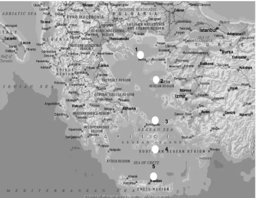
1 2 3 4 5
Fig. 12. Aegean Sea buoy locations.
Figure 4.12. Spanish buoy locations.
6
7
Fig. 13. Spanish buoy locations.
quality controlled by the providing institutes. Each buoy was collocated with the closest model grid point and the corre-sponding significant wave height values were compared in
3-h intervals. In both cases (Spain and Greece) the neg-ligible effect of the assimilation procedure in the Mediter-ranean Sea is reconfirmed. This is mainly due to the fact
Alicante 0.6 0.7 0.8 0.9 1 1.1 1.2 1.3 1.4 1.5 1.6 2004120300 2004120400 2004120500 Date Sw h (m ) buoy noassim assim Athos 0 0.5 1 1.5 2 2.5 3 3.5 4 4.5 5 2004120300 2004120500 2004120700 2004120900 Date Sw h (m ) buoy noassim assim Avgo 0 0.2 0.4 0.6 0.8 1 1.2 1.4 1.6 1.8 2 2004120300 2004120400 2004120500 2004120600 Date Sw h (m ) buoy noassim assim
Figure 14. Time series of significant wave height of buoy, WFig. 14. Time series of significant wave height of buoy, WAM and
WAM + assimilation.
Table 4. Mediterranean buoy coordinates.
Buoy Latitude Longitude 1. Athos 40.0 24.7 2. Lesvos 39.2 25.8 3. Mikonos 37.5 25.5 4. Santorini 36.3 25.5 5. Avgo 36.0 25.6 6. Alicante 38.2 −0.4 7. Gata 36.6 −2.3 DS 1 DS 3
Fig. 15. Indian Ocean buoy locations.
Table 5. Indian buoy coordinates.
Buoy Latitude Longitude DS1 15.60 69.19 DS3 12.15 90.74
that the number of satellite measurements passing the assim-ilation quality control is limited for areas close to coasts or islands, as in the Aegean Sea. However, whenever sufficient altimeter measurements are available, the benefit from the assimilation impact is clear, although temporary (as shown in Fig. 14), significantly improving the underestimated – in general – WAM forecasts.
For the domain of the Indian Ocean, two buoys have been employed, as provided by the National Institute of Ocean and Technology (NIOT) of India. Their position and geographic coordinates are illustrated in Fig. 15 and Table 5, respec-tively. The comparison between the two versions of WAM (with and without assimilation) and these buoys show a clear improvement in the performance of the model. More pre-cisely, the mean error of the results is reduced significantly by the use of altimeter data. The relatively low correlation coefficient may be attributed to the small significant wave heights dominating during the analysis period. The corre-sponding time-series, along with statistical results are pre-sented in Fig. 16.
5 Conclusions
The performance of a data assimilation scheme using altimeter-RA2 records in high resolution versions of the WAM model has been tested in two different wave climate regions: the Mediterranean Sea and the Indian Ocean. The local characteristics of these domains affect the quality as well as the amplitude of the assimilation impact. More precisely, the influence of the assimilation scheme in the Mediterranean Sea is limited mainly due to:
Buoy DS1 0,5 1 1,5 2 1 25 49 73 97 121 145 169 193 217 241 265 289 313 337 Forecasting period (h) Sw h ( m )
WAM No Assim WAM + Assim RA2 Buoy
Buoy DS1 NoAssim vs Buoy AssimRA2 vs Buoy Mean Difference 0.50 0.39 RMSE 0.60 0.45 Cor.Coef. 0.25 0.43 Buoy DS3 0,6 0,8 1 1,2 1,4 1,6 1,8 2 1 25 49 73 97 121 Forecasting period (h) Sw h ( m )
WAM No Assim WAM + Assim RA2 Buoy
Buoy DS3 NoAssim vs Buoy AssimRA2 vs Buoy Mean Difference 0.44 0.15 RMSE 1.14 0.30 Cor.Coef. 0.46 0.57
Fig. 16. Time series and statistical results of significant wave height for buoys, WAM and WAM + assimilation.
– the lack of a sufficient number of observation data. This
is a result of the fact that satellite measurements in coastal areas are usually of low quality and, therefore, fail to pass the quality controls,
– the fact that the assimilation analysis scheme does not
correct the wind input from the atmospheric model but directly the forecasted significant wave height. This is a disadvantage of the method in wind-sea dominated ar-eas, like the Mediterranean Sea,
– the local characteristics of the Mediterranean basin: it is
a closed sea with complicated coast line, several islands and well separated sections where a possible (assimila-tion) impact in one area remains restricted and dimin-ishes there,
– the high correlation of the filtered satellite records with
model first guess.
However, the final forecasting quality of the wave system (WAM+assimilation module) is at a very satisfactory level.
On the other hand, for the Indian Ocean, the large num-ber of available satellite observations, combined with the fact
that this is a swell dominated area, leads to an increased as-similation impact extended to the entire domain. In particu-lar, the assimilation of altimeter data leads to:
– the reduction of model error,
– the elimination of any possible significant differences
between the WAM first guess and satellite records. Acknowledgements. This work is supported by the EU-funded
project EnviWave (EVG-2001-00017). SINTEF and DNMI are ac-knowledged for the cooperation during this project concerning data filtering and assimilation algorithms.
Topical Editor S. Gulev thanks two referees for their help in evaluating this paper.
References
Aarnes, J. E.: Iterative methods for data assimilation and an appli-cation to ocean state modeling, SINTEF Applied Mathematics, 2003.
Abdalla, S., Bidlot, J., and Janssen, P.: Assimilation of ERS and ENVISAT wave data at ECMWF, Proceedings of the 2004 EN-VISAT & ERS Symposium, Salzburg, Austria, 6–10 September 2004; ESA SP-572, April 2005.
Bidlot, J.-R., Janssen, P., and Abdalla, S.: Impact of the revised formulation for ocean wave dissipation on ECMWF operational wave model, ECMWF Tech. Memo., 509, ECMWF, Reading, UK, 2007.
Brattli, A. and Breivik, L. A.: Geophysical Evaluation of ENVISAT RA-2 Data, Norwegian Met. Institute, Report No. 147, 2003. Breivik, L. A. and Reistad, M.: Assimilation of ERS-1
Altime-ter Wave Heights in an Operational Numerical Wave Model, Weather and Forecasting, 9(3), 440–451, 1994.
Bouttier, F. and Courtier, P.: Data assimilation concepts and meth-ods, Meteorological Training Course Lecture Series, ECMWF, 1999.
Bratseth, A.: Statistical interpolation by means of successive cor-rections, Tellus Ser.A, 38, 439–447, 1986.
Cressman, G. P.: An Operational Objective Analysis System. Mon. Wea. Rev., 87, 367–374, 1959.
ESA SP-1224, EnviSat: The Altimetry Report, Science and Appli-cations, 1999.
Greenslade, D.: The assimilation of ERS-2 significant wave height data in the Australian region, J. Mar. Syst., 28, 141–160, 2001. Janssen, P. A. E. M., Lionello, P., Reistad, M., and Hollingsworth,
A.: A study of the feasibility of using sea and wind information from the ERS-1 satellite, part 2: Use of scatterometer and altime-ter data in wave modelling and assimilation, ECMWF report to ESA, Reading, 1987.
Janssen, P., Bidlot, J.-R., Abdalla, S., and Hersbach, H.: Progress in ocean wave forecasting at ECMWF, ECMWF Tech Memo, 478, ECMWF, Reading, United Kingdom, 2005.
Kallos, G., Nickovic, S., Sakellaridis, G., et al.: The Regional weather forecasting system SKIRON, Proceedings, Symposium on Regional Weather Prediction on Parallel Computer Environ-ments, Athens, Greece, 1997.
Komen, G. J., Cavaleri, L., Donelan, M., Hasselmann, K., Hassel-mann, S., and Janssen, P. A. E. M.: Dynamics and Modelling of ocean waves, Cambridge University Press, 1994.
Lionello, P., G¨unther, H., and Hansen, B.: A sequential assimilation scheme applied to global wave analysis and prediction, J. Mar. Syst., 6, 87–107, 1995.
Lionello, P., G¨unther, H., and Janssen, P. A. E. M.: Assimilation of altimeter data in a global third generation wave model, J. Geo-phys. Res., 97(C9), 14 453–14 474, 1992.
Papadopoulos, A., Katsafados, P., and Kallos, G.: Regional weather forecasting for marine application, Global Atmos. Ocean Syst., 8(2–3), 219–237, 2001.
Skandrani, C., Lef`evre, J. M., and Queffeulou, P.: Impact of Mul-tisatellite Altimeter Data Assimilation on Wave Analysis and Forecast, Marine Geodesy, 27, 1–23, 2004.
Soussi, B.: ENVISAT RA-2/MWR Level 2 User Manual, Issue Number 1.2, 20 June 2006.
WAMDIG, The WAM-Development and Implementation Group: Hasselmann, S., Hasselmann, K., Bauer, E., Bertotti, L., Car-done, C. V., Ewing, J. A., Greenwood, J. A., Guillaume, A., Janssen, P. A. E. M., Komen, G. J., Lionello, P., Reistad, M., and Zambresky, L.: The WAM Model – a third generation ocean wave prediction model, J. Phys. Oceanogr., 18(12), 1775–1810, 1988.