Nautilus multi-grain model: Importance of cosmic-ray-induced desorption in determining the chemical abundances in the ISM

(1)

HAL Id: hal-01725052

https://hal.archives-ouvertes.fr/hal-01725052

Submitted on 11 Nov 2020

HAL is a multi-disciplinary open access

archive for the deposit and dissemination of

sci-entific research documents, whether they are

pub-lished or not. The documents may come from

teaching and research institutions in France or

abroad, or from public or private research centers.

L’archive ouverte pluridisciplinaire HAL, est

destinée au dépôt et à la diffusion de documents

scientifiques de niveau recherche, publiés ou non,

émanant des établissements d’enseignement et de

recherche français ou étrangers, des laboratoires

publics ou privés.

Nautilus multi-grain model: Importance of

cosmic-ray-induced desorption in determining the

chemical abundances in the ISM

Wasim Iqbal, Valentine Wakelam

To cite this version:

Wasim Iqbal, Valentine Wakelam. Nautilus multi-grain model: Importance of cosmic-ray-induced

desorption in determining the chemical abundances in the ISM. Astronomy and Astrophysics - A&A,

EDP Sciences, 2018, 615, pp.A20. �10.1051/0004-6361/201732486�. �hal-01725052�

(2)

Astronomy

_&

Astrophysics

https://doi.org/10.1051/0004-6361/201732486

Nautilus multi-grain model: Importance of cosmic-ray-induced

desorption in determining the chemical abundances in the ISM

Wasim Iqbal and Valentine Wakelam

Laboratoire d’astrophysique de Bordeaux, Univ. Bordeaux, CNRS, B18N, allée Geoffroy Saint-Hilaire, 33615 Pessac, France e-mail: wasimiqbal2009@gmail.com; valentine.wakelam@u-bordeaux.fr

Received 18 December 2017 / Accepted 12 February 2018

ABSTRACT

Context. Species abundances in the interstellar medium (ISM) strongly depend on the chemistry occurring at the surfaces of the dust grains. To describe the complexity of the chemistry, various numerical models have been constructed. In most of these models, the grains are described by a single size of 0.1 µm.

Aims. We study the impact on the abundances of many species observed in the cold cores by considering several grain sizes in the Nautilus multi-grain model.

Methods. We used grain sizes with radii in the range of 0.005 µm to 0.25 µm. We sampled this range in many bins. We used the previously published, MRN and WD grain size distributions to calculate the number density of grains in each bin. Other parameters such as the grain surface temperature or the cosmic-ray-induced desorption rates also vary with grain sizes.

Results. We present the abundances of various molecules in the gas phase and also on the dust surface at different time intervals during the simulation. We present a comparative study of results obtained using the single grain and the multi-grain models. We also compare our results with the observed abundances in TMC-1 and L134N clouds.

Conclusions. We show that the grain size, the grain size dependent surface temperature and the peak surface temperature induced by cosmic ray collisions, play key roles in determining the ice and the gas phase abundances of various molecules. We also show that the differences between the MRN and the WD models are crucial for better fitting the observed abundances in different regions in the ISM. We show that the small grains play a very important role in the enrichment of the gas phase with the species which are mainly formed on the grain surface, as non-thermal desorption induced by collisions of cosmic ray particles is very efficient on the small grains.

Key words. astrochemistry – ISM: molecules – ISM: clouds – ISM: abundances – molecular processes – cosmic rays

1. Introduction

The interstellar medium (ISM) is rich in many molecular and atomic species either in the positively or the negatively charged states or in the neutral form. The ISM is also filled with different types of radiation fields such as UV photons (called interstel-lar radiation field) and cosmic rays. The local physical and irradiation conditions determine the main physio-chemical pro-cesses governing the chemical composition of the interstellar matter. In this context, the interstellar dust grains are of partic-ular importance as they act as the surfaces where the gaseous species (atomic or molecular) can stick, diffuse, and react with each other to form new species. Numerical models based on the rate equation approximation are the most popular tool for studying the gas-grain chemistry and to simulate the evolution of complex chemical species with time, due to their very rapid execution (Wakelam et al. 2013). In general, as a simplification, these models consider a single grain size with radius 0.1 µm as a representative of all interstellar grains, which essentially results in all grains having the same physical and chemical properties

(Hasegawa et al. 1992; Hasegawa & Herbst 1993b and more

recentlyGarrod 2008;Wakelam & Herbst 2008;Wakelam et al.

2010; Ruaud et al. 2016). This assumption greatly reduces the

difficulties in implementation of rate equations and also saves on computing time. There are a few published studies where the authors studied the impact of this assumption by considering several grain sizes in their model. Acharyya et al.(2011), for

instance, assumed five different grain sizes but the dust tem-perature was kept constant for all grain sizes. The conclusion of his work was that gas phase abundance of any species form-ing on the surface of dust grains depends on the effective total surface area of dust grains and this can also be achieved by using a single-grain model and proper number density of grains so that the total surface area remains constant. Following this work, Pauly & Garrod (2016) andGe et al. (2016) developed models in which they used grains of different sizes. There were however two limitations to these works: They used a small number of grain sizes, and did not, as far as we know, con-sider the effect of cosmic-ray induced desorption as a function of grain radius, which strongly depends on the grain size. As

Herbst & Cuppen (2006) showed, the surface temperature of

very small grains (radius ≈ 0.005 µm) can rise above 300 K, whereas that of big 0.25 µm grains only reaches about 50 K. This can result in significant desorption of species from the sur-face of small grains while big grains can remain very much unaffected.

In this work, we have revisited the effect of considering sev-eral grain sizes in our gas-grain model Nautilus in the conditions of cold cores, where the cosmic ray induced desorption can play an important role. While changing the size of the grains, several processes and model parameters are changed, such as the num-ber density of each grain population, the surface temperature, and the peak surface temperature due to cosmic ray collisions with dust grains, among others.

A20, page 1 of16

(3)

A&A 615, A20 (2018) The paper is organized as follows. In Sect. 2, we present

the Nautilus gas-grain model and the modifications made to include the different grain sizes. In Sect.3, we present our results obtained using the multi-grain model and also compare these results with the single-grain Nautilus model. In Sect.4, we com-pare our results with observations in TMC-1 and L134N clouds, and in Sect.5, we discuss the effect of scaling the cosmic ray peak duration on small grains. Some conclusions are given in the last section.

2. Nautilus gas-grain code

The Nautilus gas-grain code uses rate equation approximation

(Hasegawa et al. 1992;Hasegawa & Herbst 1993b) to simulate

the chemical evolution in the ISM. The latest version of this code is based on the three-phase model fromRuaud et al.(2016). It simulates the chemical evolution in the gas, on the grain surface, and within the grain mantle with all three phases coupled to each other. The gas-phase chemistry is based on the kida.uva.2014 public network (Wakelam et al. 2015) while the surface chem-istry is the same as in Ruaud et al. (2016). In addition to the gas-phase chemistry, the model includes the physisorption of neutral species on the surface of grains, the diffusion of these species, and their reactions. Desorption of species can only occur from the surface (not the mantle) but the surface is of course reconstructed by the mantle species as the surface species evapo-rate. Similarly, as species are accreted on the surface, the species from the surface are incorporated to the mantle. In addition to thermal desorption, we consider nonthermal desorption pro-cesses such as cosmic-ray-induced desorption, UV (direct and indirect) photo-desorption, and chemical desorption. All details of the model are described inRuaud et al.(2016).

2.1. Implementation of multi-grain network and grain size distribution

In the original version, grains are considered to have a single size of 0.1 µm and a silicate composition (Hasegawa et al. 1992). Using 0.1 µm as the grain radius, assuming a gas to dust mass ratio of 102 and a dust bulk density of 3 g cm−3, we obtain a grain number density of 1.8 × 10−12_n

H, where nHis the number

density of H (in cm−3). If there are 106binding sites on the sur-face of a 0.1 µm grain (seeHasegawa et al. 1992), we then obtain a surface site density of 8 × 1014_cm−2_{. These values are the ones}

usually used in chemical models and also in our “single grain size” model.

The aim of this work is to include several sizes of grains in Nautilus to obtain a more realistic description of the ISM conditions. This modified version of Nautilus is called Nautilus Multi Grain Code (NMGC). To obtain the different grain sizes, we have sampled the total range between the smallest and the biggest grains (0.005 µm and 0.25 µm, respectively) in our sim-ulation in either 10, 30, or 60 bins. These numbers are arbitrary and one can use any desired number of grain sizes in the sim-ulations provided computational time permits. For example, on a laptop with Intel®Xeon® E3-1505M v5 CPU @ 2.80GHz, a simulation with ten grain sizes or bins takes about 2 min to reach 107 yr but with 60 grain sizes, to reach this point takes about 30 min.

In NMGC, all grains are connected with each other through a common gas phase. Two grains never interact directly or exchange mass or energy directly with each other. In other words there is no collision of dust grains. Exchange of mass is only possible through the process of desorption of the surface species

to the gas phase and the accretion of gaseous species on the dust surface. However, one side effect of the rate equations method is that all species on the grains of the same size can interact with each other (as was the case for the single grain size model also) but there is no interaction between surface molecules on grains of different sizes. In our multi-grain model, the chemical net-works on the surface of grains have been duplicated for different bins by adding a number as prefix to each grain species. This number is specific to each bin. Some or all major properties of each grain size in the multi-grain network can be varied indepen-dently to meet the specific requirement of various environments. The most important properties of a grain in regards to model-ing a chemical evolution are the radius and correspondmodel-ing grain number density, the surface temperature, and the grain composi-tion. To compute the number densities of each grain bin, we used two grain size distribution models. The first model is the MRN distribution from Mathis et al.(1977). The MRN model gives the number density of grains with radii between r and r+ dr by the expression: 1 nH dngr dr = Cr −3.5_{; r} min< r < rmax, (1)

where ngr is the grain number density, r is grain radius, nH is

H number density and C is called grain constant. C is given by 10−25.11_cm2.5 _{for silicate grains and 10}−25.13_cm2.5 _{for graphite}

grains (Weingartner & Draine 2001). The above relation is valid between rmin = 0.005 µm and rmax = 0.25 µm. The

second model we used is widely called the WD model from

Weingartner & Draine(2001). The WD model relies on many

parameters that are specific to different regions of the ISM. Fol-lowingAcharyya et al.(2011), we selected Rv= 5.5, case A, and bc = 3 × 105. These parameters are suitable for dense clouds.

The total grain surface available for accretion of the species directly depends on the number density of grains. The total effec-tive surface area depends on our choice of sampling (number of bins) as well as on the grain size distribution model. In previous works,Acharyya et al. (2011) used only five different sizes of grains in their multi-grain model,Pauly & Garrod(2016) used between five and eleven bins, and Ge et al. (2016) used nine different bins.Iqbal et al.(2014) showed that if the number of dif-ferent grain sizes is less than 30, then the total integrated grain density is significantly smaller as compared to the total grain density predicted by the grain size distribution models. In this work, we have considered 1, 10, 30, and 60 grain sizes, and stud-ied the impact of this choice on the chemistry. Another advantage of using a better sampling is that we obtain a better estimate of each grain family temperature as a function of size.

The MRN model is valid between rmin = 0.005 µm and

rmax= 0.25 µm. We used the same interval for both the MRN and

WD models for a better comparison of the results. We divided the range (0.005 µm to 0.25 µm) into 10, 30 and 60 logarith-mically equally spaced points, which gives us a value for the radius ri. We use this rivalue to calculate the surface area and

other surface parameters for the corresponding range defined by rmin= (r(i−1)+ ri)/2 and rmax = (r(i₊₁₎+ ri)/2, except for the first

bin in which rmin = riand last bin in which rmax= ri. Then we

calculate the grain number density ngr(i) for both models, with local rmin(i) and rmax(i) values. We plot the grain radius against

bin width in Fig.1. The height of each rectangular column repre-sents the grain radius riand the width of each rectangular column

represents the bin width or rmax(i) − rmin(i). In Fig.2, we plot the

integrated grain number density or grain abundance as a function of ri(bottom panel) and the effective surface area (ngr(i)× 4πr_i2)

(4)

Fig. 1.Bin width as a function of grain radius. The width of each vertical column represents bin width and the height of each vertical column represents the radius of the representative grain in that bin. Since we divide the entire range on log scale with equal spacing, in linear scale the width of each bin is different and increases with radius except for the last bin.

Table 1. Total effective grain surface area available for accretion (per cm3_{of space) in different models.}

Model Total effective surface area [cm2] Single grain size 2.26 × 10−21

MRN 10 grains 2.31 × 10−21 MRN 30 grains 2.36 × 10−21 MRN 60 grains 2.37 × 10−21 WD 10 grains 6.10 × 10−22 WD 30 grains 6.32 × 10−22 WD 60 grains 6.37 × 10−22

In Table1, we show the total effective surface areas in cm2

(available for accretion per cm3 of space) as calculated using different grain size distribution models. It is to be remembered that the total effective surface area depends on the bin size as well as on the radius used to represent that bin. We have tried to ensure that the total effective surface areas are close to each other in the same grain size distribution cases but with a dif-ferent number of bins. This is to minimize the possible effects on the accretion rates of different species caused by using dif-ferent numbers of bins. It can also be seen that some how the total effective surface areas calculated using the MRN models are very close to what we get in the single grain model in which the number density of grains is calculated by the dust to gas mass ratio only. The total effective surface area in the WD model is almost three and half time less than that in other models. This is because, in comparison to the MRN model, in the WD model small grains are less abundant and big grains are more abun-dant (see Fig. 2, bottom panel) and surface area decreases as we add small grains to make big grains, keeping the total mass constant.

2.2. Grain surface temperature and cosmic-ray-induced desorption

For the surface temperatures of different grain sizes, we assumed two different sets of models. First, we kept the grain temperature constant at 10 K for all grain sizes. As a second case, we used a different temperature for each bin or grain size. To derive this

temperature, we first compute the steady state dust temperature in diffuse medium conditions as a function of grain radius from

Draine & Lee (1984). Then we followed the recommendation

fromMathis et al.(1983) to multiply this value by 0.75 for dense cold medium. For our single-grain-size model, this method gives a dust temperature of 12 K. In our model we did not consider fluctuation in dust temperature due to UV or cosmic rays, but cosmic-ray-induced desorption is implemented in Nautilus code following the method described inHasegawa & Herbst(1993a). We modified our multi-grain model to account for different grain sizes. The cosmic-ray-induced desorption rate for any species on the ith grain is given by the equation:

kcrd(i) = f (Tmax(i))kevap(i, Tmax(i)), (2)

where f (Tmax(i)) is the duty cycle of the ith grain at elevated

temperature Tmax(i) and kevap(i, Tmax(i)) is the evaporation or

thermal desorption rate for the species on the ith grain at tem-perature Tmax(i). To estimate Tmax(i), we used the cosmic-ray

peak temperature as calculated by Herbst & Cuppen (2006) as a function of grain radius (assuming we have only silicate grains). f (Tmax(i)) is defined as the ratio of time-scale for cooling

via desorption of volatiles to the average time interval between two successive cosmic ray hits. FollowingHasegawa & Herbst

(1993a), for 0.1 µm grains, this interval is taken to be equal to 3.16 × 1013s, which comes from the Fe cosmic ray flux inLéger et al.(1985). We simply scaled it to obtain the flux for different grain sizes. At the densities of cold cores, cosmic rays are not completely attenuated (Umebayashi & Nakano 1981). The cos-mic rays deposit only a part of their energy into a grain during the interaction (see Eq. (4) ofHerbst & Cuppen 2006).

In previous models with single classical grains, the time-scale for cooling via desorption is taken to be 10−5s. This time is the half life of CO on the dust surface at 70 K. It is assumed that when a grain is heated to 70 K by collision with a cosmic-ray particle, CO is the most prominent species to desorb from the surface causing the grain cooling. It is also assumed that within this fraction of time, about 106 _{species would desorb from the}

surface, taking with them the extra energy deposited by cosmic rays and resulting in significant cooling of the grain. But when we are considering small grains of radii as small as 0.005 µm with a total number of sites equal to 2500 only, it is obvious that on small grains most of the time surface population would be

(5)

A&A 615, A20 (2018)

Fig. 2. Bottom panel: the grain abundance (with respect to the total proton density) in each bin plotted against the grain radius. Top panel: the total effective grain surface area (in cm2_{) of each bin for different}

models plotted against the grain radius. Legends apply to both panels.

only a fraction of 106_{. The cooling rates of small grains are then}

expected to be much slower and should result in lower surface population. In addition, this formalism of the cosmic ray desorp-tion assumes that there are CO molecules on the surface. In the absence of a better method to calculate or to scale this time for different grain sizes we used the same time period of 10−5_{s for}

all grain sizes in our multi-grain model. Considering the impor-tance of this assumption, further investigation in this process is needed.

The bottom panel of Fig.3 shows the grain radius for dif-ferent models and corresponding dust temperature, while the top panel shows the cosmic ray peak temperature as a function of grain radius.

Fig. 3.Bottom panel: grain temperature (circles for multi-grain model and star for single-grain model) as a function of grain radius. Top panel: peak surface temperature (triangles for multi-grain model and star for single-grain model) due to collision with cosmic rays as a function of grain radius.

Table 2. Elemental abundances and initial abundances. Element Abundance relative to H References

H2 0.5 He 0.09 a N 6.2 × 10−5 b O 2.4 × 10−4 c C+ 1.7 × 10−4 b S+ 8.0 × 10−9 d Si+ 8.0 × 10−9 d Fe+ 3.0 × 10−9 d Na+ 2.0 × 10−9 d Mg+ 7.0 × 10−9 d P+ 2.0 × 10−10 d Cl+ 1.0 × 10−9 d ice 0

References.(a)_{Wakelam & Herbst}₍₂₀₀₈_),(b)_Jenkins₍₂₀₀₉_),(c)_Hincelin et al.(2011),(d)_{Graedel et al.}₍₁₉₈₂_).

2.3. Other model parameters

We have run the different models using parameters for cold core conditions. In Table2, we have listed the elemental abun-dances and initial abunabun-dances used in our all models while Table3summarizes some important parameters which are kept

(6)

Table 3. Some important parameters used in our models.

Parameters Value

Tgas 10 K

nH 2 × 104cm−3

AV 15

Cosmic rays ionization rate 1.3 × 10−17_s−1

Grain surface site density 8.0 × 1014cm−2 Initial abundances see Table2

Fig. 4.Ice thickness as a function of grain radius for models with the MRN distribution and with the cosmic-ray-induced desorption enabled (black lines) and disabled (gray lines). Stars show the results for the single grain model. The dust temperature is kept constant at 10 K for all grains.

the same in all models. We start simulations with zero surface abundance.

3. Results

We divide our simulations into four sets according to the num-ber of grain sizes used in the model. These sets have 1, 10, 30 and 60 different grain sizes. Subsequently we divide each set into various cases to gain insight into the effect of the differ-ent parameters. These cases are based on 1) including or not cosmic-ray-induced desorption, 2) the MRN or the WD grain size distribution models, and 3) the uniform or the grain-size-dependent dust surface temperature. The results of all these cases are shown and compared in this section.

3.1. Grain size and cosmic-ray-induced desorption

First, we show the importance of the cosmic-ray-induced des-orption, a process in which the desorption efficiency strongly depends on the size of the grains. In Fig.4, we plot the computed ice thickness at 107 yr as a function of grain radius for mod-els with 10, 30, and 60 grain sizes distributed using the MRN

grain size distribution model. We also show the same for the single-grain model. The temperature of the dust grains is kept constant at 10 K in all models. When we do not include the cosmic-ray-induced desorption process, the ice thickness is almost the same on all the grain sizes, and this thickness is very close to what we get in the single grain model. When the cosmic-ray-induced desorption is included, we see that the small grains have lost mass while the big grains have gained mass as com-pared to the previous case. The loss of mass from the small grains can be explained by the fact that the rise in the surface temperature, due to a cosmic ray particle hitting the dust grain, can cause the desorption of about 106_{lighter molecules, such as}

CO (seeHasegawa & Herbst 1993a), before the dust is signifi-cantly cooled. Since the small grains have a very small number of binding sites (e.g., the smallest grain in our simulation has only 2500 binding sites), desorption of 106 molecules from the surface may result in almost complete destruction of the surface ice unless there are a few hundred mono-layers of ice or if the ice is mostly composed of more strongly bounded species. The big grains gain mass by accretion of these species back to the grain surface. Although big grains also lose mass due to the cosmic-ray collisions, this loss is a very small portion of the total surface mass (a loss of 106 _{CO molecules is a loss of less than one}

mono layer of ice for big grains) as the surface area of the big grains is huge. This is also the reason why we notice almost no change in the surface population in the single grain model due to the cosmic-ray-induced desorption process although the lighter molecules such as CO and N2 are constantly evaporated due to

collisions with cosmic rays. This is also because the evaporated species in the single grain model come back to recondense the same grain.

In Fig.4, we can see that the mass loss on different grains is not linear with the grain size. Furthermore, we see three regimes. From 0.25 µm to 0.1 µm, the mass gain is rather constant, there is a relatively fast loss of mass between the grains of 0.1 µm to 0.03 µm in radius, and this rate then slows down again for grains smaller than 0.03 µm. These variations are very likely due to some threshold effects on the desorption temperatures of abun-dant molecules. For the big grains (radius larger than 0.1 µm), the cosmic-ray-induced peak temperature is smaller than 70 K. At these temperatures only light species such CO can desorb. Between 0.03 µm and 0.1 µm, the peak temperature is between 70 and 140 K. At these temperatures, most of the ice constituents can desorb. As a consequence, on grains smaller than 0.03 µm, only species with the strongest bounds can remain. These species would require a much higher peak temperature to desorb.

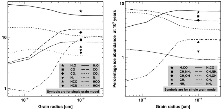
This mass transfer may result in a significant change in the ice composition depending on grain size. In Fig.5, we plot col-ored maps showing the percentage of ice abundance for selected species, with respect to the total ice abundance. For comparison, we show in Fig.6 the same maps but without the cosmic-ray-induced desorption. To complete the analysis, we show a simple line plot (see Fig.7) of the percentage ice abundances of the most abundant species as a function of grain radius at 106yr. In this figure, we also show the percentage ice abundance obtained with the single-grain-size model. The chemical composition on different grain sizes is indeed different when cosmic-ray-induced desorption is included, while it remains constant with grain size without it.

In general, the selected species can be divided into two groups by looking at their trends. In the first group we have CO, N2, HCO, H2CO and CH4, and in the second group we can put

all other species plotted here. The basic trend of species in the first group is that they have a lower percentage abundance on

(7)

A&A 615, A20 (2018)

Fig. 5.Percentage ice abundance of the most abundant species as a function of grain radius (x-axis) and time (y-axis). Results are for simulation with cosmic-ray-induced desorption enabled and for the MRN grain size distribution with 60 grain sizes. The dust temperature is kept constant at 10 K for all grains.

the small grains compared to the big grains. We also note that desorption energies of all these species are between 1100 K to 2100 K. In the second group we see a completely opposite trend, that is, the percentage abundance of all species is larger on the small grains and it decreases as the grain size increases. We also note that the desorption energy of all these species are above 5000 K except CO2whose desorption energy is 2575 K. Another

interesting point is that the percentage abundance as obtained in the single-grain model (see symbols in Fig.7) for the species of

the first group is lower than that in the multi-grain model for the same size grain (0.1 µm) while it is opposite for all species in the second group.

In Fig. 8, we show the gas-phase abundances of selected species for the above simulations. We see that the results with the single grain model, with or without the cosmic-ray-induced des-orption (in Fig.8, lines with stars and circles, respectively), are almost overlapping with the exception of N-bearing species and CH2OH; for these species curves very much overlap with each

(8)

Fig. 6.As in Fig.5but without cosmic-ray-induced desorption.

other until close to 5 × 105 _{yr where they begin to diverge. All}

of these species have a larger gas-phase abundance in the model with cosmic-ray-induced desorption. It is to be noted that gas phase CH2OH is mainly produced via CH3OH + CN → CH2OH

+ HCN reaction, and the increase in CH2OH production at later

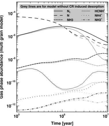
times is due to an increase in abundance of CN in the gas phase. Other N-bearing species, including CN, are increased in the gas phase because of higher gas phase abundances of N and N2. Our

analysis showed that, in the simulation with cosmic-ray-induced desorption, at about 5 × 105_{yr, almost 8% of N}

2production is

via the desorption of N2 ice, while this is almost nil when the

cosmic ray induced desorption is not included. This over satura-tion of N2 in the gas phase leads to an increase in abundances

of N and N+(N2+ He+→ He + N + N+). This finally results in

an increase in abundances of various N-bearing species such as CN, HCN, and many more (see Fig.9). Although we observed a noticeable impact of the cosmic-ray-induced desorption in the single-grain model for N-bearing species, for most other species the effect is not noticeable even up to 107yr.

In the multi-grain model, the gas phase abundance in most species is increased (see solid black lines in Fig. 8) due to the cosmic-ray-induced desorption and the differences in results for

(9)

A&A 615, A20 (2018)

Fig. 7.Percentage ice abundances of the most abundant species as a function of grain radius at 106 _{yr. Results are for the simulation with the}

cosmic-ray-induced desorption enabled and for the multi-grain model (lines), with 60 grain sizes and the MRN grain size distribution, and the single-grain model (symbols). The dust temperature is kept constant at 10 K for all grains.

the models with and without the cosmic-ray-induced desorption are even wider for N-bearing species (see Fig.10). In the multi-grain model, the effect of the cosmic-ray-induced desorption is noticeable even after 104_{yr while in the single-grain model it is}

visible only after 5 × 105yr. An increase in the abundance of one species can result in the decrease of another species, as can be seen with O2; its gas phase abundance is reduced in the

multi-grain model with the cosmic-ray-induced desorption while it is not noticeable in the single-grain model. In fact, the gas phase O2 is mainly reduced due to its increased destruction via two

reactions, CN + O2→ O + OCN and C + O2→ O + CO, as the

gas phase abundances of both CN and C are increased.

A greater abundance of species, such as CH3OH, which

mainly form on the grain surface, clearly indicates the effect of a more efficient desorption from the small grains at elevated tem-perature, although this elevated temperature stays for a very short time (only 10−5s) after each cosmic-ray collision before the sur-face temperature returns to normal. It should also be noted that the small grains are much higher in number (see Fig.2), meaning that any process which affects the small grains will show more prominent results overall.

To summarize, in this section, we explored the effect of the cosmic-ray-induced desorption in the single-grain and multi-grain models. We explained the differences in the ice compo-sitions on grains of different sizes due to the cosmic-ray-induced desorption. We showed that a more efficient desorption of physisorbed species from the small grains results in an increase in concentrations of certain species in the gas phase which in turn increases accretion rates causing big grains to gain more mass. Without the cosmic ray induced desorption, we did not see any change in the ice compositions on different grain sizes (in agreement withAcharyya et al. 2011;Pauly & Garrod 2016). We also observe that in the single grain model, the cosmic ray desorption process is a minor one for most of the species except N-bearing species so the results with or without it are very similar at least on the dust surface.

3.2. Grain number and effect of grain size distribution In this section, we explore the effect of varying the number of grain size bins in our model (1, 10, 30 or 60) and analyze how models with different grain size distribution (the MRN and the WD) compare to each other. We keep the surface temperature at 10 K for all grain sizes and the cosmic-ray-induced desorption is also enabled in all models.

Figure11shows the normalized total abundance of species on grain surface as a function of time. Here we have summed up the abundances of all species on all grain sizes in the multi-grain model to compare with the total ice abundance in the single-grain model. Further, to better visualize the effect of single-grain size distribution, we normalized the total ice abundance in all mod-els with the total ice abundance obtained in the single grain model. In both the MRN and the WD grain size distributions, we observe slight differences in the results due to a difference in the number of grains used in simulations. In both models, the total abundance using 30 bins and 60 bins is almost the same and slightly higher than when using 10 bins (black solid line for the MRN model and gray solid line for the WD model).

We see in Fig. 11 that initially (time <103 yr) the model MRN60, which has the highest total effective surface area (see Table1), has maximum ice. A higher surface area results in more accretion of gaseous species. At this early stage, the ice abun-dance is very low so the effect of cosmic-ray-induced desorption is not visible. But as ice abundance increases the effect of cosmic ray heating increases and we notice that relative abundance of ice in the MRN case becomes lower than that in the single-grain model and remains so until the end of the simulation. However, this relative change in abundance is not unidirectional. We see that the relative abundance in the MRN case starts increasing around 8 × 105 _{yr and then again at around 7 × 10}6 _{yr. But}

this trend is not sustained for long. This fluctuation in the rel-ative abundance may be because of a shortage of volatile species on the surface resulting in reduced desorption via the cosmic

(10)

Fig. 8.Gas phase abundances of selected species as a function of time. Solid and dashed black lines are for the multi-grain models with the cosmic-ray-induced desorption enabled and disabled, respectively. Gray lines with stars and circles, respectively, show the results from the single-grain model with and without the cosmic-ray-induced desorption. The dust temperature in each model is kept constant at 10 K for all grains. Legends apply to all panels.

ray hitting until the grains are populated again with the volatile species.

In the model with the WD grain size distribution, initial ice abundance is very low (about 25% only) compared to the other two models but it increases with time and comes very close to the total ice abundance in the single-grain model by the end of the simulation. The WD grain size distribution is very differ-ent from the MRN grain size distribution in two major ways. First, the total number density of grains is smaller by a large fac-tor resulting in a lower total effective surface area by a facfac-tor of almost 3.5. The effect of this is a lower ice production rate

under similar gas phase due to a lower accretion rate, so initial ice abundance is very low. Second, the total effective surface area of the small grains in the WD distribution is less than that of the big grains (see top panel in Fig.2) while in the MRN dis-tribution it is opposite. In other words, more ice is formed on the big grains than the small grains. The obvious effect of this is a reduced effect of the cosmic-ray collisions as ices on the small grains are affected the most by the cosmic ray collisions. We have seen that the gas phase abundance of N-bearing species is strongly affected by the cosmic-ray collisions with the dust grains.

(11)

A&A 615, A20 (2018)

Fig. 9.Simulated results of gas phase abundances of selected N-bearing species as a function of time as obtained in the single-grain model. Black and gray lines are for models with and without cosmic-ray-induced desorption, respectively. Dust temperature is kept constant at 10 K in both models.

In Fig. 12 we plot the gas phase abundances of a few N-bearing species for the WD case. We see that the differences in the results for models with and without the cosmic-ray-induced desorption are smaller than in the single grain model (Fig. 9). Specifically, the abundance of N2 and N is not affected as

strongly as seen earlier. After 3 × 106_{yr, the effect of the}

cosmic-ray-induced desorption starts to strongly affect the chemistry. This is expected as by this time there are lots of ices on the small grains which can desorb due to the cosmic-ray collisions.

Figure13shows the total ice abundances of selected species on the dust grains as a function of time for different grain size distributions and different bin numbers. In each multi-grain model, we summed the surface abundances of selected species over all grain sizes to get the total abundance of that species at any specific moment in time. The results of the model with the MRN distribution were discussed in great detail in the previous section. Here we note that the total ice abundances of H2O, CO2

and HCN in the MRN model are very similar to the single-grain model and higher than that in the WD model. In the previous section we saw that the ice compositions on different grain sizes are very different, with the small grains having a higher percent-age of heavier species and a lower percentpercent-age of lighter species, but, conversely, here we see that the total ice abundances of some species may remain similar in both the MRN model and the sin-gle grain model. The main difference between the models with the two different size distributions seems to be a shift in the time. In the model with the WD distribution, having a smaller total dust density and the surface area, the ices grow very slowly but at a very steady rate as depletion of gas phase species (and so the efficiency of the surface reactions) occurs at a much lower rate compared to the other two models. In the WD case, at the

Fig. 10.Gas phase abundances of selected N-bearing species as a func-tion of time as obtained in the multi-grain model with 60 bins and with the MRN grain size distribution. Black and grey lines are for the models with and without the cosmic-ray-induced desorption, respectively. The dust temperature is kept constant at 10 K in both models.

Fig. 11. Normalized total ice abundances as a function of time (see text). Cosmic-ray-induced desorption was enabled and the surface temperature was kept constant at 10 K in all models.

end of the simulation (107_{yr), the ice abundances of most of the}

species are more than that obtained in the MRN case. This is due to less efficient desorption via cosmic ray collisions in the WD

(12)

Fig. 12.As in Fig.10but for the simulation using the WD distribution. model. This helps in keeping most of the accreted matter on the grain surface.

When looking at the gas phase abundances (see Fig.14), we see that many species are more abundant in the WD case than in the simulation with the MRN distribution or the single grain size model. For the WD model, the species formed in the gas phase only, such as CO, CS, and O2, present a larger gas-phase

abun-dances as there are less grains to deplete them. On the contrary, species formed on the grains (such as CH3OH, HCOOCH3 or

CH3OCH3) have smaller abundances as there are less grains to

produce them. But abundances of these species start to increase significantly after 105_{yr and by the time the simulation reaches}

106 yr, most of these species have gas phase abundances much higher than that in the single grain model. This rapid gain in the gas phase abundances of certain species is due to the desorption from the small grains. For example, at 3 × 105yr, desorption of CH3OCH3ice from the smallest grain contributes almost 5% of

the production of CH3OCH3in the gas phase while the

contribu-tion of the second smallest grain is about 1.5%. This contribucontribu-tion is absent in the single-grain model. Simulations with the MRN distribution always give higher gas phase abundances for most of these species.

As a general result, the choice of grain size distribution can have a strong impact on the gas-phase abundances of some species. Simulation with the WD distribution shows that the small grains in the simulation can play a vital role at later times even if their number density is lower. Here, we also note that although using 10 grain sizes changes the results significantly over the single grain model irrespective of which type of grain size distribution is used, changing to 30 or 60 grain sizes has lit-tle impact. Although implementation of more processes which are grain-size-dependent, such as fluctuation in the surface tem-perature due to UV photons hitting the grains or nonuniform surface temperature, may result in very significant changes with more grain sizes.

3.3. Effect of dust-size-dependent surface temperature In the diffuse clouds, the surface temperature varies strongly with the grain size (Draine & Lee 1984) but in the dense cold clouds it is also well accepted that grains of different sizes have different temperatures. The surface temperature is an important parameter and can change the ice composition significantly. In this section, we explore the effect of considering a dust temper-ature that would depend on the size of the grains. The bottom panel in Fig.3shows the surface temperatures of the grains as a function of their radii used in the models. The grain temper-ature varies between 13.7 K (for the smallest 0.005 µm grains) and 11.1 K (for the biggest 0.25 µm grains). We note that in this model, the grain temperature of the single grain size model is 12 K (see Sect.2.2). A modification of the surface temperature effectively changes all the reaction rates on the surface but the diffusion of species with the smaller diffusion energies are the most affected because the diffusion rate increases exponentially with the surface temperature. Also, a change in the temperature affects mostly the chemistry in the top two layers as reactivity is small in the mantles.

Figure15shows the ice thickness at the end of simulations (107 yr) as a function of grain radius for different models: the single-grain model (symbols) and the multi-grain models with 10 (dashed lines) and 60 (solid lines) grain sizes (both the WD and the MRN distributions are shown). Here, we show two dif-ferent cases: 1) All grains are at the same temperature of 10 K (thin lines for the multi-grain model and star for the single-grain model), and 2) all grains have their own temperature (thick lines for the multi-grain model and a diamond for the single grain model). The ice thickness in the simulations with the WD dis-tribution is more than twice that in other models. This is because a smaller number density of grains results in more accretion on each grain size.

In the case of the size-dependent temperature model, the big grains have a temperature of about 11 K, which is a small dif-ference as compared to the model with grains at 10 K. This small difference has however a strong impact on the ice thick-ness for the WD model resulting in a difference of about 100 monolayers (i.e., 11% of the total ice thickness). This difference is even larger for the small grains. As the small grains have an even higher temperature than the big grains, the difference for the small grains between fixed and size-dependent temperature is larger. The effect is also seen for the MNR model in that case. We now compare the ice thickness for models with differ-ent numbers of bins (10 and 60). We see that in both (the MRN and the WD) multi-grain models with all grains at 10 K, the model with 10 bins has slightly higher ice thickness as com-pared to the model with 60 bins. But in the case of nonuniform surface temperature, big grains (radii >0.09 µm) in the model with 60 bins have more ices compared to big grains in the model with 10 grains. We assume that this is due to the difference in the bin sizes used in these models. We know that in the model with 60 bins, each bin is very small compared to the model with 10 bins, specially bins for big grains due to logarithmic division (see Fig.1). Keeping the bin size small helps in better approx-imation of the surface temperature as grains in a small bin can have temperatures that are very similar, but if the bin size is big, it may not be valid to assume that all grains in that bin are at the same temperature.

In the case of the WD model, the ice thickness is always smaller in the case of nonuniform temperature as compared to the 10 K model. For the MNR case, on the contrary, the mass transfer makes the curves cross for grains around 0.1 µm. For

(13)

A&A 615, A20 (2018)

Fig. 13.The total ice abundances of selected species on dust grains as a function of time for models with different grain size distributions and a different number of bins. Legends apply to all panels.

Fig. 14.Gas phase abundances of selected species as a function of time for models with different grain size distributions and a different number of bins. Legends apply to all panels.

the big grains, the ice thickness is larger with a nonuniform temperature as compared to the 10 K model.

Figure16shows colored maps of percentage ice abundances of selected species as a function of grain size and time in years for the model using the MRN distribution. We compared this figure with Fig.5in which the surface temperature is constant at 10 K for all grain sizes. We notice that the percentage of water on the small grains has reduced significantly. In this model, CO2

ice is the most abundant on the small grains, while in the model

with a uniform surface temperature H2O is the most abundant.

The percentage of CO2 ice has increased by more than a

fac-tor of two. We know that the obvious effect of higher surface temperature is an increase of hopping and desorption rates. In the case of CO2, this is essentially due to increased mobility of

O that results in more efficient production of CO2. Opposite to

this, a higher surface temperature increases the desorption rate of H2so significantly that water production goes down sharply. In

(14)

Fig. 15. The ice thickness as a function of grain radius at 107 _{yr in}

the different models. Thin lines: all grains have the same temperature of 10 K. Thick lines: all grains have their own temperature, see Fig.3. Cosmic ray induced desorption is used in all models.

change with grain radii and this change in the ice compositions are stronger than in the uniform surface temperature case. To see the effect of this on the total ice productions of various species, we plot, in Fig.17, the total abundances of selected species on the dust grains as a function of time for different models with grain-size-dependent temperature. Here we can clearly see that, in the MRN case, the total ice abundance of water has gone down com-pared to the model with uniform surface temperature while the same for CO2has gone up (see Fig.13for comparison). The total

abundance of water ice is almost unchanged in the single-grain model and the WD distribution, while the CO2 ice abundance

has increased but not very significantly. This is because the small grains play a major role in determining ice composition in the MRN model. The total ice abundance of most of the species has decreased due to the higher surface temperature. We also notice that, for a few species, results with 10 and 60 grain sizes do not overlap, which was the case in the previous results for the uni-form surface temperature. Differences are especially visible for CH4and CH3OH.

Figure 18 shows the gas phase abundances for selected species as a function of time for different models with grain-size-dependent temperature. We see very similar effects in the gas phase. The abundance of CO has increased in the MRN case as compared to Fig.14(uniform 10 K grain temperature) while it is almost unchanged for the WD models. Abundance of CH3OH

has decreased as it is now produced less efficiently on grains due to the higher desorption rate of adsorbed H atoms. Species that are mainly formed in gas phase, such as H2CO or HCOOCH3,

have higher abundances.

4. Comparison with observations in cold dense clouds

We compared our results obtained from different models with observations in the cold dense clouds TMC-1 and L134N. For

comparison, we used the method described in Loison et al.

(2014). We have computed the mean distance of disagreement D(t) for each output at time t of the simulation using the following formula

D(t) = 1 Nobs

X

i

|[log[n(Xi, t)] − log[n(Xiobs)]]|, (3)

where n(Xi, t) is the calculated abundance of species Xiat time t ,

n(Xobs

i ) is the observed abundance for the same species, and Nobs

is the total number of observed species used in the calculation of D(t). In this method, the smaller the value of D(t), the better the agreement between the observed abundances and the simulated results. We used tabulated data inAgúndez & Wakelam(2013) for observation data. From the table we used abundances of 34 molecules for L134N and 52 molecules for TMC-1; we did not consider species for which only upper or lower limits are given.

Figure 19shows the calculated mean distance of disagree-ment from the observed abundances in the two clouds as a function of time as obtained from the single-grain and multi-grain models. First we will discuss the case of TMC-1. We see that all models give the best agreement with the observation at about 2 × 105 _{yr. At this time, the multi-grain model with the}

MRN distribution (black dashed and dotted lines) gives the best agreement followed by the single grain model (black solid line). After reaching this point of best agreement, both the single-grain model and the multi-single-grain model with the WD distribution deviate away and cross the line where the mean distance of dis-agreement becomes more than two, while the multi-grain model with the MRN distribution remains best. The multi-grain model with the WD distribution again returns to the best agreement at about 2 × 106_{yr. In the multi-grain models, we see that the model}

with nonuniform surface temperatures (dotted lines) gives the best agreement for both the MRN and the WD distributions. The reason why the multi-grain models stay close to the best value while the single-grain model does not is again due to basic differ-ences in the two models. The single-grain model lacks a proper desorption mechanism for the ices. Due to this there is no way to cycle material from the gas to the grain and then back to the gas. This results in a gradual increase in the ice abundance only. So after reaching a state of the best agreement there is no way that it can fluctuate around it. In the multi-grain model, due to the presence of a large number of small grains, we have a bet-ter desorption mechanism in the form of the cosmic-ray-induced desorption that results in a cycle of material from the grains to the gas.

We see a very similar result in the case of L134N. All models give a very good value of D(t) at around 6 × 105_{yr. At this time}

D(t) is less than one for all models. This means that the mean difference between modeled and observed abundances is smaller than a factor of ten. This case also shows that the multi-grain model with the WD distribution gives better agreement than the same model with the MRN distribution. This essentially shows how different types of grain size distribution can lead to differing estimates of the observed abundance in different clouds.

5. Discussion on the cooling of grains after a collision with cosmic ray particles

The cooling of the grains after the collisions with cosmic-ray particles is assumed to be the most efficient by the evapora-tion of the surface species. The cooling time of 10−5 s esti-mated by Hasegawa & Herbst (1993a; see also Sect. 2.2 and

(15)

A&A 615, A20 (2018)

Fig. 16.Percentage ice abundances of the most abundant species as a function of grain size (x-axis) and time (y-axis). Results are for the multi grain model with 60 grain sizes and with non-uniform surface temperatures. The cosmic-ray-induced desorption is used and the MRN grain size distribution was used to calculate number density of 60 grain bins.

Herbst & Cuppen 2006) is based on the assumption that the

grains are covered by a significant number of CO molecules. We have shown that the small grains are depleted in light species such as CO due to the higher temperatures with respect to the larger grains. Since other abundant ice species (H2O, N2, CH4,

CO2, or CH3OH) have higher desorption energies, the cooling

of the smallest grains may take longer than what is assumed here.

To test the sensitivity of the model to this, we have scaled the duration of the temperature peaks produced by the cosmic ray collisions for grains smaller than 0.1 µm. In fact the small

grains have less sites so less possibility for CO to desorb. For the scaling, we used a simple factor given by 106_/N

s(i), where Ns(i)

is the number of sites on the ith grain. Using this scaling, the desorption from the small grains is more efficient. Looking at the complex organic molecules observed in the cold cores, this additional nonthermal desorption may increase their gas phase abundances. All of these complex organic molecules (COMs) are, however, not necessarily produced enough on the grains, or, rather, are more abundant on the big grains than on the small ones. Here we do not take into account the composition of the grains themselves (i.e., the presence of CO).

(16)

Fig. 17.Total ice abundances of selected species on dust grains as a function of time for the models with different grain size distributions and different number of bins. Grain temperature is non-uniform in the multi grain models and in the single grain model surface temperature is 12 K. Legends apply to all panels.

Fig. 18.Gas phase abundances of selected species as a function of time for models with different grain size distributions and a different number of bins. Grain temperature is nonuniform in the multi-grain models and in the single-grain model surface temperature is 12 K. This legend applies to all panels.

In our model, methanol is very abundant on small grains and more desorption from the small grains could account for the observed gas phase abundances (Öberg et al. 2010). Similar results were found for CH3O, CH3CCH, HCOOH,

and CH3OCH3. But while CH3CHO is mostly present on big

grains (>0.02 µm), the ice abundances of HCOOCH3 on grains

(whatever the size) are too low to account for the observed gas phase abundances.

6. Conclusions

Here we summarize our main findings from this work.

We observe very small differences in the results when switching from 10 grain sizes to 30 grain sizes in our models and almost no difference in the results for simulations with 30 grain sizes and 60 grain sizes. Therefore, for both the MRN and the WD models, one can use up to 30 grain sizes if better preci-sion is needed and there is almost no need to go above 30 grain

(17)

A&A 615, A20 (2018)

Fig. 19.Mean distance of disagreement computed for two dark clouds TMC-1 network and L134N.

sizes. This result may change if one tries with some other grain size distribution model or stochastic heating of dust grains.

Results from the single-grain and multi-grain models both using the MRN distribution are very close and are similar in absence of the cosmic rays provided all grains are at the same surface temperature. This is due to a very similar total effective surface area in both the models.

The collisions of the cosmic ray particles with the small grains (<0.04 µm) causes the evaporation of a large portion of the ices from the surfaces. This results in a significant reduc-tion in the ice thickness on these grains. The evaporated species then accrete again on the surfaces of the big grains, on which the cosmic ray induced peak temperature is much smaller. The cosmic-ray-induced desorption thus produces a mass transfer of ices from smaller to bigger grains. The mass transfer is even more efficient when the size dependency of the dust temperature is considered.

The choice of the MRN or the WD distributions strongly affects the abundances of most of the species. The cosmic-ray-induced desorption is the most effective in the MRN distribution case. In the WD distribution case, a larger contribution to the total effective surface area comes from big grains, and therefore most of the ices are formed on the big grains. Also, for most species, the cosmic-ray-induced desorption of the ices brings about noticeable changes in the gas phase abundances after 106 _{yr only when there are significant ice abundances on the}

small grains. Most of the species have smaller ice abundances in the WD case due to a lower number density of dust grains as compared to the MRN distribution.

Ice composition is dependent on grain size. Ices on the small grains contain a small percentage of lighter molecules, such as CO, HCO and N2, and a larger percentages of more strongly

bound species, such as water and CO2.

Considering a nonuniform surface temperature for the differ-ent grain sizes strongly impacts the overall gas and ice composi-tions. The difference in the chemical compositions between the small and big grains is even stronger.

The MRN distribution gives a better agreement with TMC-1 observations whether the dust temperature is uniform or not, while both the MNR and the WD distributions give a better agreement with L134N when dust temperature is nonuniform.

Acknowledgements.This study has received financial support from the French State in the frame of the “Investments for the future” Programme IdEx Bordeaux, reference ANR-10-IDEX-03-02. VW research is funded by an ERC Starting Grant (3DICE, grant agreement 336474) and the CNRS program Physique et Chimie du Milieu Interstellaire (PCMI) co-funded by the Centre National d’Etudes Spatiales (CNES). V.W. thanks Bruce Draine for helpful discussions. References

Acharyya, K., Hassel, G. E., & Herbst, E. 2011,ApJ, 732, 73

Agúndez, M., & Wakelam, V. 2013,Chem. Rev., 113, 8710

Draine, B. T., & Lee, H. M. 1984,ApJ, 285, 89

Garrod, R. T. 2008,A&A, 491, 239

Ge, J. X., He, J. H., & Li, A. 2016,MNRAS, 460, L50

Graedel, T. E., Langer, W. D., & Frerking, M. A. 1982,ApJS, 48, 321

Hasegawa, T. I., & Herbst, E. 1993a,MNRAS, 261, 83

Hasegawa, T. I., & Herbst, E. 1993b,MNRAS, 263, 589

Hasegawa, T. I., Herbst, E., & Leung, C. M. 1992,ApJS, 82, 167

Herbst, E., & Cuppen, H. M. 2006,Proc. Natl. Acad. Sci., 103, 12257

Hincelin, U., Wakelam, V., Hersant, F., et al. 2011,A&A, 530, A61

Iqbal, W., Acharyya, K., & Herbst, E. 2014,ApJ, 784, 139