HAL Id: hal-00297643
https://hal.archives-ouvertes.fr/hal-00297643
Submitted on 31 Aug 2007
HAL is a multi-disciplinary open access
archive for the deposit and dissemination of
sci-entific research documents, whether they are
pub-lished or not. The documents may come from
teaching and research institutions in France or
abroad, or from public or private research centers.
L’archive ouverte pluridisciplinaire HAL, est
destinée au dépôt et à la diffusion de documents
scientifiques de niveau recherche, publiés ou non,
émanant des établissements d’enseignement et de
recherche français ou étrangers, des laboratoires
publics ou privés.
Suitability of quantum cascade laser spectroscopy for
CH4 and N2O eddy covariance flux measurements
P. S. Kroon, A. Hensen, H. J. J. Jonker, M. S. Zahniser, W. H. van ’T Veen,
A. T. Vermeulen
To cite this version:
P. S. Kroon, A. Hensen, H. J. J. Jonker, M. S. Zahniser, W. H. van ’T Veen, et al.. Suitability of
quan-tum cascade laser spectroscopy for CH4 and N2O eddy covariance flux measurements. Biogeosciences,
European Geosciences Union, 2007, 4 (5), pp.715-728. �hal-00297643�
www.biogeosciences.net/4/715/2007/ © Author(s) 2007. This work is licensed under a Creative Commons License.
Biogeosciences
Suitability of quantum cascade laser spectroscopy for CH
4
and N
2
O
eddy covariance flux measurements
P. S. Kroon1, A. Hensen1, H. J. J. Jonker2, M. S. Zahniser3, W. H. van ’t Veen1, and A. T. Vermeulen1
1Energy Research Centre of the Netherlands (ECN), Department of Air Quality and Climate Change, The Netherlands 2TU Delft, Department of Multi-Scale Physics, Research Group Clouds, Climate and Air Quality, The Netherlands 3Aerodyne Research, Inc., USA
Received: 20 March 2007 – Published in Biogeosciences Discuss.: 12 April 2007 Revised: 22 August 2007 – Accepted: 29 August 2007 – Published: 31 August 2007
Abstract. A quantum cascade laser spectrometer was eval-uated for eddy covariance flux measurements of CH4 and
N2O using three months of continuous measurements at a
field site. The required criteria for eddy covariance flux mea-surements including continuity, sampling frequency, preci-sion and stationarity were examined. The system operated continuously at a dairy farm on peat grassland in the Nether-lands from 17 August to 6 November 2006. An automatic liquid nitrogen filling system for the infrared detector was employed to provide unattended operation of the system. The electronic sampling frequency was 10 Hz, however, the flow response time was 0.08 s, which corresponds to a bandwidth of 2 Hz. A precision of 2.9 and 0.5 ppb Hz−1/2was obtained for CH4 and N2O, respectively. Accuracy was assured by
frequent calibrations using low and high standard additions. Drifts in the system were compensated by using a 120 s run-ning mean filter. The average CH4and N2O exchange was
512 ngC m−2s−1 (2.46 mg m−2hr−1) and 52 ngN m−2s−1 (0.29 mg m−2hr−1). Given that 40% of the total N2O
emis-sion was due to a fertilizing event.
1 Introduction
The greenhouse gasses methane (CH4) and nitrous oxide
(N2O) play an important role in global warming with global
warming potentials 23 and 296 times greater than CO2 for
100 years time horizon (IPCC, 2001). Agricultural soils are major sources of both gasses (IPCC, 2006). Although, there are significant uncertainties in the estimated CH4 and
N2O fluxes, mainly owing to a combination of complexity of
the source (i.e. spatial and temporal variation), limitations in the measurement equipment and the methodology used to quantify emissions. High-frequency micrometeorological
Correspondence to: P. S. Kroon
methods are often used to determine integrated emission es-timates on a hectare scale that also have continuous cover-age in time. Instrumentation is now becoming available that meets the requirements for CH4and N2O eddy covariance
(EC) measurements. For example, a limited number of EC measurements have been published using lead salt tunable diode laser (TDL) spectrometers and quantum cascade lasers (QCL) spectrometers (e.g. Smith et al., 1994; Wienhold et al., 1994; Laville et al., 1999; Hargreaves et al., 2001; Werle and Kormann, 2001; Eugster et al., 2007; Neftel et al., 2007).
A TDL spectrometer can obtain similar precision as a QCL spectrometer, however, the big advantage of QCL spectrome-ters are the better laser frequency stability and freedom from cryogenic cooling cycles that can lead to instability in mode purity and laser frequency. The QCL was first demonstrated in 1994 (Faist et al., 1994). Several studies are performed using QCL spectroscopy e.g. by Nelson et al. (2002) and Jim´enez et al. (2005). Nelson et al. (2004) pointed out that the system must satisfy four criteria for performing CH4and
N2O EC measurements. First, the continuity criteria which
means that the system should be able to operate unattended on a continous basis at a remote field site. Second, the an-alyzer response time and the electronic sampling frequency should be both on the order of 10 Hz to evaluate the small eddies as well (Monteith and Unsworth, 1990). Third, the precision of the concentration measurements should be a few parts per thousand of the ambient mixing ratio for CH4and
one part per thousand for N2O. A required precision of 4 ppb
and 0.3 ppb is derived for CH4and N2O given an average
am-bient concentration of 1800 ppb and 320 ppb. Finally, the sta-tionarity criteria that indicates the requirement of intermedi-ate term stability against span and minimal drift during a pe-riod of atmospheric stationarity on the order of 30 min. Nel-son et al. (2004) showed that QCL spectrometers can meet these criteria. This conclusion is mainly based on an exper-iment with which the system was located in the laboratory. Therefore, it is desirable to validate the suitability of a QCL
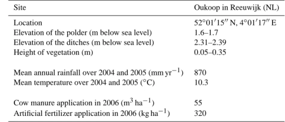
Table 1. Main characteristics of Oukoop site in Reeuwijk based on e.g. Veenendaal et al. (2007).
Site Oukoop in Reeuwijk (NL)
Location 52◦01′15′′N, 4◦01′17′′E Elevation of the polder (m below sea level) 1.6–1.7
Elevation of the ditches (m below sea level) 2.31–2.39 Height of vegetation (m) 0.05–0.35 Mean annual rainfall over 2004 and 2005 (mm yr−1) 870 Mean temperature over 2004 and 2005 (◦C) 10.3 Cow manure application in 2006 (m3ha−1) 55 Artificial fertilizer application in 2006 (kg ha−1) 320
spectrometer for EC measurements at a remote field site. This paper discusses the performance of QCL spectrom-eters for EC measurements using three months of continu-ous measurements at a dairy farm on peat grasslands in the Netherlands. Moreover, an estimate will be given of CH4
and N2O exchange. A description of the experimental site
and the climatic conditions is given in Sect. 2. Section 3 is devoted to the instrumentation and the methodology. The re-sults are shown in Sect. 4. The conclusions and discussions are presented in Sect. 5.
2 Experimental site and climatic conditions
The measurements were performed at an intensively man-aged dairy farm. This farm is located at Oukoop near the town of Reeuwijk in the Netherlands (Coord 52◦01′15′′N, 4◦01′17′′E). The surrounding area of the measurement loca-tion has soil consisting of a clayey peat or peaty clay layer of up to 0.25 m on up to 12 m eutrophic peat deposits. Rye grass (Lolium perenne) is the most dominate grass species with rough bluegrass (Poa trivialis) often co-dominant. Clover species constitute less than 1% of the vegetation (Veenen-daal et al., 2007). About 21% of the area is open water (Nol et al., 20071). The site is located in a polder which means that the water level can be managed. The mean elevation of the polder is between 1.6 and 1.8 m below sea level. Ditch water level in the polder is being kept at−2.39 in winter and −2.31 m in summer (Veenendaal et al., 2007). The climate is
temperate and wet, with an average temperature of 10.3◦C in 2004 and 2005, and with an averagely annual precipitation of about 870 mm in 2004 and 2005. The dominating wind direction is southwest (Veenendaal et al., 2007). A summary of the main characteristics is given in Table 1.
Manure and fertilizer are applied about five times a year from February to September. Besides, there are also about
1Nol, L. et al.: Effect of land cover data on N
2O inventory in fen
meadows, J. Environ. Qual., submitted, 2007.
five harvest events. Manure and artificial fertilizer appli-cation were about 55 m3ha−1yr−1(253 kgN ha−1yr−1) and 320 kg ha−1yr−1 (84 kgN ha−1yr−1) in 2006. The system operated continuously (coverage of 87%) from 17 August to 6 November 2006. The average temperature over the mea-surement period was 17◦C and 55 kgN ha−1cow manure was applied on 14 September 2006.
3 Instrumentation and methodology 3.1 Instrumentation
The QCL spectrometer was placed in a container of 2×2×2 m at about 20 m east from the mast. The measure-ment height was 3 m and the mast was positioned in the mid-dle of the field. Terrain around the towers was flat and free of obstruction for at least 600 m in all directions, except for the container. Wind speed, air temperature, CH4 and N2O
concentrations were measured with a system consisting of a three-dimensional sonic anemometer (model R3, Gill In-struments, Lymington, UK) and a QCL spectrometer (model QCL-TILDAS-76, Aerodyne Research Inc., Billerica MA, USA).
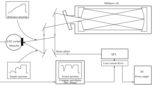
Figure 1 shows a schematic view of the QCL spectrom-eter. The QCL spectrometer has a multipass cell with an optical path of 76 m and a volume of 0.5 l maintained be-tween 4.7×10³Pa (35 Torr) and 4.3×10³Pa (40 Torr). The
QCL spectrometer has two laser positions available that can be used simultaneously. During these experiments only one laser was used which operated at the 1270.8 and 1271.1 cm−1 absorption lines for CH4and N2O, respectively. The
perfor-mance of the system will be influenced by the use of the sec-ond laser. The use of two lasers affects the electronic sam-pling frequency. Besides, the penalty in signal-noise ratio would be proportionally smaller by the square root of the duty cycle difference (the amount of measurements). If two lasers are sharing the same sweep equally, the signal-noise ratio on both will be increased by√2. The reason for not
LN2 cooled Detector
Laser current driver
DC Power supply Beam splitter
Reference spectrum
TDL−Wintel Computer and display
Sample spectrum Scaled spectrum
Multipass cell
QCL
Fig. 1. Schematic view of the QCL spectrometer based on Nelson et al. (2004).
using the second laser in this case was to maximize the sig-nal to noise ratio, which requires the most precision for flux measurements.
The laser was used in pulsed mode. A sequence of laser light pulses, each with duration of about 10 ns, is divided by a beam splitter and sent through the multipass cell and along a bypass. Both beams are detected on a single detec-tor sequentially with the bypass pulse arriving 250 ns before the multipass pulse. The laser frequency is tuned through the absorption lines using a sub-threshold current applied to laser between pulses. The laser light intensity is lower at the start of the pulse sequence and increases towards the end of the pulse sequence. The total width of the scan is close to 0.5 cm−1This is true for both beams. The bypass signal is used to normalise the signal obtained from the multipass cell. The result is a pattern that shows a relatively constant inten-sity ratio with a decrease in light inteninten-sity passing through the multipass cell at the frequencies of the two absorption lines.
The QCL software, TDL-Wintel, uses spectral parameters listed in the HITRAN database to make a fit to this pattern and derive approximate CH4 and N2O gas concentrations
(Rothman and Barbe, 2003). With pulsed QCLs, the laser line width is on the same order as the Voigt line width of the absorber, and therefore must be considered in the fitting routine by convolving the laser line shape with the molec-ular absorbance. The non-Gaussian shape of the laser line profile can result in underestimating the molecular concen-tration from 10 to 20% depending on the line depth. Calibra-tion with known standards is therefore necessary for greater accuracy.
The detectors of the QCL spectrometer require cooling by liquid nitrogen for maximum sensitivity in the wavelength region. The 0.5 l dewar on the optical table needs to be
re-filled approximately every 24 h. An automated filling unit was used (with a 50 l storage dewar produced by Norhoff, Netherlands). With this setup visits to the instrument were necessary only once a week. In order to minimize drift ow-ing to changow-ing alignment the temperature cover and optical table were maintained at 35±0.1◦C by thin film heaters. The laser electronics were stabilized at±0.1◦C using circulating water bath (Nelson et al., 2004). The water cooling circuit is primarily used to remove the heat generated by the peltier element, which cools the laser. It also stabilizes the tempera-ture of the pulse electronics to provide a more uniform laser output power, and it stabilizes the position of the laser which rest on the peltier element. Without water cooling a variation in reported mixing ratios can occur when ambient tempera-ture surpasses the system temperatempera-ture as large as 2 ppb◦C−1 for N2O (Nelson et al., 2004).
The air inlet was located at the sonic height of 3 m above the field. A 25 m PTFE inlet tube with a diameter of 0.25 inch was used. At the QCL spectrometer inlet a 0.01 µm filter (DFU filter tube grade BQ, Balston, USA) was used to avoid degradation of the multipass cell mirrors. The flow and cell pressure were controlled with a needle valve at the inlet of the multipass cell. A vacuum pump (TriScoll 600, Varian Inc, USA) with a maximum volume flow rate of 400 l min−1was located downstream of the multipass cell. The QCL spec-trometer was calibrated at least once a week using mixtures in N2/O2of 1700 and 5100 ppb for CH4and 300 and 610 ppb
for N2O (Scott speciality gasses, Netherlands)
The sonic anemometer data and the QCL spectrometer output were logged using the RS232 output and processed using a data acquisition program developed at ECN, fol-lowing the procedures of McMillen (1988). Both the QCL spectrometer computer and the EC computer were available for remote control. The electronic sampling frequency of
the QCL spectrometer was not exactly uniform. The aver-age time between two samples was about 0.11 s. The sonic anemometer produced an uniform sampling rate of 20.88 Hz. The data acquisition program saved both the QCL spectrom-eter and sonic anemomspectrom-eter data in the same file at 20.88 Hz using the last measured concentration value.
3.2 Methods
The net ecosystem exchange (NEE) consists of the sources, the sinks and the surface flux. Horizontal homogeneity, a flat terrain and stationary circumstances were assumed within the average time of 30 min. The storage term was calculated us-ing the average values of CH4 and N2O at 3 m height over
each 30 min period. The net ecosystem exchange over 30 min of both gasses is given by
Z h 0 Scdz | {z } NEE = ci− ci−1 T h | {z } Storage + w′c′|h | {z } Eddy flux (1)
in which h is the measurement height in m, Scis the source term in ppb s−1, c is the gas concentration of CH4 or N2O
in ppb, i indicates the flux number, T is the average time in s and w is the vertical wind velocity in m s−1(e.g. based on Hoogendoorn and van der Meer, 1991 and Nieuwstadt, 1998).
Evaluation of the eddy flux consisted of different phases. First, the raw data of w(t ) and c(t ) was analyzed by eye on spikes and malfunctioning. This evaluation was chosen to look in more detail into the data, however, it is very imprac-tical for long term flux measurements. The raw data screen-ing should be done automatically in further research. Then, all concentration data was corrected using a two-point cali-bration factor based on weekly calicali-brations. The two-point calibration factor fLHis defined by
fLH=
SH− SL
MH− ML
(2)
in which SLand SHare the low and high standard values in
ppb and MLand MHare the low and high measured values in
ppb. The corrected concentration was found using this factor and the following equation
Ccor= fLHCuncor (3)
with Cuncorthe uncorrected concentration value in ppb and
Ccor the corrected concentration value in ppb. It was
im-portant to correct the data using this factor since the QCL spectrometer does not provide absolute values for the mixing ratios. Next, the time average, which was based on a running mean, and mean removal operations were performed by
˜ wk= (1 − 1t τf )w˜k−1+ 1t τf wk (4) ˜ck= (1 − 1t τf )˜ck−1+ 1t τf ck (5) w′c′= 1 ns ns X k=1 (wk− ˜wk)(ck− ˜ck). (6)
where k is the sampling number, 1t is the interval between two samples in s, τf is the running mean filter time constant in s and ns is the amount of samples in the average period
(Lee et al., 2004). The eddy fluxes Fc were calculated us-ing a 120 s runnus-ing mean filter time constant and a 30 min average time. Furthermore, the time lag between the sonic anemometer and QCL spectrometer data caused by the length of the sampling tube was determined using the covariance as function of delay time, which is given by
Fc = covwc(n1t)= w′kc′k+n1t= 1 ns ns X k=1 w′kc′k+n1t (7)
where the delay time is defined by n1t in which n denotes the amount of time steps. The absolute maximum in covari-ance, which represents the eddy flux, occurs at the exact de-lay time. The exact dede-lay time is dependent on the flow rate in the tube. The flow rate itself is dependent on the resistance of the system, which is mainly dependent on the conditions of the inlet filter. If the inlet filter becomes dirty, the flow rate will decrease.
The storage term was calculated using the QCL spectrom-eter data according to Eq. (1). The calibrated corrected NEE was given by adding the storage and the eddy flux term. Furthermore, the Webb-correction was partly applied (Webb et al., 1980). The Webb-correction for density fluctuations was not performed since there was a constant temperature and pressure in the sampling cell. However, the Webb-correction for the influence of water vapour fluctuations on trace gas fluxes was applied on the data since the sample was not dried to a constant humidity before the mixing ratio was measured. The Webb-correction was performed using latent heat flux data of the University of Wageningen. These latent heat fluxes were derived using an open path system which was located at the same height and at a distance of about 3 m from the closed path EC system of CH4and N2O. The
Webb-correction based on this open path EC system probably over-estimated the correction because the 25 m inlet tube of the closed EC system of CH4 and N2O attenuated the fluxes.
For more information about the open path system the reader is referred to Veenendaal et al. (2007). Moreover, the NEE data were flagged using the instationarity test of Foken and Wichura (1996). Finally, the fetch was checked by a foot-print model based on the Kormann-Meixner method (Neftel et al., 20072; Kormann and Meixner, 2001). The 30 min NEE value was rejected when less than 70% of the flux came from the dairy farm site.
2Neftel, A. et al.: A simple tool for operational footprint
4 Results
4.1 Performance EC measurements
The required criteria for EC flux measurements including continuity, sampling frequency, precision and stationarity were examined using three months of field measurements. First, the continuity of the system was evaluated. The system operated continuously (total data coverage 87%) at a dairy farm on peat grassland in the Netherlands from 17 August to 6 November 2006 with about one visit per week excluding the intensive campaigns. The system proved to be very sta-ble as far as alignment and laser drift was concerned. The most sensitive part of the system proved to be the liquid nitrogen refilling unit. In summer with high temperatures the container became too hot inside which led to changing alignment. An extra ventilator was installed on the container which proved to be sufficient to keep the temperature inside the container below 35◦C.
The validation of the sampling frequency of the system consisted of three parts, namely the electronic sampling fre-quency, the flow response and the damping. For most con-ditions a sampling frequency of about 10 Hz is sufficient to perform EC measurements (Ammann, 1998). The electronic sampling frequency is dependent on the complexity of the spectrum and the number of spectral lines included in the fit. Laboratory tests, using the Aerodyne TDL-Wintel soft-ware running on a 1 GHz PC showed that 20 Hz acquisition was possible for 2 or 3 gas species simultaneously. Two species were simultaneously measured at an adjusted elec-tronic sampling frequency of 10 Hz during the continuously field measurements. The average time between two samples was about 0.11 s. As a consequence, the contribution to CH4
and N2O fluxes of large eddies, with sampling frequencies
below 5 Hz, were electronically sampled well, but the contri-bution of smaller eddies were not.
However, the overall sampling frequency of the system is limited by sampling cell response time rather than the sig-nal processing time. A sampling cell response time (1/e) of τ =0.08 s was obtained using the 400 l min−1Varian vac-uum pump with a cell volume of 0.5 l in the laboratory. The measured response time implies a volume flow rate of 375 l min−1which is close to the nominal pumping speed. The response time was not determined in the field since no automatic calibration system was installed. However, the re-sponse time in the laboratory and in the field should be prob-ably the same since it should not be a function of the flow rate as long as the pumping speed is constant with the cell pressure. Thus, the effective bandwidth 1/(2π τ ) is estimated at∼2 Hz which is slightly less than the Nyquist frequency of 5 Hz using a sampling rate of 10 Hz.
Nevertheless, the contribution of high frequencies (i.e. the small eddies) to the calculated flux can be decreased by the inlet tube. According to Lenschow and Mann (1994) the damping effect was estimated to be smaller than 50%
for frequencies below 3 Hz when cell pressures were above 4.7×10³Pa (35 Torr). In that case, the Reynolds number was higher than 4000. The flow was prevented from becoming less turbulent by regular replacement of the inlet filters. A thorough investigation on the damping effect could be done using an empirical correction approach given by Ammann et al. (2006). This correction approach is based on a com-parison of the normalized co-spectrum of wT and wCH4or
wN2O. The wT co-spectrum is calculated from the sonic
anemometer with which almost no damping occurred. An es-timation of the damping is done using the flux ogives which are given by OgwcD (fm)= m X i=1 |Cowc(fi)| fi= i (ns− 1)1t; m = 1, 2, ..., h (ns− 1)1t 21t i (8)
where f represents frequency in Hz and Cowc the normal-ized co-spectrum. The ogive represents the true cumulative contribution of the turbulent eddy frequencies to the flux. The total damping effect is determined by scaling the damped ogive at the low frequencies (up to 0.065 Hz which means a time period of 15 s) to the respective undamped ogive of
wT . The damping factor is then indicated by the right-end of
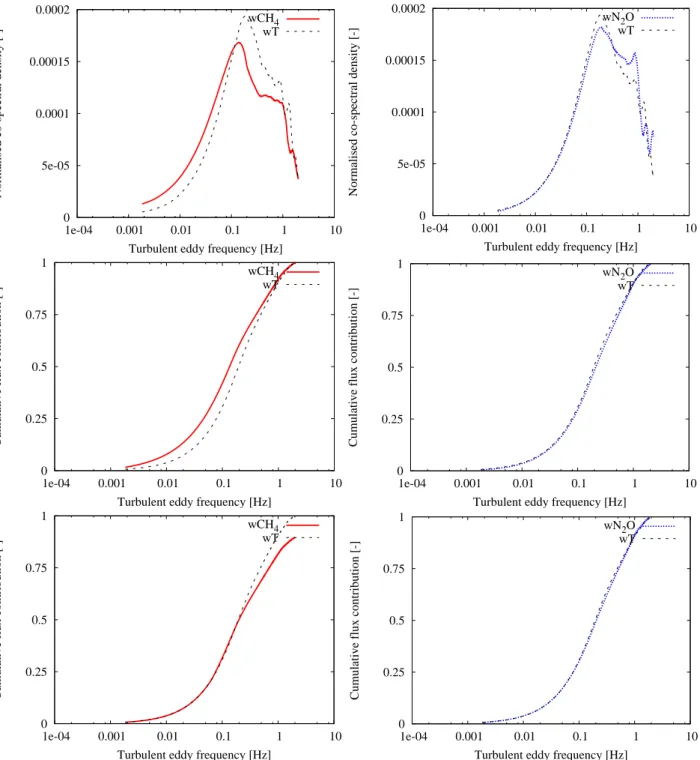
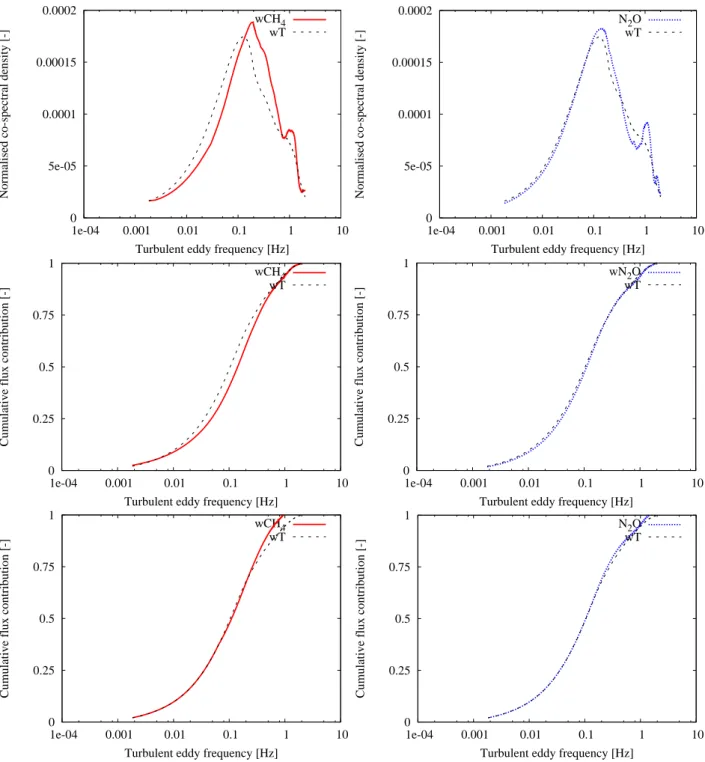
the ogive. Figure 2 and 3 show the absolute normalized co-spectra of CH4, N2O and wT belonging to 7 October 2006
between 12:00–14:00 which was a neutral period with mean wind velocity of about 7 m s−1and 8 October 2006 between 00:00–02:00 which was a stable period with mean wind ve-locity of about 3 m s−1. Besides, the unscaled and scaled ogives are presented in these figures. These analyses were determined using block averaging instead of a running mean filter and an average time of 30 min. The contributions until a sampling frequency of 2 Hz were taken into account. It can be seen that there is almost no difference between the contri-bution at the high frequencies of the wT flux and the wCH4
or wN2O flux. Therefore, the damping effects seem to be
almost negligible. Although, more analyses should be done to investigate the effect of damping on the flux values for all circumstances.
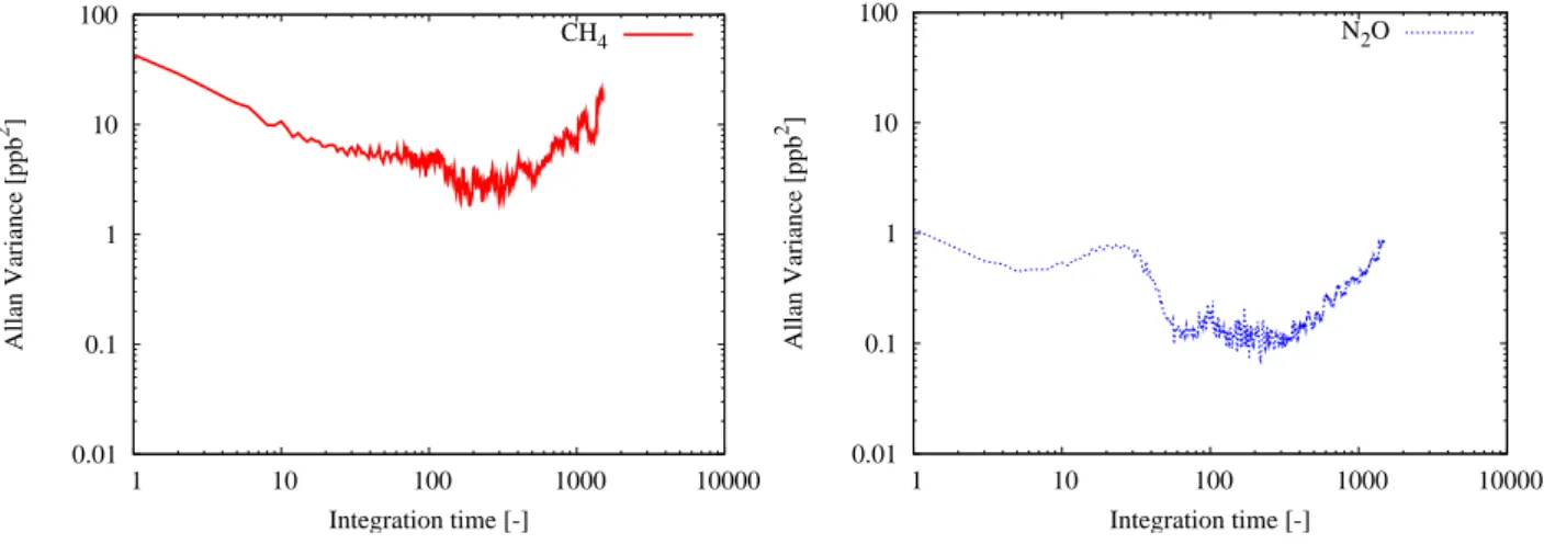
The system precision and stationarity are strongly depen-dent on the drift of the instrument. An indication of both properties can be given using an Allan variance analysis (e.g. Allan, 1966; Werle and Slemr, 1991). In this method, the variances in the time series of reported mixing ratio when sampling a constant source from a calibration take are plot-ted as a function of integration time. The Allan variance de-creases with t−1 when random noise dominates. This de-crease continues to a point at which drift effects start to in-fluence the measurements. Due to instrument drift at longer times the Allan variance increases again. The minimum is indicated by τA and σA, which represent the stability time
in s and the sensitivity in ppb Hz−1/2belonging to this sta-bility time. Apart from this, the y-axis intersection point
0 5e-05 0.0001 0.00015 0.0002 1e-04 0.001 0.01 0.1 1 10
Normalised co-spectral density [-]
Turbulent eddy frequency [Hz] wCH4 wT 0 5e-05 0.0001 0.00015 0.0002 1e-04 0.001 0.01 0.1 1 10
Normalised co-spectral density [-]
Turbulent eddy frequency [Hz] wN2O wT 0 0.25 0.5 0.75 1 1e-04 0.001 0.01 0.1 1 10
Cumulative flux contribution [-]
Turbulent eddy frequency [Hz] wCH4 wT 0 0.25 0.5 0.75 1 1e-04 0.001 0.01 0.1 1 10
Cumulative flux contribution [-]
Turbulent eddy frequency [Hz] wN2O wT 0 0.25 0.5 0.75 1 1e-04 0.001 0.01 0.1 1 10
Cumulative flux contribution [-]
Turbulent eddy frequency [Hz] wCH4 wT 0 0.25 0.5 0.75 1 1e-04 0.001 0.01 0.1 1 10
Cumulative flux contribution [-]
Turbulent eddy frequency [Hz] wN2O
wT
Fig. 2. Comparison of the absolute normalized co-spectra (top), unscaled (middle) and scaled ogives (bottom) with integration started from
low frequencies of the heat and CH4flux (left) and the heat and N2O flux (right). The given co-spectra and ogives represent averages over 4
half-hourly measurements on 7 October 2006 between 12:00–14:00.
gives an indication of short term precision of the system in ppb Hz−1/2using
σ = σ1sfs−1/2 (9)
in which fs is the sampling frequency in Hz. Precision and
stationarity are influenced by drift effects which depend on the instrumental configuration. The most important factor to minimize drift is proper thermal control of optics and the electronics to maintain constant dimensionality and a stable electrical environment of the system. Precision may also be
0 5e-05 0.0001 0.00015 0.0002 1e-04 0.001 0.01 0.1 1 10
Normalised co-spectral density [-]
Turbulent eddy frequency [Hz] wCH4 wT 0 5e-05 0.0001 0.00015 0.0002 1e-04 0.001 0.01 0.1 1 10
Normalised co-spectral density [-]
Turbulent eddy frequency [Hz] N2O wT 0 0.25 0.5 0.75 1 1e-04 0.001 0.01 0.1 1 10
Cumulative flux contribution [-]
Turbulent eddy frequency [Hz] wCH4 wT 0 0.25 0.5 0.75 1 1e-04 0.001 0.01 0.1 1 10
Cumulative flux contribution [-]
Turbulent eddy frequency [Hz] wN2O wT 0 0.25 0.5 0.75 1 1e-04 0.001 0.01 0.1 1 10
Cumulative flux contribution [-]
Turbulent eddy frequency [Hz] wCH4 wT 0 0.25 0.5 0.75 1 1e-04 0.001 0.01 0.1 1 10
Cumulative flux contribution [-]
Turbulent eddy frequency [Hz] N2O
wT
Fig. 3. Comparison of the absolute normalized co-spectra (top), unscaled (middle) and scaled ogives (bottom) with integration started from
low frequencies of the heat and CH4flux (left) and the heat and N2O flux (right). The given co-spectra and ogives represent averages over 4
half-hourly measurements on 8 October 2006 between 00:00–02:00.
improved by optimizing the least-squares fitting routines to minimize residuals between data and fit, and by optimiz-ing the optical alignment of the system. Optical inference fringes, which can lead to instabilities with continuous wave laser systems, are not as important in pulsed laser systems. However, since the pulsed laser is operated near threshold
to maintain a narrow laser width, the short term precision is generally limited by detector noise. The influence of align-ment and therefore the amount of laser power on the de-tector was investigated using laboratory tests. It was found that the precision was doubled when power at the detector was doubled by alignment optimization. The precision is
0.01 0.1 1 10 100 1 10 100 1000 10000 Allan Variance [ppb 2 ] Integration time [-] CH4 0.01 0.1 1 10 100 1 10 100 1000 10000 Allan Variance [ppb 2 ] Integration time [-] N2O
Fig. 4. Allan variance plots for CH4(left) and N2O (right) during 14 min data period with 10 Hz sampling rate of ambient air from gasbags.
determined in the field using three ten liter gasbags filled with ambient air. The Allan variances are determined us-ing 14 min of 10 Hz data. A precision of 2.9 ppb Hz−1/2and 0.5 ppb Hz−1/2 for CH4 and N2O is derived using Fig. 4.
These values are close to the required precision values of 4 ppb Hz−1/2and 0.3 ppb Hz−1/2which are given in Sect. 1. Our field values are also close to the precision values stated by Nelson et al. (2004). If a TE-cooled detector was used in-stead of a LN2-cooled detector, the precision would propably decrease with a factor of three with the presently available detectors (Nelson et al., 2004).
The fourth criteria, the stationairty criteria, required inter-mediate term stability against span and minimal drift during a period of atmospheric stationarity on the order of 30 min. This validation consisted of two parts, namely the effect of the drift and the instrument adjustments on the stationarity. The minimum in the Allan variance defining the long-term stability which can be reached using this instrument is now about 200 s (Nelson et al., 2004). This mimimum was deter-mined in the laboratory. The long term stability of 10 s and longer can be worse in the field than in the laboratory where the temperature may not be controlled as well. In our case, the minimum was reached after 30 s (Fig. 4). However, CH4
and N2O fluxes are often calculated over an average time of
30 min. The choice of this interval is mainly based on the measurement height and the stability of the atmosphere since the size of the contributing eddies depends on those proper-ties. Larger eddies contribute when the measurement height becomes higher and the atmospheric circumstances are more unstable. An over- or underestimation of flux can be caused by instrumental drift effects on time scales from 200 s to the longest average time of 30 min. This extra contribution only occurs when the fluctuations of the concentration are corre-lated with the fluctuations of the vertical wind velocity.
A running mean filter is a possible solution to filter drift contributions. A running mean filter with a time constant
equal to τAcan be used. Nevertheless, this filter could cause
an under- or overestimation of the flux due to filtering the contributions of large eddies since passive scalars, like CH4
and N2O, can acquire mesoscale fluctuations. These
meso-cale fluctuations can occur while the convective process, which drives their advection, itself fluctuates on a horizon-tal scale on the order of the boundary layer, i.e. within the microscale range (Jonker et al., 1999).
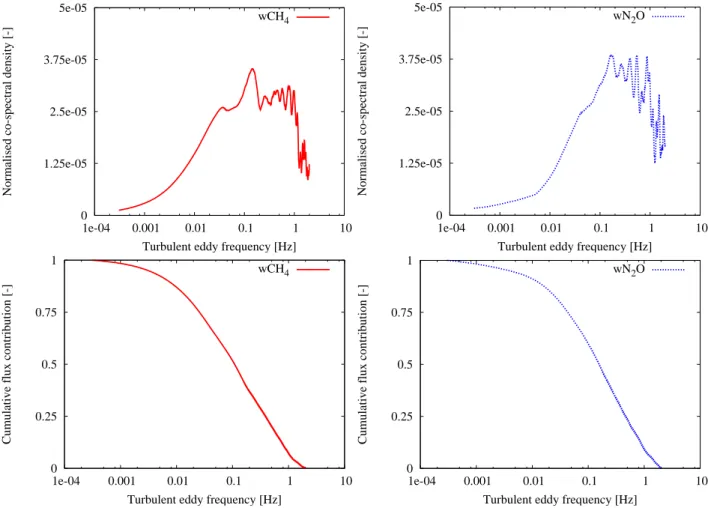
An estimate of the under- or overestimation was made by means of ogive analyses based on Lee et al. (2004). In this case, the ogives were determined by integrating the absolute normalized co-spectrum starting from the high frequencies. This ogive is defined by
OgwcF (fm)= (ns−1)1t 21t X i=m |Cowc(fi)| fi= i (ns− 1)1t; m = 1, 2, ..., h (ns− 1)1t 21t i . (10)
The absolute normalized co-spectra were calculated over one hour starting at 7 October 2006 12:00 and 13:00 for CH4
and N2O using block averaging. The average normalized
co-spectra were determined for each component over the two one-hourly co-spectra (Fig. 5). The amount of under- or over-estimation was derived using the OgwcF (8.3×10⁻³) in which
the frequency 8.3×10⁻³Hz corresponds to the used running mean time constant of 120 s (Fig. 5).
It was derived that the underestimation due to the 120 s running mean filter was 11% and 8% for CH4and N2O
dur-ing this period. Besides, it was checked if the average time of 30 min was long enough to include all the contributed ed-dies to the flux. This validation was done by comparing the
OgwcF values of the frequencies 3.0×10⁻⁴and 6.1×10⁻⁴Hz, which correspond to a time scale of 56 and 27 min, respec-tively. The difference was only 1%, therefore it was proved that an average time of 30 min was long enough in this case.
0 1.25e-05 2.5e-05 3.75e-05 5e-05 1e-04 0.001 0.01 0.1 1 10
Normalised co-spectral density [-]
Turbulent eddy frequency [Hz] wCH4 0 1.25e-05 2.5e-05 3.75e-05 5e-05 1e-04 0.001 0.01 0.1 1 10
Normalised co-spectral density [-]
Turbulent eddy frequency [Hz] wN2O 0 0.25 0.5 0.75 1 1e-04 0.001 0.01 0.1 1 10
Cumulative flux contribution [-]
Turbulent eddy frequency [Hz] wCH4 0 0.25 0.5 0.75 1 1e-04 0.001 0.01 0.1 1 10
Cumulative flux contribution [-]
Turbulent eddy frequency [Hz] wN2O
Fig. 5. The absolute normalized co-spectra and ogives with integration started from high frequencies of CH4flux (left) and N2O flux (right)
for determining the effect of the running mean filter and average time. The given ogives represent averages over 2 one-hourly measurements on 7 October 2006 between 12:00–14:00.
Although, more research should be done to derive the amount of underestimation due to the running mean and the minimal required average time for all circumstances.
Calibrations have to be performed to improve the accu-racy of the mixing ratio values and therefore the accuaccu-racy of the flux values. Three different correction factors were cal-culated a low, a high and a low-high calibration factor. The low-high calibration was defined by Eq. (2) and both other factors were determined by
fL= SL ML (11) fH= SH MH . (12)
The corrected concentration was found using one of these factors and the following equation
Ccor= fxCuncor (13)
with fx the low, high or low-high calibration factor, Cuncor
the uncorrected concentration value in ppb and Ccorthe
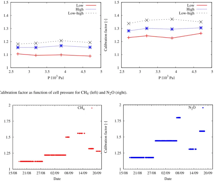
cor-rected concentration value in ppb. The low, high, and low-high calibration factors differ a lot (Fig. 6). This figure is based on an experiment with which the three calibration fac-tors are determined by different cell pressures. It can be seen that a single point calibration with one-standard can provide flux values that differ by up to 18% from a two-standard es-timate. By means of this, it can be stated that there will be a zero offset in our measurement system. Therefore, it will bet-ter to use a low-high calibration factor since the zero-offset should be the same for both. The lowest standard should be lower than the lowest expected atmospheric concentration and the highest standard should be higher than the highest expected concentration. Besides, the calibration factor will be more precise when more calibration standards are used. Only two standards are used in our case.
The calibration factor changed when instrument parame-ters were modified and when changes were made in fitting parameters or in alignment. The calibration factor seems to be slightly dependent on the cell pressure (Fig. 6). Therefore, it will be important to perform the calibrations at the pressure
1 1.1 1.2 1.3 1.4 1.5 2.5 3 3.5 4 4.5 5 Calibration factor [-] P [103 Pa] Low High Low-high 1 1.1 1.2 1.3 1.4 1.5 2.5 3 3.5 4 4.5 5 Calibration factor [-] P [103 Pa] Low High Low-high
Fig. 6. Calibration factor as function of cell pressure for CH4(left) and N2O (right).
1 1.25 1.5 1.75 2 15/08 21/08 27/08 02/09 08/09 14/09 20/09 Calibration factor [-] Date CH4 1 1.25 1.5 1.75 2 15/08 21/08 27/08 02/09 08/09 14/09 20/09 Calibration factor [-] Date N2O
Fig. 7. Calibration factor of CH4(left) and N2O (right) from 17 August to 22 September 2006. The cell pressure was nearly constant at
5.3×10³Pa (40 Torr) during this period.
of the measurements. The uncertainty in calibration factor will be a minor effect when a match of about 0.4×10³Pa is obtained. This match can easily be obtained. The calibra-tion factor is more dependent on the alignment and the fit-ting parameters. The maximal difference in calibration fac-tor was 0.44 and 0.63 for CH4and N2O, respectively, based
on data from 17 August until 22 September 2006 (Fig. 7). The cell pressure was nearly constant 5.3×10³Pa (40 Torr)
during this period. These calibration factors were based on manual calibrations which were performed each field visit. Automatic calibrations will be better, however, they could not be performed until now.
4.2 CH4and N2O exchange rates
4.2.1 Analysis using 30 min flux values
A dataset of CH4and N2O EC measurements was obtained
from 17 August to 6 November 2006 for which 99.8% was within the footprint of the investigated dairy farm site. About 7% of the CH4 and 22% of the N2O flux values were
re-jected by the instationarity tests (Foken and Wichura, 1996). The average standard deviations over six 5 min flux values were 84% and 185% for CH4and N2O, respectively. So, the
temporal variation was very large for both greenhouse gasses and especially for N2O. The accepted calibrated and
Webb-corrected 30 min NEE values are shown in Fig. 8.
In general the measurements for both CH4and N2O show
a net emission. About 98% and 91% of all flux values are positive for CH4 and N2O. In consequence, negative
-2500 0 2500 5000 15/08 29/08 12/09 26/09 10/10 24/10 07/11 Flux CH 4 [ngC m -2 s -1 ] Date CH4 -250 0 250 500 15/08 29/08 12/09 26/09 10/10 24/10 07/11 Flux N 2 O [ngN m -2s -1] Date N2O
Fig. 8. 30 min flux values of CH4(left) and N2O (right) from a dairy farm site in the Netherlands from 17 August to 6 November 2006.
-200 0 200 400 600 800 -60 -40 -20 0 20 40 60 Flux CH 4 [ngC m -2 s -1 ] Delay time [s] CH4 -50 0 50 100 150 200 -60 -40 -20 0 20 40 60 Flux N 2 O [ngN m -2 s -1 ] Delay time [s] N2O
Fig. 9. Correlation versus delay time plots for CH4(left) and N2O (right). The correlation plots represent averages over 4 half-hourly
measurements on 7 October 2006 between 12:00–14:00.
fluxes also occurred, however, the reliability should be an-alyzed in more detail to investigate if these fluxes were not caused by an instrumental artifact. Most fluxes were between
−1000 ngC m−2s−1 and 1000 ngC m−2s−1for CH4or
be-tween −100 ngN m−2s−1 and 100 ngN m−2s−1 for N2O.
The high positive peaks were clearly related to cow manure application. The negative fluxes occurred in short events last-ing at most a few hours. The negative CH4 fluxes mainly
occurred during low turbulence conditions with a friction ve-locity lower than 0.2 m s−1. This was not the case for the negative N2O fluxes. Therefore, most of the negative CH4
fluxes will be filtered when u*-filtering is applied.
The reliability of the negative fluxes was checked by a de-termination of the detection limit. The detection limit of the QCL spectrometer was derived using a method proposed by Wienhold et al. (1995). In this method, the standard devia-tion of the covariance funcdevia-tion far outside the true lag time
is used as the estimation. An example of a covariance func-tion is plotted in Fig. 9. The average detecfunc-tion limit of the QCL spectrometer was 41 ngC m−2s−1and 6 ngN m−2s−1 based on all 30 min flux values with a clear defined peak in the correlation plot. Thus, the estimated detection limit was probably most of the time much smaller than the measured CH4and N2O fluxes.
The conclusion is that large emissions of CH4and N2O
occurred at this dairy farm on peat grasslands. Moreover, negative emissions seemed to occur, however, more analy-ses should be performed to ascertain these uptakes. First, the raw data screening could be improved using an automatic screening based on the Vickers and Mahrt method (Vickers and Mahrt, 1997). Second, the negative fluxes should be an-alyzed using spectral analysis. For the net annual exchange, the uptake episodes were negligible.
0 500 1000 1500 34 35 36 37 38 39 40 41 42 43 44 0 50 100 150 Flux CH 4 [ngC m -2 s -1 ] Flux N 2 O [ngN m -2 s -1 ] Week number CH4 N2O 0 10 20 30 34 35 36 37 38 39 40 41 42 43 44 0 30 60 90 T [ 0 C] Rh [mm week -1 ] Week number Temperature Precipitation
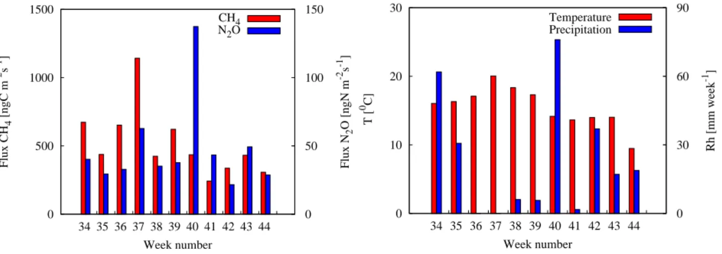
Fig. 10. Weekly average of CH4flux (left columns in red) and weekly average of N2O flux (right columns in blue) in left figure, and weekly
average of air temperature (left columns in red) and weekly precipitation rates (right columns in blue) in right figure measured at a dairy farm site in the Netherlands.
Table 2. Average and standard deviation of CH4 and N2O exchange at a dairy farm in the Netherlands over the period 17 August to 6
November 2006.
CH4[ngC m−2s−1] CH4[mg m−2hr−1] N2O [ngN m−2s−1] N2O [mg m−2hr−1]
NEE non-calibrated with Webb-correction 407±281 1.95±1.35 36±47 0.20±0.27
NEE calibrated with Webb-correction 512±385 2.46±1.85 52±69 0.29±0.39
4.2.2 Analysis using weekly flux values
Weekly average flux values were calculated when data cov-erage higher than 50% occurred in more than four days a week. An overview of weekly average CH4 flux and N2O
flux are presented in Fig. 10. The weekly average air tem-perature and the weekly precipitation rates are also shown in Fig. 10. These have been made available by KNMI in the Netherlands. Cow manure was applied in week 37. The high-est CH4weekly average flux also occurred in this week. The
highest N2O flux took place in week 40 after a large amount
of precipitation.
4.2.3 Analysis using three months of flux values
The average calibrated corrected NEE and the standard deviation in the average were 512±385 ngC m−2s−1 and 52±69 ngN m−2s−1from which 40% of N2O emission was
due to the fertilizing event. Thus, the standard deviations were of the same order of the average flux values, this was mainly caused by the fertilizing event The calibrated NEE was about 26% and 44% higher than the non-calibrated NEE for CH4and N2O, respectively.
The Webb-corrected NEE was 6% higher for CH4 and
34% higher for N2O than the non-Webb-corrected NEE.
The Webb-correction is probably somewhat lower since the correction is based on a near located open path system. However, the calibrated NEE values with Webb-correction seemed to be a good first estimation of the CH4 and N2O
exchange at this dairy farm on peat land since the overesti-mation of the Webb-correction is probably compensated by the underestimation due to the damping effect and the use of a running mean filter. A summary of non-calibrated Webb-corrected NEE and calibrated Webb-Webb-corrected NEE is given in Table 2.
5 Conclusions
A QCL was used for EC measurements of CH4and N2O.
Evaluation of its performance was performed using three months of continuous measurements at a dairy farm site on peat land in the Netherlands. The required criteria for eddy covariance flux measurements including continuity, sampling frequency, precision and stationarity were exam-ined. The system operated continuously from 17 August to 6 November 2006 with about one visit a week. The vali-dation of the sampling frequency of the system consisted of three parts, namely the electronic sampling frequency, the flow response and the damping. An electronic sampling
frequency of 10 Hz was obtained using a 1 GHz PC sys-tem. The flow response time was about 2 Hz and almost no damping to the flux contribution by the high frequency eddies occurred . Thus, the overall sampling frequency of the system was about 2 Hz. A precision of 2.9 ppb Hz−1/2 and 0.5 ppb Hz−1/2was obtained for CH4and N2O,
respec-tively. These values are close to the required precision val-ues of 4 ppb Hz−1/2and 0.3 ppb Hz−1/2. The precision was strongly dependent on the power on the detector and thus the alignment. The stationairity was checked using Allan vari-ance analyses and frequently calibration sessions. Drift in the system was removed using a 120 s running mean filter. A two-point calibration was required at least once a week.
The continuous operation of the system was also proven by three months of field measurements (data coverage of 87%). A first estimate of CH4and N2O exchange was made. The
average calibrated corrected exchange was 512 ngC m−2s−1 and 52 ngN m−2s−1 for CH4 and N2O, respectively, from
which 40% of N2O emission was due to the fertilizing event.
The N2O peak, which was strongly correlated to
precipita-tion, occured about three weeks after the fertilizing. Finally, although the dairy farm site was a net source of CH4 and
N2O, uptake also seemed to occur in short events lasting at
most a few hours. However, more research should be done to investigate the reliability of these negative fluxes.
In conclusion, a QCL spectrometer was suitable for per-forming continuous EC measurements of CH4 and N2O.
Nevertheless, a two-point calibration was necessary for ob-taining accurate estimates. Besides, the possible underesti-mation due to the damping effect, the use of a running mean filter and the limited effective sampling frequency should be analyzed in more detail.
Acknowledgements. This research was part of the Dutch National
Research Program BSIK ME1. Thanks are due to our colleagues P. van den Bulk, P. Fonteijn and T. Schrijver for their assistance during setting-up these experiments. We are also very grateful to E. Veenendaal of University of Wageningen for making available the latent heat flux data. Our thanks are also due to E. de Beus of Technical University of Delft for his assistance in data analyses. Finally, we owe a special debt of gratitude to the farmer T. van Eyk for using his farm site.
Edited by: A. Neftel
References
Allan, D. W.: Statistics of atomic frequency standards, Proceedings of the IEEE, 54, 221–230, 1966.
Ammann, C.: On the applicability of relaxed eddy accumulation and common methods for measuring trace gas surface fluxes, Diss. ETH No. 12795, Zurich, 1998.
Ammann, C., Brunner, A., Spirig, C., and Neftel, A.: Technical note: Water vapour concentration and flux measurements with PTR-MS, Atmos. Chem. Phys., 6, 4643–4651, 2006,
http://www.atmos-chem-phys.net/6/4643/2006/.
Eugster, W., Zeyer, K., Zeeman, M., Michna, P., Zingg, A., Buch-mann, N., and Emmenegger, L.: Nitrous oxide net exchange in a beech dominated mixed forest in Switzerland measured with a quantum cascade laser spectrometer, Biogeosciences Discuss., 4, 1167–1200, 2007,
http://www.biogeosciences-discuss.net/4/1167/2007/.
Faist, J., Capasso, F., Sivco, D. L., Sirtori, C., Hutchinson, A. L., and Cho, A. Y.: Quantum cascade laser, Science, 264, 553–556, 1994.
Foken, T. and Wichura, B.: Tools for quality assessment of surface-based flux measurements, Agr. Forest Meteorol., 78, 83–105, 1996.
Hargreaves, K. J., Fowler, D., Pitcairn, C. E. R., and Aurela, M.: Annual methane emission from Finnish mires estimated from eddy covariance campaign measurements, Theor. Appl. Clima-tol, 70, 203–213, 2001.
Hoogendoorn, C. J. and van der Meer, T. H.: Fysische trans-portverschijnselen II, Delftse Uitgevers Maatschappij, Delft, The Netherlands, 1991.
IPCC: Climate change 2001, The Scientific Basis, Cambridge Uni-versity Press, Cambridge, UK, 2001.
IPCC: Climate change 1995, Scientific and technical analyses of impacts, adaptations and mitigation. Contribution of working group II to the Second Assessment Report of the Intergovern-mental Panel on Climatic Change, Cambridge University Press, London, 2006.
Jim´enez, R., Herndon, S., Shorter, J. H., Nelson, D. D., McManus, J. B., and Zahniser, M. S.: Atmospheric trace gas measure-ments using a dual quantum-cascade laser mid-infrared absorp-tion spectrometer, Proceedings of SPIE, 5738, 318–331, 2005. Jonker, H. J. J., Duynkerke, P. G., and Cuijpers, J. W. M.:
Mesoscales fluctuations in scalars generated by boundary layer convection, J. Atmos. Sci., 56, 801–808, 1999.
Kaimal, J. C. and Finnigan, J. J.: Athmospheric boundary layer flows, Oxford University Press, Oxford, 1994.
Kormann, R. and Meixner, F. X.: An analytical footprint model for non-neutral stratisfication, Bound.-Lay. Meteorol., 99, 207–224, 2001.
Laville, P., Jambert, C., Cellier, P., and Delmas, R.: Nitrous oxide fluxes from a fertilized maize crop using micrometeorological and chamber methods, Agr. Forest Meteorol., 96, 19–38, 1999. Lee, X. L., Massman, W., and Law, B.: Handbook of
micromete-orology, Kluwer Academic Publishers, Dordrecht, The Nether-lands, 2004.
Lenschow, D. H. and Mann, J.: How long is long enough when measuring fluxes and other turbulent statistics?, J. Atmos. Ocean. Tech., 11, 661–673, 1994.
McMillen, R. T.: An eddy correlation technique with extended applicability to non-simple terrain, Bound.-Lay. Meteorol., 43, 231–245, 1988.
Monteith, J. L. and Unsworth, M. H.: Principles of environmental physics, Edward Arnold, London, 1990.
Neftel, A., Flechard, C., Ammann, C., Conen, F., Emmenegger, L., and Zeyer, K.: Experimental assessment of N2O background
fluxes in grassland systems, Tellus B, 59, 470–482, 2007. Nelson, D. D., Shorter, J. H., McManus, J. B., and Zahniser, M. S.:
Sub-part-per-billion detection of nitric oxide in air using a ther-moelectrically cooled mid-infrared quantum cascade laser spec-trometer, Appl. Phys. B, 75, 343–350, 2002.
Nelson, D. D., McManus, B., Urbanski, S., Herndon, S., and Zah-niser, M. S.: High precision measurements of atmospheric ni-trous oxide and methane using thermoelectrically cooled mid-infrared quantum cascade lasers and detectors, Spectrochimica Acta Part A, 60, 3325–3335, 2004.
Nieuwstadt, F. T. M.: Turbulentie, Epsilon Uitgaven Utrecht, Utrecht, The Netherlands, 1998.
Rothman, L. S. and Barbe, A.: The HITRAN molecular spectro-scopic database: edition of 2000 including updates through 2001, Journal of Quantitative Spectroscopy and Radiative Transfer, 82, 5–44, 2003.
Smith, K. A., Clayton, H., Arah, J. R. M., Christensen, S., Am-bus, P., Fowler, D., Hargreaves, K. J., Skiba, U., Harris, G. W., Wienhold, F. G., Klemedtsson, L., and Galle, B.: Micrometeoro-logical and chamber methods for measurement of nitrous oxide fluxes between soils and the atmosphere: Overview and conclu-sions, J. Geophys. Res., 99, 16 541–16 548, 1994.
Veenendaal, E. M., Kolle, O., Leffelaar, P., Schrier-Uijl, A. P., van Huissteden, J., van Walsem, J., M¨oller, F., and Berendse, F.: Land use dependent CO2exchange and carbon balance in two
grassland sites on eutropic drained peat soils, Biogeosciences Discuss., 4, 1633–1671, 2007,
http://www.biogeosciences-discuss.net/4/1633/2007/.
Vickers, D. and Mahrt, L.: Quality control and flux sampling prob-lems for tower and aircraft data, J. Atmos. Ocean. Tech., 14, 512– 526, 1997.
Webb, E. K., Pearman, G. I., and Leuning, R.: Correction of flux measurements for density effects due to heat and water vapour transfer, Q. J. Roy. Meteor. Soc., 106, 85–100, 1980.
Werle, P. and Kormann, R.: Fast chemical sensor for eddy-correlation measurements of methane emissions from rice paddy fields, Appl. Opt., 40, 846–858, 2001.
Werle, P. and Slemr, F.: Signal-to-noise ratio analysis in laser ab-sorption spectrometers using optical multipass cells, Appl. Opt., 30, 430–434, 1991.
Wienhold, F. G., Frahm, H., and Harris, G. W.: Measurements of N2O fluxes from fertilized grassland using a fast response
tunable diode laser spectrometer, J. Geophys. Res., 99, 16 557– 16 567, 1994.
Wienhold, F. G., Welling, M., and Harris, G. W.: Micrometeoro-logical measurement and source region analysis of nitrous oxide fluxes from an agricultural soil, Atmos. Environ., 29, 2219–2227, 1995.