HAL Id: hal-00331149
https://hal.archives-ouvertes.fr/hal-00331149
Submitted on 15 Oct 2008
HAL is a multi-disciplinary open access
archive for the deposit and dissemination of
sci-entific research documents, whether they are
pub-lished or not. The documents may come from
teaching and research institutions in France or
abroad, or from public or private research centers.
L’archive ouverte pluridisciplinaire HAL, est
destinée au dépôt et à la diffusion de documents
scientifiques de niveau recherche, publiés ou non,
émanant des établissements d’enseignement et de
recherche français ou étrangers, des laboratoires
publics ou privés.
the northwestern Mediterranean Sea
E. Praca, A. Gannier
To cite this version:
E. Praca, A. Gannier. Ecological niches of three teuthophageous odontocetes in the northwestern
Mediterranean Sea. Ocean Science, European Geosciences Union, 2008, 4 (1), pp.49-59. �hal-00331149�
www.ocean-sci.net/4/49/2008/
© Author(s) 2008. This work is distributed under the Creative Commons Attribution 3.0 License.
Ocean Science
Ecological niches of three teuthophageous odontocetes in the
northwestern Mediterranean Sea
E. Praca1,2and A. Gannier3
1Centre de Recherche sur les C´etac´es – Marineland, Antibes, France
2MARE Center – Laboratory for Oceanology, University of Li`ege, Li`ege, Belgium 3Groupe de Recherche sur les C´etac´es, Antibes, France
Received: 23 August 2007 – Published in Ocean Sci. Discuss.: 10 October 2007 Revised: 20 December 2007 – Accepted: 9 January 2008 – Published: 7 February 2008
Abstract. In the northwestern Mediterranean Sea, sperm whales, pilot whales and Risso’s dolphins prey exclusively or preferentially on cephalopods. In order to evaluate their competition, we modelled their habitat suitability with the Ecological Niche Factor Analysis (ENFA) and compared their ecological niches using a discriminant analysis. We used a long term (1995–2005) small boat data set, with vi-sual and acoustic (sperm whale) detections. Risso’s dolphin had the shallowest and the more spatially restricted principal habitat, mainly located on the upper part of the continental slope (640 m mean depth). With a wider principal habitat, at 1750 m depth in average, the sperm whale used a deeper part of the slope as well as the closest offshore waters. Fi-nally, the pilot whale has the most oceanic habitat (2500 m mean depth) mainly located in the central Ligurian Sea and Provenc¸al basin. Therefore, potential competition for food between these species may be reduced by the differentiation of their habitats.
1 Introduction
The ecological niche of a species is a complex set of variables characterized by three principal axes: habitat (influence of environmental factors defining the spatial distribution), diet (prey species, trophic level) and seasonality (use of resources and space according to time) (L´evˆeque, 2001; Frontier and Pichod-Viale, 1998). Theoretically, each species has its own ecological niche. Two species sharing close niches, i.e. the same prey species and distribution area, will be in competi-tion. The less efficient species in exploiting these resources
Correspondence to: E. Praca
will be partially or totally excluded from the area (L´evˆeque, 2001; Frontier and Pichod-Viale, 1998). Otherwise, special-ization of both species will occur with emergence of different seasonality, and/or with a specialization or a diversification of the diet (Whitehead et al., 2003).
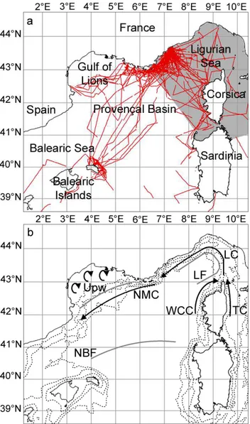
In the northwestern Mediterranean Sea (NWMS) (Fig. 1a), the sperm whale (Physeter macrocephalus), the long-finned pilot whale (Globicephala melas), Risso’s dolphin (Grampus
griseus) and Cuvier’s beaked whale (Ziphius cavirostris) are
teuthophageous, i.e. they prey exclusively or preferentially on cephalopods (Astruc and Beaubrun, 2005). The three for-mer species have been shown to be common over the whole study area, while the latter displays a more restricted distri-bution (Gannier, 1999; Azzellino et al., 2003; Podesta et al., 2006). Our surveys covered most of the NWMS (Fig. 1a) and resulted in only three observations of Cuvier’s beaked whale. Consequently, our work did not deal with this species.
The stomach contents of stranded animals in the Mediter-ranean show an overlap of the diet of sperm whales, pilot whales and Risso’s dolphins. Their principal prey are a few species of bathypelagic cephalopods of the Histioteuthidae and Ommastrephidae families (Astruc and Beaubrun, 2005). Furthermore, previous studies highlighted similar trends in their distribution. The sperm whale, the most studied species, seems to be opportunistic in its habitat use, exploiting ar-eas with steep slopes, as well as offshore waters featuring SST fronts (Gannier and Praca, 2007; Gannier et al., 2002). Risso’s dolphin seems to prefer waters with steep slopes from 500 to 2000 m (Bompar, 1997; Gannier, 1998b), while the pilot whale might prefer more oceanic areas, with waters deeper than 1000 m (Gannier, 1998b). However, the studies on Risso’s dolphins and pilot whales were principally con-ducted in the Ligurian Sea and/or in the Gulf of Lions and did not cover the entire NWMS.
Fig. 1. The northwestern Mediterranean Sea. (a) Main basins, the
International Sanctuary for Marine Mammals, Pelagos (grey area) and the effort realised during surveys in summer from 1995 to 2005 (red lines); (b) Topographic and oceanographic features: 200 m, 1000 m and 2000 m contours (dashed lines), upwellings (Upw), currents (black arrows: WCC – Western Corsican Current, TC – Tyrrhenian Current, LC – Ligurian Current, NMC – North Mediter-ranean Current) and fronts (grey lines: LF – Ligurian Front, NBF – North Balearic Front).
As possible competition between these species may oc-cur, it was interesting to improve knowledge of their ecolog-ical niches and in particular of their habitats. The present study focuses on the influence of environmental factors, in the whole northwestern basin and for a ten year time scale. We modelled the three species’ habitat suitability with the Ecological Niche Factor Analysis and compared their niches with a discriminant analysis.
2 Material and methods 2.1 Study area
The NWMS (between 2.5◦E and 9.5◦E, 39.5◦N and 44.5◦N) has complex topographic and oceanographic fea-tures (Fig. 1b). Both steep and narrow slopes (Provence, Balearic and north-eastern Corsican coasts) and large smooth continental shelves (Gulf of Lions, western Sardinian coast) are encountered (Biju-Duval and Savoye, 2001). The to-pography and wind regime lead to a cyclonic circulation of modified Atlantic waters from the Ligurian to the Balearic Sea. The Ligurian front (LF) and the North Balearic front (NBF) are permanent, seasonally fluctuating fronts. By con-trast, the presence of fronts between waters of the North-Mediterranean current (NMC) and cold upwelled waters from the Gulf of Lions depends on the occurrence of Mis-tral and Tramontane winds (Lopez-Garcia et al., 1994; Mil-lot, 1999; Millot and Wald, 1990; Le Vourch et al., 1992). Although an oligotrophic basin, and generally unproduc-tive, the NWMS features an important phytoplankton bloom with chlorophyll concentrations peaking between 0.8 and 2.5 mg m−3, usually occurring in March (Morel and Andr´e, 1991). In the Gulf of Lions, the Rhˆone river exports high quantities of nutrients and particles (Conan et al., 1998), which increase the turbidity. This phenomenon leads to an overestimation of chlorophyll concentrations in satellite data (>0.8 mg m−3even in summer) and the Rhˆone panache can be classified as turbid case 2 water (Antoine et al., 1996). Consequently, the area influenced by the panache of the Rhˆone was removed from our analysis.
2.2 Data collection and standardisation
Dedicated surveys were conducted on a motor-sailing boat every summer from 1995 to 2005. The protocol combined visual searching and systematic discrete acoustic sampling (for details see Gannier, 1998a; Gannier et al., 2002). In brief, the visual searching was conducted by three observers scanning continuously with naked eyes, from abeam forward on both sides of the vessel. The acoustical sampling used a towed hydrophone and consisted of listening for 1 min ev-ery 2 nm (3.7 km) along the cruise track. Sperm whales were recognized by their typical signal composed of regular clicks (Teloni, 2005). For pilot whales and Risso’s dolphins, only visual detections were used. Their acoustic signals could be confused with each other and with other delphinids. For each listening or visual sighting, we recorded sea state, position of the boat and of the cetaceans, visual conditions (V , ing between 0 and 6), background acoustic noise (U , vary-ing between 1 and 5) and the bio-acoustic signal levels (SL, varying between 0 and 5). V , U and SL were subjectively estimated by experienced observers. Data with V <4, U >3 or SL<2 were removed from the data set.
In order to avoid autocorrelation in the analysis, data were merged into observation sequences in ArcGIS 8.3©. For sperm whales, all acoustical or visual successive observa-tions obtained without a minimum of one hour time-lag be-tween them were considered to be from the same animal or group (Gordon et al., 2000). For positioning the observation sequence, we chose either the location of a visual sighting or of the acoustic detection with the best SL. For pilot whales and Risso’s dolphins, the location of the first visual sighting was chosen.
The Eco-Geographical Variables (EGVs) were classical data used in cetacean habitat modelling (e.g. Hamazaki, 2002), related to topography, temperature, salinity and pri-mary production. Depth was obtained from the GEBCO© Digital Atlas (IOC-IHO-BODC, 2003). It was used to calcu-late the slope and the distance to the 200 m contour, which was shown to be more relevant than the coastline contour for these species (Mangion and Gannier, 2002). Sea Sur-face Temperature (SST) data were downloaded, depending on their availability, from the websites of the Pathfinder sor for 1995 to 2002 data (PO.DAAC) and of the Modis sen-sor for 2002 to 2005 data (OceanColor). The front detec-tion maps were computed on the basis of SST maps using a Sobel filter available in Idrisi Andes©. Salinity data from 1889 to 2002 were obtained from the MEDAR/MEDATLAS II database (MODB) and chlorophyll concentration data for the 1998 to 2005 period from the SeaWifs sensor website (OceanColor).
For the hydrological and biological EGVs, we used monthly maps to compute average situations for two periods: the summer (June, July and August) and the phytoplankton bloom period (February, March and April). These yearly sea-sonal maps were then averaged over all years of the survey period, resulting in two seasonal maps for each EGV. Salin-ity and chlorophyll concentration were not available for all years, but available data overlapped 80% of the survey period and were considered to be representative of average condi-tions.
The study area was modelled as a 9*9 km grid cell in Idrisi Andes© and both species presence and EGV grids were com-puted using it. This resolution was chosen to correspond with the available monthly chlorophyll concentration data. 2.3 Habitat modelling
Classical habitat modelling techniques (e.g. Generalised Lin-ear Model – GLM or Generalised Additive Model – GAM) are based on presence-absence data (Guisan and Zimmer-mann, 2001; Redfern et al., 2006). “True” absence data (when animals are actually absent) are not easy to collect for mobile or inconspicuous species such as cetaceans which are able to spend long periods underwater. Biases may be caused by “false” absence data, when animals are present but not detected. For pilot whales and Risso’s dolphins, such
biases could not be avoided by the use of acoustic data col-lected along the survey track, as they were for sperm whales. Furthermore, this method was not applicable because of the smaller data sets for these two species. The goal of this work was to compare the habitats of three species, using a method that can be implemented for each species’ data set. We therefore choose to use a new presence-only method: the Ecological-Niche Factor Analysis (ENFA) (Hirzel et al., 2002).
A detailed description of the ENFA and its mathematical computations are given in Hirzel et al. (2002, 2006b). The ENFA is a presence-only multifactorial analysis, comparing the distribution of species to the global available environment in the hyperspace defined by the EGVs. The transformation of EGVs into a set of uncorrelated factorial axes introduces ecological significance. Marginality (how much a species’ habitat differs from the mean available conditions) is repre-sented in the first factorial axis and specialization (breadth of the ecological niche) is maximised in the subsequent axes. The factorial axes’ coefficients give the importance of each EGV in the different axes and the relative range of the EGVs preferred by the species. They are also used to compute global marginality (M, varying generally between 0 and 1) and specialization (S, indicating some degree of specializa-tion when greater than 1). Finally, a Habitat Suitability (HS) map is built with the median algorithm. It compares the posi-tion of each cell of the study area to the distribuposi-tion of pres-ence cells on the different factorial axes. HS values range from 0 to 100: a cell adjacent to the median of an axis would score 100 and a cell outside of the species distribution would score zero. All the ENFA analyses were conducted using Biomapper 3.2© software (Hirzel et al., 2006a).
2.4 Model validation
The evaluation of a model incorporates both the evaluation of its statistical accuracy and the ecological meaning when compared to previous studies on the species’ distribution. A “good” model should be statistically significant and coherent to what is known on the ecology of the species studied. As we used a presence-only modelling technique, the classical study of the confusion matrix (counting how many presence and absence validation cells occur in predicted suitable and unsuitable areas) was not possible. The model validation was therefore achieved with a k-fold cross-validation (Boyce et al., 2002; Hirzel et al., 2006b; Fielding and Bell, 1997), as explained below.
The model is evaluated by the trend of the predicted-to-expected ratio curve (p/e curve) and the continuous Boyce index (B) (Hirzel et al., 2006b). A perfect model would have a strait increasing line p/e curve. B is a Spearman rank cor-relation between Fi (predicted-to-expected ratio) and the HS
values. It varies between −1 and 1, a perfect model having a B=1. However, Hirzel et al. (2006b) compared the accu-racy of different validation methods and found that a B≈0.6
Table 1. Continuous Boyce index (B, varying between −1 and 1),
global marginality (M, varying generally between 0 and 1) and spe-cialization (S, indicating some degree of spespe-cialization when supe-rior to 1) for the sperm whale, the pilot whale and Risso’s dolphin.
Species B (mean±SD) M S
sperm whale 0.61±0.50 0.77 1.40
pilot whale 0.58±0.19 0.85 3.31
Risso’s dolphin 0.39±0.21 1.03 1.89
corresponds to an Area Under the Receiver Operating Char-acteristic (ROC) curve >0.9 (ROC evaluates the proportion of correctly and incorrectly classified predictions over a con-tinuous range of presence-absence thresholds. The closer the Area Under the Curve is to 1, the more the model fits well. See Boyce et al. (2002) for details).
In practice, the presence data set is partitioned into k in-dependent subsets, and k−1 partitions are used in the cali-bration data set, leaving the last partition as the validation data set. The number of partitions k was chosen following Huberty’s rule for the pilot whale (k=4) and Risso’s dolphin (k=3) (Fielding and Bell, 1997). For the sperm whale, k was fixed at 10, which seems to be the best number of partitions when there are more than 100 cells with observed presence (Hirzel et al., 2006a).
The predicted-to-expected ratio Fi is calculated as:
Fi = Pi Ei (1) Pi = Oi P Oi (2) Ei = Ai P Ai (3) In Eqs. (1), (2) and (3), Pi is the predicted frequency of
eval-uation cells, with Oi the number of presence validation cells
falling in an HS window i and POi the total number of
presence validation cells. Ei is the expected frequency of
evaluation cells, with Aithe number of all cells belonging to
the same HS window i andPAithe total number of cells in
the whole study area.
We define an HS window as a range of HS values with a constant span of 20 units. Fi is first computed in the HS
win-dow ranging from zero to 20 units ([0; 20]). The winwin-dow is then shifted upward one HS unit and Fi is computed again.
This operation is repeated until the moving window reaches the last possible range [80; 100]. It provides the p/e curve, which plots Fi against the HS values. For a random model,
Fi is equal to one for every window i. If a model
prop-erly predicted the suitable areas of one species, then Fi<1
in windows with low HS values and Fi>1 for windows with
high HS values, and it features a monotonically increasing
p/e curve. B is then computed between Fi and the average
HS values of the different windows. The p/e curves and B are produced k times, each time leaving out another valida-tion partivalida-tion, allowing the assessment of their central trend and variance (here we present the mean ±SD). Using the p/e curve, a threshold between unsuitable and suitable areas was estimated following Hirzel et al. (2006b), and is the point where Fi becomes clearly >1 and from which the p/e curve
stops to oscillate around this limit. This permits us to de-termine a suitable area for each species and to compute its environmental characteristics.
2.5 Niche differentiation
In addition to the habitat suitability models, a discriminant analysis was undertaken to compare the ecological niches of the sperm whale, the pilot whale and Risso’s dolphin (Leg-endre and Leg(Leg-endre, 1998). This technique is a multivari-ate analysis using the space defined by the EGVs and the species’ distributions simultaneously. It computes discrimi-nant factors that maximise the interspecific variance and min-imize the intraspecific variance. In Biomapper 3.2©, the dis-criminant factors are used to compute indices quantifying the niches’ breadth and overlap. The Hurlbert index (B′)
mea-sures the breadth of the niches. It varies between 0 (corre-sponding to specialized species) and 1 (corre(corre-sponding to gen-eralist species) (Hurlbert, 1978). Lloyd’s asymmetric overlap index (Z) evaluates the overlapping of species niches two by two. Zx(y)is the part of the niche of X, which is also shared
by Y . In other words, it is the overlapping of the niche of Y on the niche of X (Hurlbert, 1978).
3 Results
3.1 Habitat suitability models
All global marginality, specialization and Boyce indices are presented in Table 1. Boyce indices decreased with the number of presence cells from 0.61 for the sperm whale to 0.39 for Risso’s dolphin. All three species displayed a high marginality, from 0.77 to 1.11, but specialization coefficients were more variable (from 1.40 to 3.31).
3.1.1 Sperm whale
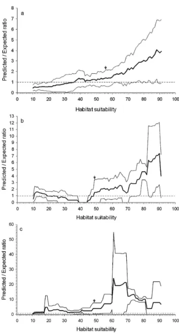
The total number of presence cells was 175 for the sperm whale. The model of this species was highly fitted as shown by a B=0.61±0.50 and a quasi-monotonic p/e curve (Fig. 2a). This species had an overall marginality of 0.77 and an overall specialization of 1.40, indicating that its habitat is different from the mean environment available, but still quite wide.
The marginality factorial axis indicated a strong relation-ship for cells with a steep slope (coefficients of 0.49) and close to the 200 m contour (−0.42). This axis also showed
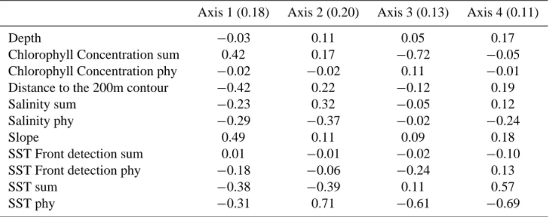
the importance of high chlorophyll concentrations in summer (0.42) and low SST for summer (−0.38) and for the phyto-plankton bloom period (−0.31). Specialization axes high-lighted the restriction of the species to the lower SST (co-efficients varying between 0.61 and 0.71 in spring), lower salinity (0.32 for the summer and 0.37 for the phytoplankton bloom period) and higher chlorophyll concentrations (0.72 in summer). Bottom depth did not seem to be an important variable for this species (Table 2). The suitable area cor-responded to HS values greater than 56 and showed a core habitat on the continental slope of the whole area, including the Balearic and Corsica islands, and in closer offshore wa-ters (Fig. 3a). The characteristics of the suitable area of this species were: mean depth of 1748 m, mean slope of 2.1◦and mean summer SST of 21.9◦C.
3.1.2 Pilot whale
The total number of presence cells for the pilot whale was 33. This model had a B of 0.58±0.19 i.e. a well fitted model. Its p/e curve increased quasi-monotonically between 39 and 90 HS values, but decreased between 0 and 39, and between 90 and 100 (Fig. 2b). The strong global marginality of 0.85 and the high total specialization of 3.31 indicated that pilot whales have a restricted habitat in comparison with the mean environment of the study area.
Both marginality and specialization axes highlighted a strong relationship with the colder SST for summer (marginality of −0.57 and specialization of 0.42) and phyto-plankton bloom period (−0.49 for the marginality, 0.42 and 0.82 for the specialization), and higher chlorophyll concen-trations in summer (marginality of 0.51 and specialization of 0.77). The first specialization axis also showed a restric-tion to deep waters (coefficient of 0.37) (Table 3). For this species, the threshold between unsuitable and suitable areas was estimated to the HS value of 49. This highlighted a prin-cipal habitat in oceanic waters of the central Ligurian Sea and Provenc¸al basin (Fig. 3b). This species preferred an area with a mean depth of 2511 m, a mean slope of 0.55◦and a
mean summer SST of 21.7◦C.
3.1.3 Risso’s dolphin
The total number of presence cells for Risso’s dolphin was 23. The ENFA typically requires a number of EGVs less than 1/2 to 1/3 of the number of presence cells (Alexandre Hirzel, pers. comm.), which limits the number of EGVs for this species. We therefore carried out a step-by-step descend-ing exclusion of the EGVs and chose the model with the best validation.
The model for Risso’s dolphin was less meaningful than for the two other species, with a B=0.39±0.21 and a more variable p/e curve.
The marginality axis indicated a strong relationship with a steep slope (coefficient of 0.64), short distance to the
Fig. 2. Predicted-to-expected ratio curve (mean±SD) and threshold
between unsuitable and suitable areas (arrow) for (a) sperm whale,
(b) pilot whale and (c) Risso’s dolphin models (the limit of random
models, predicted-to-expected ratio Fi=1, is indicated by the dotted
line).
200 m contour (−0.63) and a certain affinity for shallow areas (depth coefficient of −0.30). The affinity for cells close to the 200 m contour was important in each specialization axis (coefficients from 0.43 to 0.61). These axes also indicated an affinity for higher chlorophyll concentrations in summer (0.77) and steeper slopes (0.73) (Table 4).
The suitable area for Risso’s dolphin corresponded to HS values above 49 (Fig. 2c). Due to a very high marginality >1 and an important specialization (1.89), the principal habitat of this species was restricted. It was located on the upper part
Table 2. Relevant axes (with their eigenvalues) and the EGV coefficients of the sperm whale model (sum: summer period, i.e. June, July
and August; phy: phytoplankton bloom period, i.e. February, March and April). The positive or negative sign is relevant for the first axis coefficients, but in the following axes only the absolute value of coefficients is considered.
Axis 1 (0.18) Axis 2 (0.20) Axis 3 (0.13) Axis 4 (0.11)
Depth −0.03 0.11 0.05 0.17
Chlorophyll Concentration sum 0.42 0.17 −0.72 −0.05
Chlorophyll Concentration phy −0.02 −0.02 0.11 −0.01
Distance to the 200m contour −0.42 0.22 −0.12 0.19
Salinity sum −0.23 0.32 −0.05 0.12
Salinity phy −0.29 −0.37 −0.02 −0.24
Slope 0.49 0.11 0.09 0.18
SST Front detection sum 0.01 −0.01 −0.02 −0.10
SST Front detection phy −0.18 −0.06 −0.24 0.13
SST sum −0.38 −0.39 0.11 0.57
SST phy −0.31 0.71 −0.61 −0.69
Table 3. Relevant axes (with their eigenvalues) and the EGV coefficients of the pilot whale model (sum: summer period, i.e. June, July
and August; phy: phytoplankton bloom period, i.e. February, March and April). The positive or negative sign is relevant for the first axis coefficients, but in the following axes only the absolute value of coefficients is considered.
Axis 1 (0.33) Axis 2 (0.31) Axis 3 (0.15)
Depth 0.18 −0.37 −0.03
Chlorophyll Concentration sum 0.51 0.77 −0.30
Chlorophyll Concentration phy 0.16 −0.14 −0.03
Distance to the 200m contour −0.09 0.06 −0.05
Salinity sum 0.01 −0.06 −0.18
Salinity phy −0.01 0.14 0.12
Slope 0.22 −0.20 −0.07
SST Front detection sum 0.01 0.03 0.03
SST Front detection phy −0.24 0.04 −0.07
SST sum −0.57 0.07 0.42
SST phy −0.49 0.42 −0.82
Table 4. Relevant axes (with their eigenvalues) and the EGV coefficients of Risso’s dolphin model (sum: summer period, i.e. June, July
and August; phy: phytoplankton bloom period, i.e. February, March and April). The positive or negative sign is relevant for the first axis coefficients, but in the following axes only the absolute value of coefficients is considered.
Axis 1 (0.46) Axis 2 (0.25) Axis 3 (0.17) Axis 4 (0.08)
Depth −0.30 −0.16 −0.09 −0.44
Chlorophyll Concentration sum 0.26 0.77 0.29 0.28
Distance to the 200m contour −0.63 0.48 −0.61 0.43
Salinity sum −0.14 −0.01 0.05 −0.45
Slope 0.64 0.18 −0.73 0.15
Fig. 3. Habitat suitability maps for (a) sperm whale, (b) pilot whale
and (c) Risso’s dolphin models (the grey area was removed from the analysis). Black dots represent the location of presence cells used in the model of each species.
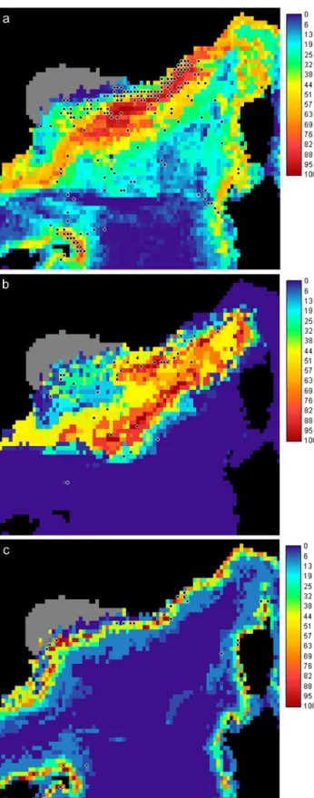
Fig. 4. Distribution of cells of the study area and of observations of
the sperm whale, the pilot whale and Risso’s dolphin along the first discriminant factor.
of the continental slope of the whole study area (Fig. 3c), with mean characteristics of: 638 m for the depth, 3.6◦for
the slope and 22.2◦C for the summer SST.
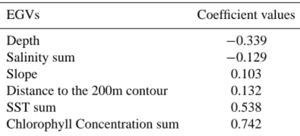
3.2 Niche differentiation between the three species For the discriminant analysis, we limited the number of EGVs to those highlighted as important by the ENFA. The first and second discriminant factors had eigenvalues of 36.53 and 12.49 respectively, showing that they discrimi-nated between the species niches very well. As the two discriminant factors highlighted the same trends and as the eigenvalue of the first factor was three times higher than that of the second, we only used the first. The distribution ranges of species observations along the axis showed that habitats of Risso’s dolphins and pilot whales were well separated, while that of sperm whales was more extended and overlapped the two others (Fig. 4). EGVs with positives values seemed to favour Risso’s dolphin and showed a more coastal habitat, with the influence of an important slope, relatively warm waters with high chlorophyll concentrations and a short dis-tance to the 200m contour (Table 5). On the contrary, the observations of pilot whales were linked to EGVs with neg-ative values and highlighted an offshore habitat with greater depth and relatively high salinity (Table 5). The distribution of sperm whale observations had a principal peak in the neg-ative values, but there were numerous observations with pos-itive values as well. The discriminant analysis was not able to highlight a particular trend for the habitat of this species.
The Hurlbert’s niche breath index indicated that the sperm whale had the wider niche (B′=0.62), followed by the
pi-lot whale (B′=0.55) and Risso’s dolphin that seemed very
specialized for its habitat (B′=0.02). Lloyd’s asymmetric
overlap indices (Table 6) confirmed that the sperm whale niche overlapped an important part of both niches of the pilot whale and Risso’s dolphin (respectively Z=18.45 and 3.00), while the reciprocal overlaps were small (Z=3.47 for the pi-lot whale and Z=0.37 for Risso’s dolphin). Furthermore,
Table 5. Coefficients of the EGVs along the first discriminant factor
(sum: summer period, i.e. June, July and August; phy: phytoplank-ton bloom period, i.e. February, March and April).
EGVs Coefficient values
Depth −0.339
Salinity sum −0.129
Slope 0.103
Distance to the 200m contour 0.132
SST sum 0.538
Chlorophyll Concentration sum 0.742
the niche overlap indices of pilot whales and Risso’s dolphin were nil, meaning their niches were totally separated.
4 Discussion and conclusion 4.1 Model evaluation
ENFA produced meaningful habitat predictions for three species with variable amounts of presence data: using 175 cells of presence for the sperm whale and 33 for the pi-lot whale, we obtained well fitted models. For Risso’s dol-phin, the validation was less satisfactory, probably as a con-sequence of the limited number of presence cells of this species. Nevertheless, the HS map produced for this species is in general agreement with studies on its distribution (Gan-nier, 1998b; Azzelino et al., 2001). While GLM or GAM seem to be more accurate than ENFA (e.g. Brotons et al., 2004), this later is a useful tool when absence data are not reliable enough, or when species are rare. As suggested by our results, this method seemed to be quite robust to model a first attempt to estimate the suitability of an area with a small data set.
The habitats highlighted here were not strictly feeding grounds. Indeed, the visual observations used, in particu-lar for pilot whales and Risso’s dolphins, did not concern only feeding behaviour. The use of passive acoustic or tags suggested that sperm whales feed during the day (Drouot et al., 2004; Watwood et al., 2006), while pilot whales seem to be predominantly night feeders (Baird et al., 2002). The daily feeding pattern of Risso’s dolphin is still unclear, but this species seems to be a night feeder too (Gannier, unpub-lished data). Pilot whales and Risso’s dolphins often seem to rest and socialize during daytime. Nevertheless, at the spatial scale of our models, it is an acceptable assumption that they are close to the locations where they feed during the night.
The use of data compiled and averaged over a large spatial and temporal scale seemed to attenuate the accuracy of our models in some areas. For example, Gannier (1998b) found that sperm whales could have a deeper habitat, using only the observations done in the Ligurian sea. Similarly, Gannier
Table 6. Lloyd’s asymmetrical overlap indices (Zx(y)) between the
niches of the sperm whale, the pilot whale and Risso’s dolphin.
Y
X sperm whale pilot whale Risso’s dolphin
sperm whale – 3.47 0.38
pilot whale 18.42 – 0.00
Risso’s dolphin 3.00 0.00 –
and Praca (2007) showed that thermal fronts, and in particu-lar the North Balearic front (NBF), seemed to be favourable to sperm whales. However, they used smaller spatial and temporal scales (depths greater than 2000 m and a weekly time scale respectively).
There is still a difference of effort between continental slope areas and offshore waters. This difference is due to the difficulty of surveying offshore waters in relation to the autonomy of the boat used and to the availability of good weather conditions during extended periods. The distribu-tion of cetaceans in offshore waters will only be clarified with more survey effort in those areas.
The possibility of weighting the presence data with the ef-fort was considered during the modelling process. For the pilot whale and Risso’s dolphin, it introduced more bias than having no weighting in relation to the small size of the data set. For the sperm whale, it did not highlight the potential offshore habitat and only decreased the statistical accuracy of the model. This weighting was therefore not used. However, sperm whales seemed to be influenced by both topographical and hydrological variables. The continental slope is a fixed spatial variable where observations of sperm whales are more concentrated. On the contrary, movements of fronts, such as the NBF, lead to a spatial spread of observations of sperm whales. Even if we could use frontal characteristics synchro-nized with sperm whales’ positions, the consequence of hav-ing a NBF movhav-ing over the years would be an “unfocused” spatial picture of the offshore habitat.
As we pooled variables over a ten year period, the ef-fect of inter-annual variations on our models was trouble-some. Little is known about cephalopods’ spatial distribution and movements at a large scale in the NWMS, but they are susceptible to following their prey and being influenced by inter-annual changes. Teuthophageous cetaceans certainly have the ability to detect and track moving prey. For ex-ample, their echolocation pulses can be heard several kilo-metres away (delphinids) or more (sperm whales) (Drouot et al., 2004). Successful feeding by individuals or groups can be consequently detected by conspecifics in the surround-ing areas. From place to place, this “eavesdroppsurround-ing“ effect might help to concentrate these predators in the locations where the prey availability is higher. However, our modelling
strategy was to attempt a global description in a temporally and spatially heterogeneous area, the entire NWMS, instead of modelling the habitat in restricted and more homogeneous regions, as proposed by Ca˜nadas et al. (2002) for odonto-cetes or Panigada et al. (2005) for fin whales (Balaenoptera
physalus). The influence of inter-annual variations of
envi-ronmental variables should be studied at a smaller scale. 4.2 Comparison of the ecological niches
The summer habitat niches of pilot whales, Risso’s dolphins and sperm whales seemed to be segregated and differ in their habitat characteristics. The pilot whale presented the most oceanic habitat with a strong relationship with the lowest SST, the highest chlorophyll concentrations and depth of the study area. Risso’s dolphin has the shallowest habitat, on the upper part of the slope, and is mainly influenced by the proximity of the 200 m contour. The sperm whale has the wider habitat, over the entire continental slope, and slightly offshore, and seems to be influenced by both topographical and hydrological factors.
In the Alboran Sea, southwestern Mediterranean, the three species seem to have closer habitats. Risso’s dolphin and the long-finned pilot whale are found in waters deeper than 600 m and the sperm whale in waters deeper than 700 m (Ca˜nadas et al., 2002; Ca˜nadas et al., 2005). Regarding the slope, the most influenced species seems to be Risso’s dol-phin which preferred slopes greater than 40 m km−1(2.29◦), followed by the pilot whale (between 20 and 80 m km−1, i.e. 1.15 and 4.58◦) and the sperm whale which did not show any preference (Ca˜nadas et al., 2002). In the Gulf of Mexico, a tropical area, the preferred depths of the sperm whale, Risso’s dolphin and the short-finned pilot whale
(Glo-bicephala macrorhynchus) are close to those found in the
Alboran Sea (Baumgartner et al., 2001; Davis et al., 1998). Risso’s dolphin seems to have similar habitats in the Alboran Sea, Gulf of Mexico and NWMS. For the sperm whale, dif-ferences appear for the slope, which seems to have a greater influence in our study area, due to a steeper slope at the same depth in the NWMS (Biju-Duval and Savoye, 2001). In the Alboran Sea and Gulf of Mexico, the pilot whale has a shallower habitat in waters with a steeper slope than in the NWMS.
Pilot whales are reported to be influenced by cold SST (Hamazaki, 2002), the presence of eddies (Davis et al., 2002) or a shallow thermocline (Ballance et al., 1997; Davis et al., 1998). In the North Atlantic, genetic analyses on dif-ferent populations of long-finned pilot whales do not support a simple segregation by distance. They suggest that popula-tion isolapopula-tion occurs between areas of the ocean which dif-fer in SST (Fullard et al., 2000). Similarly in the Pacific, populations of the short-finned pilot whale (Globicephala
macrorhynchus) show genetic, morphometric and life history
differences related to SST (Wada, 1988; Kasuya et al., 1988). Hence, the pilot whale could be influenced by temperature
features more than topographic ones. In the Alboran Sea, areas with a depth between 1000 m and 2000 m are very reduced and major oceanographic features occur in a shal-lower area compared to the Ligurian and Provenc¸al basins (Millot, 1999). Furthermore, cold water masses are observed offshore in the NWMS, in relation to the general circulation. In particular, the LF and NBF cause upwelling of cold deep waters (Sournia et al., 1990; Millot, 1999). In our study area, this influence of temperature features and cold SST on pilot whales could result in an oceanic habitat, more distinct from Risso’s dolphin and sperm whale habitats.
Astruc and Beaubrun (2005) used the Index of Relative Importance (IRI) to compare the importance of prey species in the diet of Mediterranean cetaceans (Cort`es, 1997), from stomach contents of stranded animals. The sperm whale presents an IRI>90% for Histioteuthis bonnellii. The diet of the pilot whale has an IRI between 40 and 50% for
Todarodes sagittatus, between 10 and 20% for H. bonnel-lii and H. reversa, and the remaining 10% consist of
sev-eral other species, including some Gadidae. Finally Risso’s dolphin has the most diverse diet composed of H. reversa (IRI>30%), H. bonnellii and T. sagittatus (10<IRI<30%) and of several other species with an IRI<10%. All together
H. bonnellii, H. reversa and T. sagittatus may represent 60 to
100% of the diet of the three predators studied here. These species of cephalopods principally occur at the same depths, between 200 and 800 m (Quetglas et al., 2000), but their spa-tial distribution in the whole study area is unknown. It is dif-ficult to compare precisely the habitat of the teuthophageous odontocetes and the distribution of their different prey. How-ever, the habitats that we modelled are influenced by envi-ronmental features which are also favourable to cephalopods (e.g. Quetglas et al., 2000; O’Dor and Coelho, 1993).
From our summer habitat results and published stomach contents, three kinds of ecological niches appeared. First, Risso’s dolphin is very specialized for its habitat, mainly lo-cated on the upper part of the continental slope, but seemed generalist for its diet. Second, the pilot whale had an offshore habitat and a relatively generalist diet. Finally, the sperm whale had a wide habitat, over the whole continental slope and adjacent offshore waters, but is very specialized in its diet. The differentiation of ecological niches of the sperm whale, the pilot whale and Risso’s dolphin could then tend to reduce their competition for food resources. However, stom-ach contents of stranded animals may lead to biases (Santos et al., 2001). Further investigations on their diet with more recent techniques, such as stable isotopes or fatty acid anal-yses, will provide more precise information on this part of their ecological niche.
The temporal evolution remains the least known part of the ecological niches of the teuthophageous odontocetes. The seasonal variation of the habitat of the three species is dif-ficult to assess in a large area like the NWMS and would require a considerable observation effort.
4.3 Perspectives
The modelling of the teuthopageous odontocetes’ habitat showed a partial spatial segregation between sperm whales, pilot whales and Risso’s dolphins in the NWMS. These species are exposed to anthropogenic impacts such as ship collision, noise disturbance and occasionally net entangle-ment. Our habitat modelling could help the International Sanctuary for Marine Mammals to implement efficient pro-tection measures. Furthermore, cetaceans are fragile species at the top of the food web and dependent on a fluctuating environment. Modelling their habitat and understanding the influence of environmental factors will enable us to assess the effect of global climate change on their distribution and abundance. As it does not need extensive data sets or absence data, ENFA is a useful tool for such objectives.
Acknowledgements. We wish to thank all the GREC and CRC – Marineland volunteers who participated to the data collections. We also thank Y. Cornet for his help with map processing and GIS, and C. Beans for improving the English in the manuscript. We are grateful to A. Hirzel, two anonymous reviewers and the editor C. Robinson for their precious comments on an earlier version of the manuscript. Seawifs and Modis data were provided by the SeaWiFS Project, NASA/Goddard Space Flight Center and GeoEye. Pathfinder data were obtained from the Physical Oceanography Distributed Active Archive Center (PO.DAAC) at the NASA Jet Propulsion Laboratory, Pasadena, CA. E. P. receives a CIFRE funding no. 0032/2005 by the Association Nationale de la Recherche Technique and the European Social Fund.
Edited by: C. Robinson
References
Antoine, D., Andr´e, J.-M., and Morel, A.: Oceanic primary produc-tion : 2. Estimaproduc-tion at global scale from satellite (coastal zone colour scanner) chlorophyll, Glob. Biogeoch. Cy., 10, 57–69, 1996.
Astruc, G. and Beaubrun, P.: Do Mediterranean cetaceans diets overlap for the same resources?, Eur. Res. Cet., 19, p. 81, 2005. Azzelino, A., Airoldi, S., Gasparini, S., Patti, P., and Sturlese, A.:
Physical habitat of cetaceans along the continental slope of the western Ligurian Sea, Eur. Res. Cet., 15, 239–243, 2001. Azzellino, A., Carron, M., D’Amico, A., Misic, C., Podesta, M.,
Portunato, N., and Stoner, R.: Cuvier’s beaked whale (Ziphius cavirostris) habitat use and distribution in the Genoa canyon area (Sirena’02), Eur. Res. Cet., 17, p. 193, 2003.
Baird, R. W., Borsani, F. J., Hanson, M. B., and Tyack, P. L.: Div-ing and night-time behavior of long-finned pilot whales in the Ligurian Sea, Mar. Ecol. Prog. Ser., 237, 301–305, 2002. Ballance, L. T., Pitman, R. L., Reilly, S. B., and Fiedler, P. C.:
Habi-tat relationship of cetaceans in the western tropical Indian Ocean, Rep. Int. Whal. Commn., SC/49/O23, 16, 1997.
Baumgartner, M. F., Mullin, K. D., May, L. N., and Leming, T. D.: Cetacean habitats in the northern Gulf of Mexico, Fish. Bull., 99, 219–239, 2001.
Biju-Duval, B. and Savoye, B.: Oc´eanologie, Dunod, Paris, 232 pp., 2001.
Bompar, J. M.: Etude de la population de dauphins de Risso (Grampus griseus) fr´equentant la corne nord ouest du futur sanc-tuaire de Mer Ligure, Rapport GECEM/Parc National de Port-Cros, 32 pp., 1997.
Boyce, M., Vernier, P. R., Nielsen, S. E., and Schmiegelow, F. K.: Evaluating resource selection functions, Ecol. Model., 157, 281– 300, 2002.
Brotons, L., Thuiller, W., Araujo, M. B., and Hirzel, A.: Presence-absence versus presence-only modelling methods for predicting bird habitat suitability, Ecogeography, 27, 437–448, 2004. Ca˜nadas, A., Sagarminaga, R., and Garcia-Tiscar, S.: Cetacean
dis-tribution related with depth and slope in the Mediterranean wa-ters off southern Spain, Deep-Sea Res. I, 1, 2053–2073, 2002. Ca˜nadas, A., Sagarminaga, R., De Stephanis, R., Urquiola, E., and
Hammond, P. S.: Habitat preference modelling as a conservation tool: Proposals for marine protected areas for cetaceans in south-ern Spanish waters, Aquat. Conserv.: Mar. Freshw. Ecosyst., 15, 485–521, 2005.
Conan, P., Pujo-Pay, M., Raimbault, P., and Leveau, M.: Variabilit´e hydrologique et biologique du Golfe du Lion. II. Productivit´e sur le bord interne du courant, Oceanol. Acta, 21, 767–782, 1998. Cort`es, E.: A critical review of methods studying fish feeding based
on analysis of stomach contents: Application to elasmobranch fishes, Can. J. Fish Aquat. Sci., 54, 726–738, 1997.
Davis, N. B., Ortega-Ortiz, J. G., Ribic, C. A., Evans, W. E., Biggs, D. C., Ressler, P. H., Cady, R. B., Leben, R. R., Mullin, K., and W¨ursig, B.: Cetacean habitat in the northern oceanic Gulf of Mexico, Deep-Sea Res. I, 49, 121–142, 2002.
Davis, R. W., Fargion, G. S., May, N., Leming, T. D., Baumgartner, M., Evans, W. E., Hansen, L. J., and Mullin, K.: Physical habitat of cetaceans along the continental slope in the north-central and western Gulf of Mexico, Mar. Mamm. Sci., 14, 490–507, 1998. Drouot, V., Gannier, A., and Goold, J. C.: Diving and feeding
be-havior of sperm whales (Physeter macrocephalus) in the north-western Mediterranean Sea, Aquat. Mamm., 30, 419–426, 2004. Fielding, A. H. and Bell, J. F.: A review of methods for the as-sessment of prediction errors in conservation presence/absence models, Environ. Conserv., 24, 38–49, 1997.
Frontier, S. and Pichod-Viale, D.: Ecosyst`emes : Structure, fonc-tionnement, ´evolution, Dunod, Paris, 447 pp., 1998.
Fullard, K. J., Early, G., Heide-Jørgensen, M. P., Bloch, D., Rosing-Avid, A., and Amos, W.: Population structure of long-finned pi-lot whales in the north Atlantic: A correlation with sea surface temperature ?, Mol. Ecol., 9, 949–958, 2000.
Gannier, A.: Comparison of the distribution of odontocetes ob-tained from visual and acoustic data in northwestern Mediter-ranean, Eur. Res. Cet., 12, 246–250, 1998a.
Gannier, A.: Variation saisonni`ere de l’affinit´e bathym´etrique des c´etac´es dans le bassin Liguro-provenc¸al (M´editerran´ee occiden-tale), Vie Milieu, 48, 25–34, 1998b.
Gannier, A.: Les c´etac´es de M´editerran´ee : Nouveaux r´esultats sur leur distribution, la structure de leur peuplement et l’abondance relative des diff´erentes esp`eces, M´esog´ee, 56, 3–19, 1999. Gannier, A., Drouot, V., and Goold, J. C.: Distribution and relative
abundance of sperm whales in Mediterranean Sea, Mar. Ecol. Prog. Ser., 243, 281–293, 2002.
distribution in the north-west Mediterranean Sea, J. Mar. Biol. Ass. UK, 8, 187–193, 2007.
Gordon, J. C. D., Matthews, J. N., Panigada, S., Gannier, A., Bor-sani, F. J., and Notarbartolo di Sciara, G.: Distribution and rel-ative abundance of striped dolphins, and distribution of sperm whales in the Ligurian Sea cetacean sanctuary, J. Cet. Res. Manag., 2, 27–36, 2000.
Guisan, A. and Zimmermann, N. E.: Predictive habitat distribution models in ecology, Ecol. Model., 135, 147–186, 2001.
Hamazaki, T.: Spatiotemporal prediction models of cetacean habi-tats in the mid-western north Atlantic Ocean (from cape Hatteras, north Carolina, USA, to Nova Scotia, Canada), Mar. Mamm. Sci., 18, 920–939, 2002.
Hirzel, A., Hausser, J., Chessel, D., and Perrin, N.: Ecological-niche factor analysis: How to compute habitat-suitability maps without absence data?, Ecology, 83, 2027–2036, 2002.
Hirzel, A., Le Lay, G., Helfer, V., Randin, C., and Guisan, A.: Eval-uating the ability of habitat suitability models to predict species presences, Ecol. Model., 199, 142–152, 2006b.
Hurlbert, S. H.: The measurement of niche overlap and some rela-tives, Ecology, 59, 67–77, 1978.
Kasuya, T., Miyashita, T., and Kasamatsu, F.: Segregation of two forms of short-finned pilot whales off the Pacific coast of Japan, Sci. Rep. Whales Res. Inst., 39, 77–90, 1988.
Le Vourch, J., Millot, C., De Stephanis, R., Castagn´e, N., Le Borgne, P., and Olry, J. P.: Atlas des fronts thermiques en M´editerran´ee d’apr`es l’imagerie satellitaire, M´emoires de l’Institut Oc´eanographique, 160 pp., 1992.
Legendre, P. and Legendre, L.: Numerical ecology, 2nd english edi-tion, Elsevier Scientific Publishing Company, Amsterdam, 853 pp., 1998.
L´evˆeque, C.: Ecologie, de l’´ecosyst`eme `a la biosph`ere, Dunod, Paris, 502 pp., 2001.
Lopez-Garcia, M. J., Millot, C., Font, J., and Garcia-Ladona, E.: Surface circulation variability in the Balearic basin, J. Geophys. Res., 99, 3285–3296, 1994.
Mangion, P. and Gannier, A.: Improving the comparative distribu-tion picture for Risso’s dophin and long-finned pilot whale in the Mediterranean Sea, Eur. Res. Cet., 16, p. 68, 2002.
Millot, C. and Wald, L.: Upwelling in the Gulf of Lions, Coast. Upw., 160–166, 1990.
Millot, C.: Circulation in the western Mediterranean Sea, J. Mar. Syst., 20, 423–442, 1999.
MODB: Medar/Medatlas II database, available at http://modb.Oce. Ulg.Ac.Be/medar/medar.html, last access: July 2007.
Morel, A. and Andr´e, J. M.: Pigment distribution and primary pro-duction in the western Mediterranean as derived and modelled from coastal zone colour scanner observations, J. Geophys. Res., 96, 685–698, 1991.
O’Dor, R. K. and Coelho, M. L.: Big squid, big currents and big fisheries, in: Recent advances in cephalopod fisheries biology, edited by: Okutani, T., O’Dor, R. K., and Kubodera, T., Tokai University Press, Tokyo, Japan, 385–396, 1993.
OceanColor: available at http://oceancolor.Gsfc.Nasa.Gov, last ac-cess: July 2007.
Panigada, S., Notarbartolo di Sciara, G., Zanardelli Panigada, M., Airoldi, S., Borsani, J. F., and Jahoda, M.: Fin whales (Bal-aenoptera physalus) summering in the Ligurian Sea: Distribu-tion, encounter rate, mean group size and relation to physio-graphic varaibles, J. Cet. Res. Manag., 7, 137–145, 2005. PO.DAAC: Physical Oceanography Distributed Active Archive
Center, available at http://poet.Jpl.Nasa.Gov/, last access: July 2007.
Podesta, G. P., D’Amico, A., Pavan, G., Drougas, A., Kommenou, A., and Portunato, N.: A review of Cuvier’s beaked whale strand-ings in the Mediterranean Sea, J. Cet. Res. Manag., 7, 251–261, 2006.
Quetglas, A., Carbonell, A., and Sanchez, P.: Demersal continental shelf and upper slope cephalopod assemblages from Balearic Sea (north-western Mediterranean). Biological aspects of some deep-sea species, Est. Coast. Shelf Sci., 50, 739–749, 2000.
Redfern, J. V., Ferguson, M. C., Becker, E. A., Hyrenbach, K. D., Good, G., Barlow, J., Kaschner, K., Baumgartner, M., Forney, K. A., Ballance, L. T., Fauchald, P., Halpin, P., Hamazaki, T., Pershing, A. J., Qian, S. S., Read, A. J., Reilly, S. B., Torres, L., and Werner, F.: Techniques for cetacean-habitat modelling, Mar. Ecol. Prog. Ser., 310, 271–295, 2006.
Santos, M. B., Clarke, M. R., and Pierce, G. J.: Assessing the im-portance of cephalopods in the diet of marine mammals and other top predators: Problems and solutions, Fish. Res., 52, 121–139, 2001.
Sournia, A., Brylinski, J. M., Dallot, S., Le Corre, P., Leveau, M., Prieur, L., and Froget, C.: Fronts hydrologiques au large des cˆotes franc¸aises : Les sites-ateliers du programme frontal, Oceanol. Acta, 13, 413–438, 1990.
Teloni, V.: Patterns of sound production in diving sperm whales in the northwestern Mediterranean, Mar. Mamm. Sci., 21, 446–457, 2005.
Wada, S.: Genetic differentiation between two forms of short-finned pilot whales off the Pacific coast of Japan, Sci. Rep. Whales. Res. Inst., 39, 91–101, 1988.
Watwood, S. L., Miller, P. J. O., Johnson, M., Madsen, P. T., and Tyack, P. L.: Deep-diving foraging behaviour of sperm whales (Physeter macrocephalus), J. Anim. Ecol., 75, 814–825, 2006. Whitehead, H., MacLeod, C. D., and Rodhouse, P.: Differences
in niche breadth among some teuthivorous mesopelagic marine mammals, Mar. Mamm. Sci., 19, 400–406, 2003.