Sensitivity to open boundary forcing in a fine-resolution model of the Iberian shelf-slope region

(1)

HAL Id: hal-00316183

https://hal.archives-ouvertes.fr/hal-00316183

Submitted on 1 Jan 1997

HAL is a multi-disciplinary open access

archive for the deposit and dissemination of sci-entific research documents, whether they are pub-lished or not. The documents may come from teaching and research institutions in France or abroad, or from public or private research centers.

L’archive ouverte pluridisciplinaire HAL, est destinée au dépôt et à la diffusion de documents scientifiques de niveau recherche, publiés ou non, émanant des établissements d’enseignement et de recherche français ou étrangers, des laboratoires publics ou privés.

Sensitivity to open boundary forcing in a fine-resolution

model of the Iberian shelf-slope region

I. G. Stevens, J. A. Johnson

To cite this version:

I. G. Stevens, J. A. Johnson. Sensitivity to open boundary forcing in a fine-resolution model of the Iberian shelf-slope region. Annales Geophysicae, European Geosciences Union, 1997, 15 (1), pp.113-123. �hal-00316183�

(2)

Ann. Geophysicae 15, 113—123 (1997) ( EGS — Springer-Verlag 1997

Sensitivity to open boundary forcing in a fine-resolution model

of the Iberian shelf-slope region

I. G. Stevens, J. A. Johnson

School of Mathematics, University of East Anglia, Norwich, NR4 7TJ, UK Received: 15 January 1996/Revised: 27 June 1996/Accepted: 3 July 1996

Correspondence to: I. G. Stevens

Abstract. A fine-resolution primitive equation numerical model is constructed for the Iberian continental shelf and slope region, with open boundaries to the north, south and west. The model is forced by climatological wind fields and relaxed at the surface to climatological temper-ature and salinity fields. A series of numerical experiments is conducted to investigate the influence of the open boundary conditions. The numerical results include coastal upwelling in summer and a poleward current in winter. The effects of advection of Mediterranean Water and eastern North Atlantic Central Water feature in the circulation. Qualitative comparisons are made with obser-vations.

1 Introduction

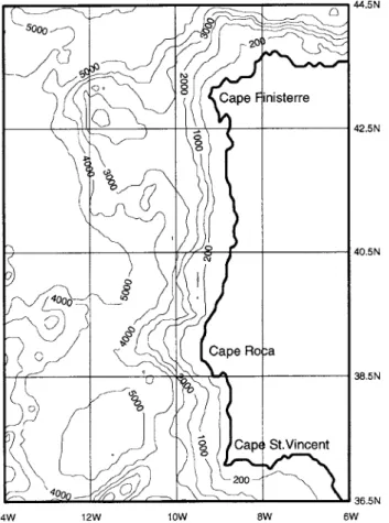
The circulation of the Atlantic Ocean off the Iberian Peninsula has a number of interesting features. The area is typical of a coastal upwelling region in the eastern bound-ary of the subtropical ocean. The winds over the region are dominated by the Azores High and in summer, when the Portuguese trade winds blow at their strongest from the north, coastal upwelling occurs. A feature of upwelling in the region is the formation of filaments of cool water extending far offshore from the coast. During autumn as the trade winds relax, the upwelling ceases and a narrow poleward surface current forms over the upper slope. The region is therefore an area of great variability on time scales ranging from seasonal, associated with the summer coastal upwelling to much shorter scales of a few days associated with the development of filament structures. The topography has an important effect on the circulation and is characterised by a narrow shelf bounded by a steep continental slope which is indented by deep narrow canyons.

Coastal features include three major capes whose position is also reflected in the bottom topography.

A European Union research project was set up to investigate various aspects of the circulation over the Iberian shelf-slope region, in particular to gain an under-standing of processes involved in the transfer of matter, momentum and energy across the shelf, shelf-break and slope. The project, called MORENA, uses a multidisi-plinary approach involving physical, chemical and biological observations, satellite imagery of the ocean surface and modelling. This work describes one approach to model-ling the region using a primitive equation ocean general circulation model. Although leading to a description of the circulation of the region this study is mainly concerned with the influence of open boundary forcing on the ability of the model to produce a realistic circulation.

The requirements of the model are manifold. The grid resolution should ideally be fine enough to adequately resolve the bottom topography and to represent correctly the mesoscale features of the circulation such as eddies, filaments and narrow slope currents. The importance of resolution has been demonstrated by a number of authors including Willebrand et al. (1994). Surface forcing by winds, heat and salt fluxes must be incorporated on time scales which adequately represent the seasonal variation of these forcing fields.

With a regional scale model such as this a major difficulty which arises is where to place the model bound-aries. The approach here is to use realistic open boundary conditions to the north, south and west of the model domain. The particular open boundary conditions em-ployed here were developed for primitive equation models by Stevens (1990) and used successfully in the UK Fine-Resolution Antarctic Model (FRAM Group, 1991). The presence of open boundaries on three sides of the model domain produces a difficult modelling problem. The at-tempts to overcome these problems are described here. The study is organized as follows. A brief description of the oceanography of the region is given in Sect. 2. The model is described in Sect. 3 with emphasis on the open boundary conditions. The model results from four

(3)

Fig. 1. Topography of the Iberian shelf-slope region. Depths in metres

experiments of increasing complexity are described in Sect. 4, with a summary and discussion in Sect. 5.

2 Oceanography of the region

A brief description is given here of the main physical oceanographic features of the region to provide a frame-work for discussing the model development and results. In this context the region under consideration is the eastern boundary of the Atlantic Ocean from the Iberian coast out beyond the shelf break to 14°W and extending from Cape Finisterre in the north to Cape St Vincent in the south, illustrated in Fig. 1. The submarine ridge associated with Cape Roca is evident as well as the complex topogra-phy with a narrow shelf and steep continental slope.

The summer season is characterised by strong norther-ly winds leading to coastal upwelling. In winter, as the Azores High relaxes southwards the winds become weaker and more generally westerly with episodes of southerly winds.

The surface circulation is generally equatorward with a southwards jet over the shelf and shelf break in summer in response to the upwelling favourable winds. A persist-ent feature observed in winter is a narrow poleward cur-rent of warm saline water over the upper slope. This current, (which is referred to later as the poleward current)

has a width of O(25 km) and extends from the surface down to O(200 m). The existence of this feature has been confirmed by satellite imagery, in situ hydrographic measurements and Lagrangian drifters, (Frouin et al., 1990; Haynes and Barton, 1990). According to Frouin et

al. (1990) only about one fifth of the observed transport of

this current can be accounted for by onshore Ekman convergence induced by southerly winds. The remainder of the transport is postulated to be due to a mechanism similar to that for the Leeuwin Current off West Australia, (McCreary et al., 1986). An oceanic baroclinic meridional pressure gradient drives an eastwards flow which induces downwelling at the coast and an associated poleward current. The current is observed only in winter as the equatorward winds in summer are strong enough to drive an equatorward current which overwhelms the poleward current.

Water masses in the area include eastern North Atlan-tic Central Water (ENACW), (Fiu´za, 1984) which occupies the main thermocline. The upper limit of the ENACW is characterised by a salinity maximum at depths around 120 m, and the lower limit by a salinity minimum at depths of about 500 m. Below the ENACW the region is influenced by Mediterranean Water (MW) which moves northwards along the slope in the form of two cores. The upper core is characterised by a temperature maximum at about 700 m and the lower core by a salinity maximum at a mean depth of 1000 m.

Satellite imagery of the sea surface has confirmed the eddy rich nature of the circulation and also provides evidence of upwelling filaments (Haynes et al., 1993). A band of cool upwelled water generally appears along the coast in late May or early June. The filaments begin to form around late July, first as bulges on the upwelling front which then grow offshore reaching their maximum extent of 200—250 km by September. The delay between the first evidence of cool upwelled water and the appear-ance of the filaments may be a form of preconditioning related to the instability process by which the filaments are generated. The filaments have widths of O(30 km) and are separated from the surrounding oceanic water by strong temperature fronts. Typically, five filaments form along the Iberian Peninsula during an upwelling season and their alongshore position appears to be related to major topographic features. They are associated with strong offshore jets (O(0.3 m s~1)) and therefore they may also play an important role in the exchange of water across the shelf break.

Another feature which is evident from satellite images in both summer and winter is a large tongue of relatively cool water extending offshore and southwards from Cape Roca.

This work is concerned with the Iberian upwelling area in the northeast Atlantic. Similar circulations patterns occur in the upwelling regions of the northeast Pacific. Models of the Oregon upwelling have recently been de-scribed by Federiuk and Allen (1995). They have carried out 60-day simulations using a sigma coordinate primitive equation two-dimensional model. They are able to predict many of the features of the Oregon upwelling, but it is clear from their work that a three-dimensional model is

(4)

required for more realistic simulations. Haidvogel et al. (1991) have used a semi-spectral primitive equation model with representative (but not realistic) topography and coastal geometry of the Californian shelf. The model is initialised as a coastal jet and filaments form near the model cape. There is no wind forcing. The results are compared with the coastal transition zone experiment. A review of modelling in shelf regions is included in the extensive review article by Huthnance (1995).

3 Model description

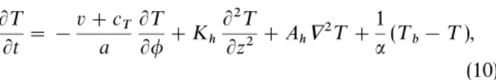
The model described here is a primitive equation level model in which the equations of motion are solved using finite differences on an Arakawa ‘B’ grid following Cox (1984). Realistic open boundary conditions are incorpo-rated and forcing is by climatological temperature, salin-ity and wind fields. The equations of motion, which have been widely quoted before are reproduced here as they form a basis for understanding the open boundary condi-tions. The full equations are

.

The variables /, j, z, u, v, w, p, o represent latitude, longitude, depth, zonal velocity, meridional velocity, verti-cal velocity, pressure and density respectively. The radius of the Earth is a, g is the acceleration due to gravity,o0 is a reference density and f"2X sin / is the Coriolis para-meter where X is the speed of angular rotation of the Earth. The variable ¹ represents any tracer including active tracers such as potential temperatureh and salinity

S or passive tracers such as tritium. Am and Ah are the

horizontal mixing coefficients for momentum and tracers.

Km and Kh are the corresponding vertical mixing

coeffi-cients.

a cos/ H 0 : ~H Fu!C (u) dz

BD

(7) where !1 a Lt L/" 0 : ~H u dz, 1 a cos/ Lt Lj" 0 : ~H v dz.

Details of the equations for the baroclinic velocities and the method of solution which involves solving separately for the tracers, baroclinic velocities and stream function are given in Cox (1984).

The open boundary conditions are due to Stevens (1990). The baroclinic velocities and tracers are calculated at the boundary using simplifications of their interior predictive equations. The baroclinic velocities are cal-culated from the following linear form of the equations of motion Lu Lt!fv"! 1 o0acos/ Lp Lj#Fu, (8) Lv Lt#fu"! 1 o0a Lp L/#Fv. (9)

This provides a reasonable approximation if the open boundaries are positioned where the non-linear terms are

(5)

Fig. 2. Model domain and topography. Depths in metres. Dotted line indicates 40.75°N zonal section

small. The equation used to calculate the tracers at a northern or southern boundary is

L¹ Lt"!v#cTa L¹ L/#Kh L2¹ Lz2#Ah+2¹# 1 a(¹b!¹), (10) where cT is the phase speed of waves propagating perpen-dicular to the boundary and is calculated using a radi-ation condition at the previous time step. The sign of the phase speed and the normal component of the advective velocity determines whether the situation is one of inflow or outflow. For the inflow situation both cT and v are set to zero. Equation (10) includes a relaxation to climatologi-cal boundary values ¹b, on a time sclimatologi-cale a. The relaxation time scalea is 360 days corresponding to the annual mean boundary climatology. For an open western boundary a similar equation to Eq. (10) is used with the meridional advective term replaced by a zonal one. This formulation for the boundary tracers is different from that used by Stevens (1990) as he used Eq. (10) without the relaxation term for outflow, and only a relaxation to climatology for inflow. Early experiments using the original Stevens (1990) form of the open boundary conditions showed that where inflow and outflow occurred at adjacent boundary points for long periods, unacceptably large lateral density gradi-ents built up causing large baroclinic velocities and viola-tion of the CFL condiviola-tion.

The barotropic streamfunction is obtained by solving the elliptic Eq. (7) and therefore requires boundary values to be specified. There is no useful simplification of Eq. (7) and therefore two other approaches to providing bound-ary stream function values are considered. One way of obtaining these values, due to Stevens (1991), and appro-priate to mid-latitudes is to use the Sverdrup balance Lt Lj"! a 2X cos /

A

L L/(qj cos /)! Lq” Lj

B

. (11) Boundary stream function values are calculated using Eq. (11) at every time step. For each zonal row of grid points, Eq. (11) is integrated westwards from the closed eastern boundary wheret"0 until the western boundary is reached. This method provides values fort along the entire north and south boundary rows and values for the western boundary are simply taken as the value oft at the western boundary.

A second approach is to use values of the boundary stream function from another basin scale model which encompasses the region of interest. The details of this new approach are given next.

The model domain is chosen as 37.5°N to 43.75°N and 13.67°W to 8.5°W. This includes the region in which the observational components of the MORENA project were conducted and places the open boundaries to the north, south and west in areas of relatively uncomplicated bot-tom topography. To the north of Cape Finisterre the coastline is modified to be aligned north-south rather than east-west in order to ensure that the eastern boundary is composed entirely of land points. The southern boundary is placed at 37.5°N rather than Cape St Vincent because large velocities associated with the Cape would make the

assumption of small advective terms in Eqs. (8) and (9) invalid. The bottom topography is taken from the DBDB5 dataset (US Naval Oceanographic Office, 1983), which is on a 1/12° grid. The horizontal resolution has been chosen as 1/12°]1/12° (approximately 9 km in the meridional direction and 7 km zonally) and is approxi-mately half the typical Rossby radius of 15—20 km. The model can therefore be considered eddy permitting. In order to fully resolve the complex topography and to make the model eddy resolving requires a finer resolution. However, the resolution chosen is sufficient to assess the performance of the open boundary conditions and to obtain a general circulation for the region. There is no reason why, with more computing resources a more lim-ited area finer resolution model could not be run to investigate the mesoscale dynamics. The number of verti-cal levels is chosen as 32 with thickness ranging from 20.3 m at the surface to 233 m at depth. This gives good resolution near the surface and a maximum depth of 5400 m that is comparable with depths over the Iberia abyssal plain. The raw DBDB5 data was first smoothed with one pass of a filter designed to eliminate identically 2Dx and 2Dy variation, then converted to model levels. Finally isolated bays were removed and the isobaths alig-ned perpendicular to the boundary for three grid points in from the open boundaries. The model domain and bottom topography are illustrated in Fig. 2. Comparison with Fig. 1 shows that the major features of the topography and coastline are reproduced. The dotted line in Fig. 2 indicates the position of zonal sections shown later.

The model uses eddy viscosity coefficients of 10~4 m2 s~1 for vertical mixing and 102 m2 s~1 for

(6)

horizontal mixing. The diffusion coefficients for tracers including temperature and salinity are 5]10~5 m2 s~1 vertically and 102 m2 s~1 horizontally.

The surface boundary condition Eq. (6) is incorporated by relaxing the tracers at level 1 to climatological data. These are taken from Levitus et al. (1994) for salinity and Levitus and Boyer (1994) for temperature. Depending on the particular experiment either annual mean or monthly mean data are used. For monthly mean forcing a linear interpolation in time is performed between the monthly datasets. The Levitus et al. (1994) and Levitus and Boyer (1994) data are compiled from observations and thus the near-surface values for the summer months include the signature of relatively cool, fresh upwelled water near the coast. In order that the relaxation scheme reflects only the heat and salt fluxes, the relaxation fields are derived from the surface tracer fields by imposing the values at the western boundary of the model as a uniform zonal field. In this way, latitudinally varying heat and salt fluxes are included but small-scale features are not. The surface salinity near the western boundary has isohalines aligned east-west and therefore a latitudinally varying salt flux is considered appropriate. The boundary relaxation fields for inflow ¹b, are annual mean data taken from Levitus (1982). The relaxation time constanta is chosen as 30 days for the surface relaxation, and 360 days for the boundary relaxation.

The surface wind stress is obtained as a linear interpo-lation between the monthly mean datasets from either Hellerman and Rosenstein (1983) or ECMWF (1993).

For the case where the boundary stream function data is specified this is taken from the Community Modelling Effort (CME) model of the North Atlantic (Willebrand

et al., 1994). The CME model has a resolution of 2/5°]

1/3°, but is also forced by Hellerman and Rosenstein (1983) winds. The four seasonal average datasets of the stream function from the CME model were interpolated onto the boundary of the MORENA model, and a linear interpolation in time between these datasets provided the required boundary stream function.

For all runs the model was initialised to a state of rest and with climatological values for the temperature and salinity from Levitus (1982). This data, which is on a 1°]1° grid is first extrapolated horizontally to cover the model domain including land points, then interpolated horizontally and vertically onto the model grid points. Early runs were initialised to the annual mean salinity from Levitus et al. (1994) and temperature from Levitus and Boyer (1994). The combination of the extrapolated temperature and salinity, and the steep topography result-ed in large bottom pressure torques over the continental slope. This caused slow convergence of the stream func-tion, large barotropic velocities and the model quickly going unstable. The earlier atlas, Levitus (1982), is much smoother and starting with this annual mean data caused no instability problems. Time series of temperature and salinity data for runs with monthly mean surface and annual boundary forcing show an adjustment away from the Levitus (1982) initial data which is completed during the first year of the model run. By year 3 the model has settled into a repeating annual cycle.

4 Model results

The development of the model is presented here as results from a series of experiments. In chronological order the model increases in complexity and serves to illustrate the importance of including particular features. The results focus mainly on the winter circulation as this includes the near surface poleward current. The upwelling situ-ation in summer has, by contrast, been modelled many times. The final model provides a realistic description of the general circulation of the region. Four experiments are selected for presentation here and are variations on the basic model.

A: Sverdrup boundary stream function Annual mean surface relaxation of tracers Annual mean boundary relaxation of tracers Hellerman and Rosenstein winds

B: Specified boundary stream function Annual mean surface relaxation of tracers Annual mean boundary relaxation of tracers Hellerman and Rosenstein winds

C: Specified boundary stream function Monthly mean surface relaxation of tracers Annual mean boundary relaxation of tracers Hellerman and Rosenstein winds

D: Specified boundary stream function Monthly mean surface relaxation of tracers Annual mean boundary relaxation of tracers ECMWF winds

Results are presented as horizontal sections of velocity at level 2 (32 m), temperature at level 1 (10.3 m); and zonal or meridional sections of cross-track velocity, temperature and salinity. The horizontal sections of velocity are shown at level 2 as this is representative of the near surface circulation without including Ekman effects. Temper-atures are shown at level 1 as this allows comparison with satellite images of sea surface temperature. The zonal and meridional sections are presented for depths from the surface to 1287 m, as this range includes the more interest-ing features of the circulation. The zonal sections are shown at 40.75°N as this section includes generally uni-form topography. The model is started from 1 January year 1 and the sections are all shown at either 1 March year 3, referred to as winter or 31 August year 3, referred to as summer.

4.1 Case A

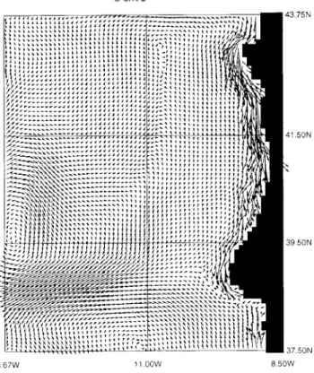
This first version of the model uses the Sverdrup balance to obtain boundary stream function data and the relaxa-tion at the surface and open boundaries is to annual mean tracer fields. Winds are taken from Hellerman and Rosen-stein (1983), which are more morthwesterly in the north of the region than is presently observed. The winter velocity field at level 2 (32 m) is shown in Fig. 3. The circulation is generally weak except over the shelf in the north of the region where the equatorward flow reaches 10 cm s~1 in response to the northwesterly winds. In the south there is a broad poleward flow extending from the coast to 11°W which reaches Cape Roca before turning offshore. The

(7)

Fig. 3. Winter velocity field at level 2 (32 m) for case A with Sver-drup boundary stream function, annual mean surface and boundary relaxation of tracers, and driven by Hellerman and Rosenstein winds

Fig. 4. a Winter velocity field at level 2 (32 m) and b winter temper-ature at level 1 (10.3 m) for case B with boundary stream function from the CME North Atlantic model, annual mean surface and boundary relaxation of tracers, and driven by Hellerman and Rosen-stein winds

summer circulation is similarly weak with the exception of a stronger equatorward flow over the shelf.

Although the method of deriving boundary stream function data using the Sverdrup balance has performed well in the UK Fine-Resolution Antarctic Model (FRAM Group, 1991), for this shelf-slope model it clearly produces unrealistic results with none of the expected features de-scribed already. In this model of the Iberian part of the North Atlantic, the flow is not dominated by Sverdrup dynamics but by the eastern boundary currents. The pres-ence of three open boundaries also makes the application of the Sverdrup type boundary condition difficult.

4.2 Case B

The results of case A demonstrate that an alternative method of specifying the boundary stream function is needed. As described in Sect. 3 stream function data is taken from the CME North Atlantic model and imposed on these model boundaries. In other respects this experi-ment remains the same as case A with relaxation to annual mean tracers and wind forcing from Hellerman and Rosenstein (1983).

The winter circulation at level 2 (32 m) is shown in Fig. 4a. Comparison with Fig. 3 shows that a much more realistic circulation is obtained in this case as a result of simply changing the boundary stream function. The flow is generally equatorward over much of the region with velocities up to 7 cm s~1. There is still an equatorward

flow close to the coast in the north due to the northwester-ly winds and also a narrow poleward flow over the upper slope which reaches from the open southern boundary to 42°N. The level 1 temperature field shown in Fig. 4b

(8)

shows the effect of this poleward current advecting warm water northwards close to the coast. The summer results are not illustrated as they are similar to the case C results described fully later. However, the near surface circulation is also equatorward with a southwards jet over the shelf and the associated cool upwelled water. The poleward current over the upper slope is absent in summer. This case would appear to give a good description of the circulation, although the strength of the poleward current in winter decreases year by year as the model integration is continued. The mechanism for the poleward flow pro-posed by Frouin et al. (1990), described in Sect. 2, relies on a baroclinic oceanic meridional pressure gradient. A weakening of this pressure gradient over time will result in a corresponding weakening of the poleward flow. The near surface flow is generally equatorward through-out the year and results in cool water being advected southwards from the open northern boundary. The effect is a gradual cooling of the whole model domain and a weakening of the meridional pressure gradient and the poleward current in winter. The suface relaxation to annual mean data does not provide seasonal warming of the near surface layers to maintain the meridional pres-sure gradient. This poor performance of the model is solely due to using annual mean data for the surface relaxation fields.

4.3 Case C

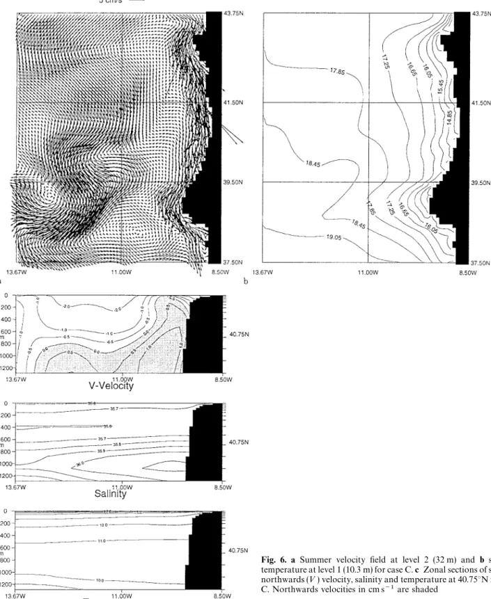
A solution to the problem of cooling of the model in case B is to use monthly mean forcing from Levitus et al. (1994) and Levitus and Boyer (1994) at the surface. The bound-ary stream function data is again from the CME model and forcing is by Hellerman and Rosenstein winds. The results for the winter velocity and temperature fields are shown in Fig. 5a, b; a zonal section along 40.75°N is shown in Fig. 5c and a meridional section along 11°W in Fig. 5d. The velocity field is similar to that for case B with a general equatorward flow except over the upper slope where the narrow poleward flow is evident. The pattern of level 1 temperatures are similar to case B although the actual temperatures over the whole region are lower in Fig. 5b than in Fig. 4b due to the seasonal forcing. The effect of the poleward current advecting warm water northwards is also clear. The width of the current is approximately 30 km extending to a depth of 200 m. These values are in accord with the observations of Frouin et al. (1990). The effect of the current is also evident in the salinity field. Figure 5c shows the northwards ad-vection of Mediterranean water with salinity '36.1 at about 1000 m near the coast, the southwards flow of the low salinity ENACW above this and the well-mixed sur-face layer with a temperature of 14 °C down to 75 m. The water masses of the region are illustrated well in Fig. 5d with two cores of Mediterranean Water, the temperature maximum at 700 m and the salinity maximum at 1000 m both being brought northwards into the model domain through the open southern boundary. Also evident is the salinity minimum of the ENACW with weak stratification between 100 m and 500 m.

The corresponding pictures for the summer situation are shown in Fig. 6a—c. In Fig. 6a the equatorward flow over the whole region is stronger in response to the stron-ger trade winds particularly over the continental shelf. No poleward flow over the upper slope is evident. The level 1 temperatures in Fig. 6b clearly show the upwelling near the coast with higher temperatures over the remainder of the region. The tongue of cool water off Cape Roca often seen in satellite images is evident here. The zonal section at 40.75°N in Fig. 6c confirms the absence of the near surface poleward flow over the upper slope and shows a poleward countercurrent below the equatorward up-welling jet. The zonal section of temperature also shows the near surface summer thermocline. A meridional sec-tion for the summer situasec-tion is not shown as it is similar to the winter case. A final illustration of the monthly nature of the forcing in this case is given in Fig. 7 with a 3 year time series of temperatures from levels 1 to 6 at 40°N, 12°W. The seasonal variation in the surface forcing is clearly seen, the effect penetrating down to level 4 (86 m). In each year, the winter cooling results in levels 1 and 2 becoming isothermal around early January with level 3 convectively mixing around early March. The effect of summer heating quickly increases the temperature of level 1 from the end of April with levels 2 and 3 responding more slowly.

For runs carried on longer than 3 years the monthly forcing maintains the near surface meridional temperature gradient whereas the annual forcing in case B cannot. The general cooling of the model in case B and the loss of the meridional pressure gradient results in a gradual weaken-ing of the poleward current over a period of several years confirming the generation mechanism described in Sect. 2.

4.4 Case D

A comparison of the winds from Hellerman and Rosen-stein (1983) with other datasets suggest that they have too great a northerly component over the north of the region in winter. The winds over the northeast corner of the model domain should be southwesterly rather than the northwesterlies in Hellerman and Rosenstein (1983). The effect of the northwesterlies is to generate a southwards flow near the coast which prevents the near surface part of the poleward current penetrating further north than 42.5°N, whereas observations by Frouin et al. (1990) indi-cate that the current extends the full length of the Iberian Peninsular.

An alternative wind dataset is the ECMWF winds (ECMWF, 1993) averaged over the years 1986 to 1988. The relatively short averaging period results in a wind field which is less climatological but which has a south-westerly component in winter over the north of the model domain. Case D is the same as case C in all respects except that it is driven by ECMWF winds rather than Hellerman and Rosenstein winds.

The winter circulation for case D is shown in Fig. 8. The poleward current can be traced along the whole coast and out through the northern boundary of the model, and so extends much further north than case C. With the

(9)

Fig. 5. a Winter velocity field at level 2 (32 m) and b winter temper-ature at level 1 (10.3 m) for case C. Same conditions as for Fig. 4 except for monthly mean surface relaxation of tracers. c Zonal sections of winter northwards (» ) velocity, salinity and temperature

at 40.75°N, and d meridional sections of eastwards (º ) velocity, salinity and temperature at 11°W for case C. Northwards and eastwards velocities in cm s~1 are shaded

(10)

Fig. 6. a Summer velocity field at level 2 (32 m) and b summer temperature at level 1 (10.3 m) for case C. c Zonal sections of summer northwards (» ) velocity, salinity and temperature at 40.75°N for case C. Northwards velocities in cm s~1 are shaded

influence of the southwesterly winds the flow over the shelf is also northerly in winter, which contrasts with the south-wards flow over the shelf in case C in response to the northwesterly winds. The southerly flow over the shelf around 43.75°N is simply a barotropic effect due to the

imposed boundary stream function. The flow in Fig. 8 generally provides a good comparison with observations although the magnitude of the poleward current is not as strong in the north as the observations of Frouin et al. (1990).

(11)

Fig. 7. Time series of temperatures for levels 1 to 6 at 40°N, 12°W for case C. ¸evel 1 (10.3 m), level 2 (32 m), level 3 (57 m), level 4 (86 m),

level 5 (120 m) and level 6 (162 m) Fig. 8. Winter velocity field at level 2 (32 m) for case D with ECMWF winds. Compare with Fig. 5a for case C with Hellerman and Rosenstein winds

5 Summary and discussion

The use of the described open boundary conditions for a primitive equation ocean model has allowed a fine-resolution regional model with three open boundaries to be run at a relatively low computational cost. The results obtained for the circulation and temperature fields are realistic and reproduce many of the features seen in the observations. The use of a rigid lid model requires bound-ary stream function values to be specified and the results indicate that this part of the open boundary condition is critical in obtaining realistic results.

The model generates the poleward current observed by Frouin et al. (1990), in winter outside the upwelling sea-son. The strength of this poleward current weakens over time if annual mean surface forcing is used. The use of seasonal surface forcing can maintain a meridional pres-sure gradient thus supporting the generation mechanism proposed by Frouin et al. (1990). The use of ECMWF wind forcing, which appears closer to the perceived winter winds than Hellerman and Rosenstein, allows the pole-ward current to extend to the surface along the entire eastern model boundary also suggesting that the current is partly wind driven. However, the poleward current is not as strong as observations suggest. It is thought that the weaker current is due to poor input data at the northern boundary, and further numerical experiments are being carried out to try and improve this result.

During the upwelling season, the model has upwelling along the coast associated with an equatorward jet over the shelf and a poleward countercurrent close to the slope. The surface temperature field has cool upwelled water

close to the coast but does not exhibit any significant filament structure, although there are many eddies. A strong temperature front is necessary for the formation of filaments, whereas the horizontal mixing in level models tends to inhibit the formation of strong fronts. An experi-ment with the horizontal diffusion of heat and salt halved to 50 m2 s~1 has been carried out. In this case the temper-ature field includes an upwelling front that is non-uniform along the coast with the beginnings of filament formation. To model the generation of filaments satisfactorily in a primitive equation level model requires a much finer resolution and reduction of the mixing coefficients. Runs with a simple channel model indicates that a resolution of 2.3 km and values Am"10 m2 s~1, Ah"1 m2s~1 results in filament formation.

The meridional and zonal sections of temperature and salinity described in Sect. 4 reveal the water mass structure of the region. The Mediterranean water is allowed to enter the model at the southern boundary and can be followed northwards through the temperature maximum at 700 m and the salinity maximum at 1000 m. A band of weakly stratified, low salinity eastern North Atlantic Central Water enters through the open northern boundary. The inflow of these water masses and the ability of the model to respond to seasonal forcing indicate that the open boundary conditions are performing well. Indeed, anima-tions of the temperature field and stream function show that no false reflection of outgoing waves occurs at the open boundaries. A much more detailed analysis of the model output will be carried out as the results of the

(12)

observational component of the MORENA project become available.

The results presented here show that a fine-resolution model with three open boundaries and seasonal forcing can reproduce the main features of the circulation in an area of complex topography and hydrography.

Acknowledgements. The MORENA project is financed by the Euro-pean Union MAST II programme under contract number MAS2-CT93-0065. Thanks are due to David Stevens and Martin Wadley for discussions concerning the open boundary conditions, and to an anonymous referee for a thorough and constructive review. We are indebted to Rene Redler (Institut fu¨r Meereskunde, Kiel) who pro-vided the CME stream function data.

Topical Editor D. Webb thanks J. M. Huthnance and B. Hackett for their help in evaluating this paper.

References

Cox, M. D., A primitive equation 3-dimensional model of the ocean, Geophys. Fluid Dyn. ¸ab. Ocean Group ¹ech. Rep., 1, 143 pp., 1984.

ECMWF, The description of the ECMWF/WCRP level III-A atmo-spheric data archive, Technical Arttachment, ECMWF, Shinfield Park, Reading, UK, 1993.

Federiuk, J., and J. S. Allen, Upwelling circulation on the Oregon Continental shelf, Part II. Simulations and comparisons with observations. J. Phys. Occeanogr., 25, 1867—1989, 1995 Fiu´za, A. F. G., Hidrologia e Dinaˆmica das A¨guas Costeiras de

Portugal, Ph.D. Dissertation, Universidade de Lisboa, Portugal, 1984.

FRAM Group, Initial results from a fine resolution model of the Southern Ocean, EOS, ¹rans. Am. Geophys. ºnion, 72, 169, 174—175, 1991.

Frouin, R., A. F. G. Fiu´za, I. Ambar, and T. J. Boyd, Observations of a poleward surface current off the coasts of Spain and Portugal during winter, J. Geophys. Res., 95, 679—691, 1990.

Haidvogel, D. B., A. Beckmann, and K. S. Hedstro¨m, Dynamical simulations of filament formation and evolution in the coastal transition zone, J. Geophys. Res., 96, 15017—15040, 1991. Haynes, R., and E. D. Barton, A poleward flow along the Atlantic

coast of the Iberian Peninsular, J. Geophys. Res., 95, 11425—11441, 1990.

Haynes, R., E. D. Barton, and I. Pilling, Development, persistence and variability of upwelling filaments off the Atlantic Coast of the Iberian Peninsular, J. Geophys. Res., 98, 22681—22692, 1993. Hellerman, S., and M. Rosenstein, Normal monthly wind stress over the world ocean with error estimates, J. Phys. Oceanogr., 13, 1093—1104, 1983.

Huthnance, J. M., Circulation, exchange and water masses at the ocean margin: the role of physical processes at the shelf edge, Prog. Oceanogr., 35, 353—431, 1995.

Levitus, S., Climatological atlas of the world ocean, NOAA Prof. Pap. 13, 173 pp., US Government Print Office, Washington, D.C., 1982.

Levitus, S., and T. Boyer, ¼orld ocean atlas 1994, »ol. 4: ¹emper-ature, NOAA Atlas NESDIS 4, NOAA Washihgton D.C., 1994. Levitus, S., R. Burgett, and T. Boyer, ¼orld ocean atlas 1994, Vol. 3: Salinity, NOAA Atlas NESDIS 3, NOAA Washington D.C., 1994.

McCreary, J. P., S. R. Shetye, and P. K. Kundu, Thermohaline forcing of eastern boundary currents: with application to the circulation off the west coast of Australia, J. Mar. Res., 44, 71—92, 1986.

Stevens, D. P., On open boundary conditions for three-dimensional primitive equation ocean circulation models, Geophys. Astro-phys. Fluid Dyn., 51, 103—133, 1990.

Stevens, D. P., The open boundary condition in the United King-dom fine-resolution antarctic model, J. Phys. Oceanogr., 21, 1494—1499, 1991.

US Naval Oceanographic Office, DBDB5 (Digital Bathymetric Data Base — 5-minute grid), U.S.N.O.O., Bay St. Louis, Mississippi, US, 1983.

Willebrand, J., A. Beckmann, C. W. Bo¨ning, and C. Koberle, Effects of increased horizontal resolution in a simulation of the North Atlantic ocean, J. Phys. Oceanogr., 24, 326—344, 1994.