Nonparametric catchment clustering using the data depth function.

1 Publisher: Taylor & Francis & IAHS

Journal: Hydrological Sciences Journal DOI: 10.1080/02626667.2016.1168927

Non-parametric catchment clustering using the data depth function

1

National Institute of Water and Atmospheric Research, Christchurch, New Zealand 2

Department of Geography, San Diego State University, San Diego, USA 3

Institute for Modelling Hydraulic and Environmental Systems, University of Stuttgart, Stuttgart, Germany 4

Institut National de la Recherche Scientifique, Centre Eau Terre Environnement, Québec-city, Canada

Abstract

The clustering of catchments has been important for prediction in ungauged basins, model parameterization and watershed development and management. The aim of this study is to explore a new measure of similarity among catchments, using a data depth function and comparing it with catchment clustering indices based on flow and physical characteristics. A

cluster analysis was performed for each similarity measure using the affinity propagation

clustering algorithm. We evaluated the similarity measure based on depth-depth plots (DD-plots) as a basis for transferring parameter sets of a hydrological model between catchments. A case study was developed with 21 catchments in a diverse New Zealand region. Results show that clustering based on the depth-depth measure is dissimilar to clustering on catchment characteristics, flow, or flow indices. A hydrological model was calibrated for 21 catchments and the transferability of model parameters among similar catchments was tested within and between clusters defined by each clustering method. The mean model performance for parameters transferred within group always outperformed those from outside the group. The DD-plot based method was found to produce the best in-group performance and second-highest difference between in-group and out-group performance.

2

Keywords: DD-plot, catchment similarity, data depth, affinity propagation clustering

1 Introduction

The organization and clustering of catchments has been important for prediction in ungauged basins, model parameterization and watershed development and management. If we could transfer parameters from one catchment to other similar catchments, this would avoid the need to calibrate the model everywhere, saving time and computer resources and enable model use in ungauged catchments. However, even if precipitation, vegetation or other catchment characteristics are similar, the hydrological response of catchments can be very different (Beven 2004). The hydrological response depends on various known and unknown physical and climatic characteristics of the catchment. Hence, defining the similarity between two catchments is a complex multivariate problem. In higher dimension data, many attributes may be irrelevant; hence grouping of similar catchments based on many signatures can be a very difficult task. Even today there is no robust definition for similarity between two catchments, due to our limited knowledge about very complex nonlinear hydrological phenomenon (Wagener et al. 2007, Ali et al. 2012).

Using a similarity measure, we can primarily cluster catchments. This is important for many reasons, for example, for prediction in ungauged catchments, model parameterization and regulation or management of watershed development. Catchment clustering into groups based on hydrological response or catchment characteristics is the first step toward regionalization of flow characteristics. In addition, policies for watershed development in one catchment might be transferable to other catchments in that group. McDonnell and Woods (2004) defined the basic needs of any catchment clustering scheme. They advocated that “a catchment hydrology clustering system would provide an important organising principle, complementing the concept of the hydrological cycle and principle of mass conservation”. Clustering can also help in choosing appropriate models for poorly understood hydrological

3

systems. There continue to be many studies (Ali et al. 2012, Cheng et al. 2012, He et al. 2011, Ley et al. 2011, Post and Jakeman, 1999, Samaniego et al. 2010, Wagener et al. 2007, Sawicz et al. (2011)) on catchment clustering, but no silver bullet exists to specify relevant measures of catchment similarity. Catchments can be clustered based on their characteristics, fluxes or signatures.

1.1 Methods for catchments clustering

Despite many studies in the field of catchment clustering, hydrology does not yet possess a generally agreed upon catchment clustering system (Wagener et al. 2007). Recent examples include a catchment clustering scheme based on a local variance reduction method (He et al. 2011). Ley et al. (2011) used a self-organizing map (SOM) to define catchment similarity based on catchment response behaviour and characteristics. They found that similarity based on flow characteristics overlapped 67 % with similarity defined by catchment characteristics. In another study by Thod (2013) where a catchment clustering was conducted based on characterisation of streamflow and precipitation series using SOM. The study found that inclusion of information on the properties of the fine time-scale streamflow and precipitation time series may be a promising way for better representation of the hydrologic and climatic character of a catchment. Samaniego et al. (2010) proposed a dissimilarity measure that is estimated from pairwise empirical copula densities of runoff and applied for streamflow prediction in ungauged catchments. Sawicz et al. (2011), conducted an empirical analysis of hydrologic similarity based on catchment function in the eastern USA for catchment clustering. They defined six signatures from precipitation-temperature-streamflow and used a Bayesian clustering scheme to separate the catchments into nine homogeneous clusters. They found that most of the clusters exhibited some degree of connectivity suggesting that spatial proximity is a good indicator of similarity. In a series of three papers about comparative assessment of prediction in ungauged basins, in part 1 and 2, Parajka et al. (2013) and Salinas

4

et al. (2013) assessed the regionalisation performance of hydrographs and hydrological extremes on the basis of a comprehensive literature review of thousands of case studies around the world. In a continuation, Viglione et al. (2013) assessed prediction performance of a range of runoff signatures for a consistent and rich dataset by rationalised rainfall-runoff model and Top-kriging methods in Austria. Their comparative assessment showed that, in Austria, the predictive performance increases with catchment area for both methods and for most signatures, it tends to increase with elevation for the regionalised rainfall–runoff model, while the dependence on climate characteristics is weaker. More details about prediction in ungauged basin can be found in the review paper of Hrachowitz et al. (2013).

1.2 Catchment clustering for regionalisation

The aim of catchment clustering is to define hydrologically homogeneous groups so that information can be transferred between catchments of the group and the parameters of hydrological models from one catchment can be transferred to other catchments.

1.2.1 Examples of methods

The example to define homogeneous hydrological groups and transfer the model parameters within the group can be seen in many studies. e.g. He et al. (2011) presented a catchment clustering scheme based on a local variance reduction method with model performance as a

similarity measure. In a study covering 90 natural watersheds across the Province of Ontario,

Canada, Razavi and Coulibaly (2013) found that nonlinear clustering methods like Self Organizing Maps (SOMs), standard Non-Linear Principal Component Analysis (NLPCA) and Compact Non-Linear Principal Component Analysis (Compact-NLPCA) can be robust tools for the clustering of ungauged catchments prior to regionalization. Merz and Blöschl (2004) examined eight regionalization methodologies in 308 catchments in Austria. They found that the best regionalization methods are those that rely on spatial proximity: either using the average parameters of immediate upstream and downstream neighbours or

5

regionalization by kriging. In a similar study, Parajka et al. (2005) found that the kriging and similarity approaches where parameters from immediate neighbours are transferred to catchment of interest performed best. A comprehensive overview of regionalization methodologies and different approaches can be found in Blöschl (2005), Vogel (2006) and Wagener et al. (2004).

1.3 Contribution of this paper

In this paper, we propose a new non-parametric similarity measure for catchment clustering, based on the concept of data depth function. The data depth function is a robust tool to rank multivariate datasets (Dutta and Ghosh 2012). We use Depth-Depth plots (DD-plots; described in Section 2.2) to define catchment similarity based on catchment response behaviour. The major advantage of a DD-plot based catchment similarity measure is that it uses the full time series instead of statistics of the series, where the latter loses information through the averaging effect. Our proposed method uses the whole dynamics of the series. For comparison, we also identify hydrologically similar catchments based on physical catchment characteristics and flow indices. We then use each similarity measure to identify

groups of similar catchments using the recently developed clustering algorithm called affinity

propagation (AP) (Frey and Dueck 2007). The advantage of AP clustering is that in addition to partition of the objects of a dataset into groups of similar objects, it also identifies a single object that is most representative of each group. In hydrological model parameter transfer applications, this property is particularly useful as we can calibrate the model for this representative catchment, and then transfer the model parameters to other catchments in that group. We compare the catchment grouping as well as the success of parameter transfer within group, using the data-depth similarity measure vs. similarity measures based on physical catchment characteristics or flow indices.

6

Twenty-one catchments from the Bay of Plenty region in the North Island of New Zealand were used in this study. The reason for choosing this region is that the catchments have a wide range of different topographic properties, response behaviour and geology; in particular part of the region has highly damped flow behaviour due to pumice-rich volcanic soils. This paper is organized as follows: After the introduction, the methodology is presented in Section 2. The case study and model calibration are introduced in Section 3. The results are discussed in Section 4. In the final section conclusions are drawn.

2 Methodology

In this section, we first define the data depth function and then show how it can be used to

define catchment similarity via a DD-plot. We then describe the affinity propagation (AP)

clustering method for catchment clustering.

2.1 Data Depth Function

Data depth is a quantitative measure expressing how central (or deep) a point is with respect to a dataset or a distribution. This gives us a central outward ordering of multivariate data points and gives rise to simple new ways to quantify the many complex multivariate features of the underlying multivariate distribution (Li et al. 2012, Liu et al. 1999). A depth function was first introduced by (Tukey 1975) to identify the centre (a generalized median) of a multivariate dataset. Several generalizations of this concept have been defined (Barnett 1976, Liu 1976, Liu et al. 2006, Rousseeuw and Struyf 1998, Zuo and Serfling 2000). Data depth functions have been applied in several fields of non-parametric multivariate analysis (Andrew et al. 2000, Hamurkaroglu et al. 2006, Liu, 1995, Liu and Singh 1993, Messaoud et al. 2004, Serfling 2002, Stoumbos et al. 2001). Application of the data depth function is relatively new in the field of water resources. It has been used in the field of regional flood frequency analysis (Chebana and Ouarda 2008, Wazneh et al. 2013a, Wazneh et al. 2013b), depth-based

7

multivariate descriptive statistics in hydrology (Chebana and Ouarda 2011b), regionalization of hydrological model parameters (Bardossy and Singh 2011) and robust estimation of hydrological model parameters (Bárdossy and Singh 2008), defining predictive uncertainty of a model (Singh et al. 2013), and in selection of critical events for model calibration (Singh and Bárdossy 2012). For more detailed information about the data depth function and its uses in field of water resources, please refer to Chebana and Ouarda (2011a), Chebana and Ouarda (2011c), Guerrero et al. (2013), Krauße and Cullmann (2009) and Singh and Bárdossy (2012).

Several types of data depth functions have been developed, e.g. half-space, L1 and Mahalanobis depth functions. The half-space data depth function was used in this study because it is a non-parametric, satisfies all the properties of the data depth function and it is robust in calculation.

Formally, the half-space depth of a point p with respect to the finite set X in the d dimensional space is defined as the minimum number of points of the set X lying on one side of a hyperplane through the point p. The minimum is calculated over all possible hyperplanes. Formally, the half-space depth of the point p with respect to set X is:

(1)

Here is the scalar product of the d dimensional vectors, and nh is an arbitrary unit

vector in the d dimensional space representing the normal vector of a selected hyperplane. If the point p is outside the convex hull of X then its depth is 0. The convex hull of a set of points S is the smallest convex set (e.g. convex polygon in 2D) which encloses S. An example of a convex hull is given in Figure 1. Points on and near the boundary have low depth while points deep inside have high depth. One advantage of this depth function is that it is invariant to affine transformations of the space. This means that the different ranges of the

(

)

8

variables have no influence on the calculated depth. In this study, we normalised the data depth between 0 and 1 by dividing the depth with half the number of total points in the convex hull.

Discharge, Antecedent Precipitation Index (API) or discharge derived indices could be used to define catchment similarity: all of these help to define the range of dynamic behaviour of a catchment. For simplicity, denote the selected series (discharge or indices) as X (t). Considering all sets of d consecutive time steps leads to a d-dimensional set which is defined by the following equation

𝑋𝑑(𝑡) = {(𝑋(𝑡 − 𝑑 + 1), 𝑋(𝑡 − 𝑑 + 2), … … . 𝑋(𝑡)) 𝑡 = 𝑑 … … . . 𝑇 (2)

where T is the total number of observation time steps available. For our case, data in hourly resolution were available. After testing different values of d, we selected d=4 hrs to reflect the dynamics and memory of the catchment. The value of d can be selected depending on the catchment (sensitive to catchment area, shape and flashiness) and it can only be found on trial based method. Based on the authors experience in different catchments, d=4 (up to 4 time step) is a typical recommendation. The following section describes how the data depth function can be used to define the catchment similarity based on catchment response behaviour.

2.2 DD-plots and its application for catchment clustering using catchment response behaviours

Many useful tools in nonparametric multivariate data analysis have been developed based on the concept of the data depth function (Li et al. 2012). Figure 2 shows how the data depth function and the convex hull can be used for defining similarity between catchments. If the convex hulls of two catchments characteristics are similar, it suggests that they have a similar

9

range of dynamic behaviour. This does not take into account the range of the variable, so it is only appropriate for normalised flow indices.

To visualise the similarity of the datasets and their convex hulls in high-dimensional space (4D in our case), we use the depth-depth-plot (Liu et al. 1999). The DD-plot is a simple graphical tool for comparing two given multivariate samples or distributions. A

d-dimensional dataset D± (Eq. 2) corresponding to catchment ± is taken, and the depth of each

element of D± is calculated with respect to D± and also to the convex hull of dataset D²

from catchment ² . The data depth of D² with respect to D± is also calculated. The DD-plot is

then created by plotting, for each data point, the depth with respect to D± against the depth

with respect toD² .

Let x be any point in the d-dimensional space. The depth of the point is calculated with

respect to the set D± and D² . This pair of depths is then plotted in a simple two dimensional

graph.

𝐷𝛼(𝑥) , 𝐷𝛽(𝑥) (3)

The calculations are restricted to x axis which are in either D± or D². If the two set are very

different than a point which is deep in one set is not deep in the other. Thus DD-plot is expressing to what extent D sets overlaps.

Formally, let ± and ² be two distributions on Rd and D (.) the depth function defined in Eq. 1.

Then the Depth-Depth plot for two distributions can be defined as

𝐷𝐷(𝛼, 𝛽) = {𝐷𝛼(𝑥) 𝑓𝑜𝑟 𝑎𝑙𝑙 𝑥 ∈ 𝛼 }𝑈 �𝐷𝛽(𝑥) 𝑓𝑜𝑟 𝑎𝑙𝑙 𝑥 ∈ 𝛽� (4)

A DD-plot is a simple graph on the plane regardless of how high the dimension of the data is (Li et al. 2012, Liu et al. 1999). Differences in location, scale, skewness or kurtosis between the two distributions will give different patterns of the DD-plots (Liu et al. 1999). Our clustering approach based on DD-plots is nonparametric as we do not fit any distribution to the data series. If the two given sets are identical, then the DD-plot is a segment of the 1:1

10

line, whereas deviations from this diagonal line indicate differences between the two sets. Hence, if the DD-plot of two catchments is close to the diagonal line, we assume the catchments have similar response behaviour. A Q (t) vs Q (t-1) (d=2) plots for two sample catchments ± and ² is shown in Figure 3(a), while the corresponding Q (t), Q (t-1) and Q (t-2) (d=3) plots for the same catchments are shown in Figure 3(b). A DD-plot where d=4 is given in Figure 3(c). Figure 3(a) and Figure 3(b) summarise the flow dynamics of the catchment in 2 and 3 dimensions where we can see that catchments ± and ² have quite similar behaviour. In Figure 3(c), the DD-plot summarises the 4 dimensional relationship between flow dynamics of catchment ± and ² . To summarise the flow dynamics of catchments, most of the time we need to visualise higher dimensions. A DD-plot can be used for plotting any data dimension in the two dimensional plane. In this study, we made the DD-plot using 4 dimensional flow data.

To make an objective clustering using DD-plot, we plotted DD-plots pair wise for all possible combinations of catchments. We chose to calculate the area of the convex hull of the DD-plot as an indicator of similarity, i.e. a smaller convex hull implies that the points are closer to the diagonal and thus the catchments are more similar. Based on this indicator, we can rank pairs of catchments from most similar to least similar. To make a systematic clustering we then used the area of the convex hull of DD-plots as the similarity matrix for a clustering algorithm. DD-plot based clustering has advantages over other clustering based on flow indices, as it can use high dimensional series of flow values and hence better represent the dynamics across multiple time steps.

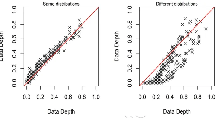
To illustrate the method we took a sample from two bivariate distributions: bivariate normal and bivariate Cauchy. We then made two DD-plots: The first using two random samples of 500 points from the same distribution (bivariate normal) and the second using random samples from two different distributions (bivariate normal and bivariate Cauchy)(Figure 4). It

11

is clear from the figure that the divergence from the diagonal line is greater for the second DD-plot. To quantify this we calculate the area of the convex hull of the points. The area of convex hull from same distribution (Figure 4(a)) is 0.043 whereas the area of the convex hull from two different distributions (Figure 4(b)) is 0.082 indicating greater dissimilarity. The same concept applies for two hydrologically similar or dissimilar catchments. The area of convex hulls from DD-plots used as a similarity measure with a clustering algorithm is described in the next section.

2.3 Catchment grouping using clustering

2.3.1 Catchment clustering

Clustering is the process of classifying objects into different groups based on their similarity. Many clustering methods are agglomerative, i.e. they start by defining small groups. Then they proceed based on a fusion technique, by combining objects with objects or with groups, or groups with groups. The technique can be displayed by a dendogram where the vertical axis shows the level of fusion. There are many agglomerative clustering methods available.

In this study we used AP clustering (Frey and Dueck 2007). An advantage of AP clustering is

that it both partitions the objects of a dataset into groups of similar objects, and identifies a single object (the “exemplar”) that is most representative for each group. Exemplar-based AP clustering provides an additional advantage for finding automatically the right number of clusters (Bodenhofer et al. 2012). In hydrological model parameter transfer, the exemplar can play an important role. We can calibrate the model for the most representative catchment of the group (the exemplar), and then transfer the parameters to other members of the group.

AP clustering does not need the user to define the number of clusters prior to the clustering.

The designers describe the method as follows: “Each object in a dataset is considered as a

node in a network; real-value messages are recursively transmitted along the edges of the network until a good set of exemplars gradually emerges. At each iteration, the magnitude of

12

each message reflects the current affinity that one object has for choosing another object as its exemplar, hence the term affinity propagation” (Ali et al. 2012, Frey and Dueck 2007).

AP simultaneously considers all the data points as possible exemplars, exchanging real-values message between them until a high-quality set of exemplars and cross ponding cluster emerged. AP finds clusters on the basis of maximising the total similarities between data points and their exemplar (Dueck 2009). The R package “apcluster” (Bodenhofer et al. 2012) was used in this study. The square similarity matrices of mutual pairwise similarities of data vectors were computed using negative square distance, i.e. given distance d, the resulting

similarity is computed as S = -dr. we used r=2 to obtain the negative square distance as

described in (Frey and Dueck 2007). A valid distance measure should be symmetrical and obtain its minimum value, usually zero, in case of exact similarity. They used Euclidean distance as the distance between two data samples.

In this study we classified the catchments based on the following variables: (1) DD-plots based on discharge, (2) flow duration curve indices, (3) flow indices, (4) and catchment properties. To classify based on flow duration curve, we fit a two parameter (shape and rate)

Gamma distribution (using Equation 5, where ± and 𝛿 are shape and rate parameters) as used

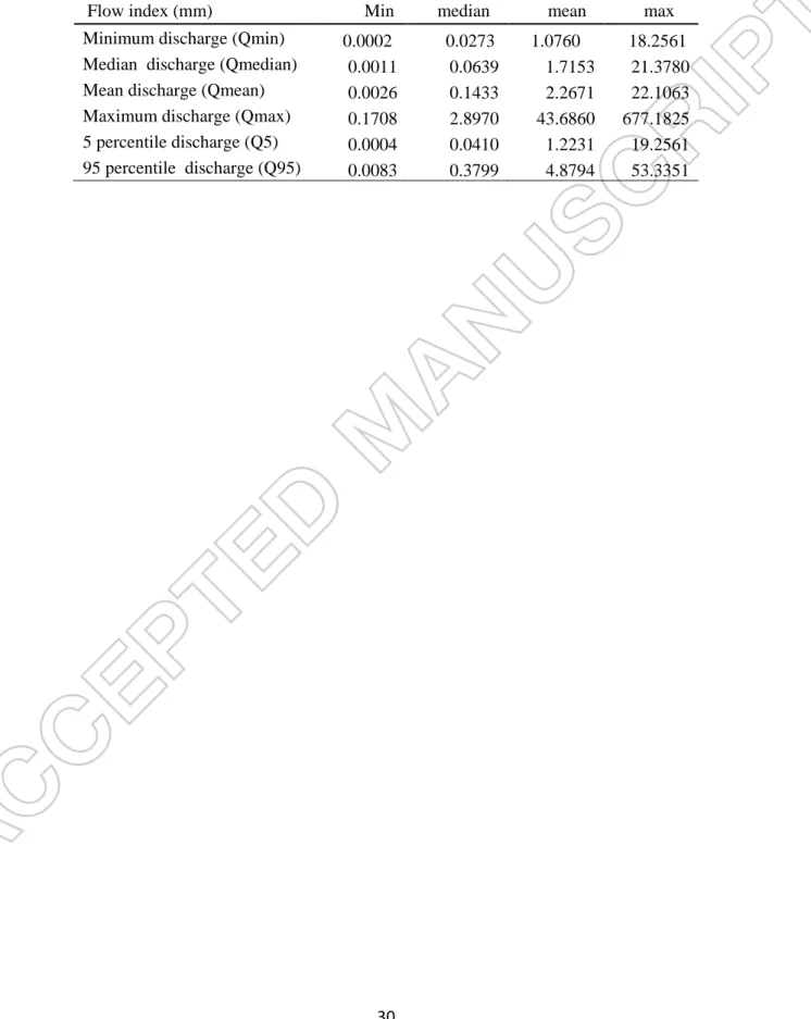
by Cheng et al. (2012) and used AP clustering on these two parameters. In this study, the mean and (0, 5, 50, 95,100) percentiles of flow are used as flow indices as suggested by Ali et al. (2012). Catchment properties used in this study are described in Section 3.1.

𝑓(𝑥; 𝛼, 𝛿) =𝛿𝛼𝑥_Γ𝛼−1_(𝛼) 𝑒−𝑥𝛿 𝑓𝑜𝑟 𝑥 ≥ 0 𝑎𝑛𝑑 𝛼, 𝛿 > 0 (5)

2.4 Catchment cluster comparison

To measure the similarity or the agreement between two clustering results we used the Adjusted Rand Index (ARI) following Ali et al. (2012). The ARI can yield a value between -1 and +1. ARI equal to 1 means complete agreement between two clustering results whereas

13

ARI equal to -1 mean a no agreement between two clustering results. The formulation of ARI (Hubert and Arabie 1985, Rand 1971) is given by:

𝐴𝑅𝐼 =

2�∑ �𝑖 𝑎𝑖2� + ∑ �𝑗 𝑏𝑗2�� − �∑ �𝑖 𝑎𝑖2� ∑ �𝑗 𝑏𝑗2�� �� 𝑛𝑖𝑗2 �

(6)

where 𝑛_𝑖𝑗, 𝑎_𝑖, 𝑏_𝑗 are values from the contingency table. If we have two groups, G1 =

{C1,C2,…, Cr} and G2= {D1, D2,..., Ds}, the overlap between G1 and G2 can be given by

contingency table [𝑛_𝑖𝑗] where each entry 𝑛_𝑖𝑗 denotes the number of objects in common

between G1 and G2. In term of hydrology, G1 and G2 are two cluster sets obtained by two different methods based on the same set of catchments. Hence, the Contingency table show how many catchments are in common between the different clustering techniques. A more

detailed example can be seen in Hubert and Arabie, (1985). The value of 𝑎_𝑖, 𝑏_𝑗 can be

obtained from table as follow: 𝑎_𝑖 = ∑𝑠_𝑗=1𝑛_𝑖𝑗 and 𝑏_𝑗 = ∑𝑟_𝑖=1𝑛_𝑖𝑗. If the clustering based on

two or more descriptor types is similar, that will improve our confidence in the methods to provide a hydrologically consistent region delineation.

2.5 Use of clustering to transfer model parameters

Once the hydrological grouping was defined, a physically based hydrological model (TopNet) was set up for all the catchments, and model parameters were individually calibrated using the Robust Parameter Estimation (ROPE) algorithm (Bárdossy and Singh 2008). To compare the transferred model parameter performance with optimal calibrated NS of the catchment, the calibrated model parameters of exemplars were transferred to the other catchments within the group. To test the usefulness of our proposed clustering measure in parameter regionalisation, we compared model performance for parameters transferred within the group versus outside the group. This represents a fair comparison because parameters for in-group and out-group catchments are both tested in validation rather than calibration model.

14

If our method is successful, we expect in-group performance to exceed out-group performance.

3 Case Study

The proposed methods of catchment clustering were tested in the Bay of Plenty (BOP) region which is located in the North Island of New Zealand.

3.1 Study Area

The study area consists of small to medium sized catchments in the BOP region (Figure 5). We selected 21 catchments for which flow data are available. Catchment area varies from 2

to 2883 km2. Each catchment is a collection of sub-basins, defined by third orders stream in

the Strahler classification. Table 1 gives the details of the 21 catchments and their properties (average over all sub-basins). These catchments are characterised by different topography, geology, soil type and land use. All catchments are rural with only minor urbanised areas. The main land uses are agriculture, dairy and sheep farming. Hourly runoff and precipitation data from the period 1990 to 2000 were obtained from the National Institute of Water and Atmospheric Research (NIWA) and BOP Regional Council. The catchment physical and hydrological properties are derived from a variety of sources including a digital river network (Snelder and Biggs 2002), 30m Digital Elevation Model, and land cover and soils databases (Newsome et al. 2000). A summary of flow indices for all the catchments are given in Table 2.

3.2 Hydrological Model

TopNet is a semi-distributed hydrological model which simulates catchment water balance and river flow. It was developed using TOPMODEL (Beven and Kirkby 1979) concepts for parameterization of soil moisture deficit using a topographic index to model the dynamics of

15

variable source areas contributing to saturation excess runoff (Bandaragoda et al. 2004, Beven and Kirkby 1979). TopNet models a catchment as a collection of sub-watersheds, linked by a branched river network (Clark et al. 2008). Flow is routed through the river network using kinematic waves using the shock-fitting technique of Goring (1994). Modelled streamflow is generated in 3 ways:

• rain falls on a location where soil water storage equals its capacity (Saturation excess runoff')

• rain rate exceeds infiltration rate ('Hortonian runoff') • saturated zone discharge into stream (baseflow)

TopNet assumes that available soil water storage can vary within a sub-watershed because of topographic effects - valley bottoms and flat places are wetter than ridges.

TopNet can be used for a variety of applications including operational flood forecasting, water resources modelling, and climate and land-use change studies (McMillan et al. 2013). It provides a prediction of flow in each modelled reach within a catchment (Ibbitt et al. 2000). The model inputs are rainfall and temperature time series (e.g at hourly time steps, with rain from one or more locations), relative humidity, solar radiation, and maps of elevation, vegetation type, soil type and rainfall patterns. These map data are used with tables of model parameters for each soil and vegetation type, to produce initial estimates of the model parameters. A schematic representation of the model is given in Figure 6. TopNet has 31 parameters to define the hydrological processes of a catchment. Where possible, parameter values are determined from physical catchment properties; however 12 parameters typically require calibration. During calibration, TopNet model uses a spatially constant multiplier for each parameter, to adjust the parameters while retaining the relative spatial pattern obtained from the soil and vegetation data (Bandaragoda et al. 2004). This procedure is necessary in order to reduce the dimensionality of the calibration problem. In this study, we transferred the

16

calibrated multiplier from one catchment to others. The model parameters to be calibrated

and their physical meaning and ranges are given in Table 3.

4 Results

4.1 Similarity Measure

The use of flow indices and descriptions of flow dynamics requires that runoff is normalised to remove the influence of runoff magnitude before similarity measures are calculated. Following the suggestion of Ley et al. (2011), runoff is normalised by its median value to eliminate most of the influence of mean precipitation and catchment area. Normalised Flow Duration Curves (FDC) for all catchments are given in Figure 7. From this figure we can see a wide range of runoff distributions. In order to summarise and compare FDCs we fitted gamma distributions (Cheng et al. 2012) with two parameters (shape and rate) for each FDC. Based on the parameters, we used the AP clustering to group the catchments. As a result of cluster analysis we obtained 6 clusters (Table 4). Groups 2, 3, 4 and 5 have only one member, which can occur when flow exceedance probabilities of these catchments are significantly different from the others (Figure 7).

DD-plots were prepared for all possible pairs of catchments. Example of DD-plots for dissimilar catchments and similar catchment are given in Figure 8. We calculated the area of the convex hull of the DD-plots and used the area to define the similarity matrix for AP clustering. Based on the DD-plots we found 6 clusters (Table 4), where group 2, 4, 5 and 6 have only one member. We calculated the flow indices for all catchments (Table 2). AP cluster analysis gave 6 clusters, four of these clusters have only one member. Catchments were also classified using a similarity measure based on catchment characteristics (as given in Table 1; the results are given in Table 4. We obtained 4 clusters, in contrast to the other similarity measures which give 6 clusters.

17

Figure 9 shows the cluster dendrogram resulting from DD-plots, FDC, flow indices and catchment properties. A dendrogram is a tree-like diagram that records the sequences of merges or splits of the clusters. The vertical axis on the dendrogram shows the level of fusion of different clusters. The heights of the merges in the dendrogram correspond to the merging objective: the higher the vertical bar of a merge, the less similar the two clusters were (Bodenhofer et al. 2012). From these figure we can see how clusters are grouped and how distinct the groups are from each other. Clustering based on flow indices gave several groups with single members. This may indicate a lack of discriminatory power in the flow indices selected. The height of the merges in the dendrogram in Figure 9 varies according to the variable used for clustering. In the case of the clustering based on DD-plots, clusters 3 and 4 as well as cluster 1 and 5 are relatively similar to each other. But clusters 2 and 6 are outliers which are dissimilar to the other four. The dendrogram based on FDC clustering show that, clusters 1 and 2 and cluster 3, 4 and 6 are relatively similar to each other, whereas cluster 5 is very dissimilar to the other five. For of clustering based on flow indices, the cluster 1, 3, 4 as well as cluster 2, 6 are very similar to each other but cluster 5 is dissimilar. For clustering based on catchment characteristics, clusters 1 and 3 are similar to each other, cluster 4 is very dissimilar to the other three. Based on each cluster we can define one hydrological parameter set.

Figure 10 shows maps of the hydrogeological permeability class along with groups derived from each of the four similarity measures. There is a clear distinction between Eastern and Western catchments in term of permeability which experience shows is a key determinant of hydrological response. Eastern catchments have low permeability compared to Western catchments. Even though some of Eastern and Western catchments are in same group, clustering based on DD-plot similarity has largely classified the Eastern and Western catchments in to different groups. Similarly, grouping of catchment based on flow statistics

18

have also grouped the Eastern and Western catchments differently. But grouping based on FDC or catchment characteristics fails to do so.

To measure the similarity or agreement between clusters based on different similarity metrics we calculated the ARI (Table 5). All four clustering methods produce dissimilar clusters as shown by low ARI values in all cases. The most similar clusters are those of the FDC and physical catchment characteristics. This contrasts with results from the previous study by Ali et al. (2012) which found that clustering based on physical catchment descriptors and flow-based indices are different. The most dissimilar clusters are those between DD-plot and physical catchment characteristics or flow-based indices. In later case, this may be due to the fact that DD-plot-based clustering uses the whole time series whereas flow indices are a summary measure.

The major advantage of using DD-plots for defining similarity of catchment over other techniques is that DD-plots enable us to use the whole time series instead of using statistics of the series. This captures the whole dynamics of the series, while allowing us to visualize the results in 2D. However, there is still a requirement to compress this information to a single value (i.e. the area of convex hull) before use as similarity measure.

In the next section, we test DD-plot based clustering for defining groups to guide model parameter transfer.

4.2 Similarity measure to guide model parameter transfer

The TopNet model was set up for all the 21 catchments. The model was calibrated for each catchment using the ROPE algorithm (Bárdossy and Singh 2008) with the Nash-Sutcliffe (NS) coefficient (Nash and Sutcliffe 1970) as the objective function with an hourly time step. The model was calibrated on one year of data with one year of warm up period. Selection of the calibration period required continuous data availability including high and low flow

19

periods. The major advantage of the ROPE algorithm based calibration is that instead of a single best parameter set it gives the convex hull of the optimal parameter space, which can account for uncertainty associated with parameter estimation. The deepest parameters in the convex hull are optimal. The resulting optimal performance score (NS) from the deepest parameter set, varied from 0.41 to 0.89 (Table 4) across different catchments. Some of the catchments have poor performance even after calibration: we hypothesise that this is due to geological characteristics of the catchments which are not properly represented by the model. Figure 11 shows model performance along with the hydrogeological classes of each catchment. From the figure, we can see that neighbouring catchments may have very different hydrogeological classes, meaning different permeability. In general the best results were obtained in larger catchments and in the East of the region, while poorer performance was obtained in small catchments draining into Tauranga Harbour in the West of the region. An hourly observed and model hydrograph and flow duration curve for the calibration time period for catchment number (station No). 13805 is given in Figure 12 and 13 resepectively, where model performance score (NS) is an average (0.71). From the figure one can see that both the hydrographs have very similar dynamics. Timing and magnitude are very similar in the observed and model hydrographs but a few very high floods were missed by the model.

To see the behaviours of the model parameters in all the catchments, we made scatter plots of the two most sensitive parameters of TopNet model, topmodf (TOPMODEL f parameter) and hydcon0 (saturated hydraulic conductivity), marked according to the groups obtained by each clustering measure (Figure 14). Parameters of the TopNet model for catchments in the same group are clustered together only for a few cases, suggesting that model behaviour is governed by the whole parameter set rather than individual parameters.

The calibrated model parameters were transferred (1) to other catchments within the same

cluster and (2) to catchments outside the cluster. The transferred parameter results were

20

compared with the performance obtained during the calibration of the catchment. To see an overview of transfer of parameters from within group and outside the group, we plotted a performance matrix of parameters transferred from each catchment to each other catchment (Figure 15). This performance matrix gives a visual indication that parameter transfer within the group typically out-performed parameter outside the group. To quantify this difference, performance statistics for transfer of parameters within and outside the group are given in Table 6 (with exemplar catchments highlighted). When using exemplar catchment parameters, mean in-group performance (NS score of -0.03) is significantly higher than out-of-group performance (NS score of -20.8). Table 6 also shows that exemplars give better parameter transfer performance than other group members, demonstrating their usefulness as representative catchments. However, we note that transfer of complete parameter sets even within groups often results in poor performance. This is because these catchments are grouped together but still they may have very diverse behaviours.

We tested the transferability of parameters between in-group and out-group catchments for the other clustering schemes, and results are given in Table 7. Results from this table again shows consistently that inside group results are better than outside group results. When using exemplar catchment parameters, mean ingroup performance in term of NS score are 0.36, -1.27, and -5.86 respectively for FDC, flow indices and catchment characteristics based clustering. Whereas outofgroup performance in term of NS score are 6.73, 42.80, and -16.53 respectively for FDC, flow indices and catchment characteristics based clustering. The results show that the DD-plot method gives the highest in-group performance scores. This demonstrates a greater hydrological consistency and more representative exemplar than other methods. The DD-plot method also gives the second-highest difference between in-group and out-group mean scores (flow indices give the highest). This demonstrates good differentiation of hydrological behaviour between clusters.

21

Figure 16 shows one example of observed and model hydrographs when parameters from catchment with station No. 15412 transferred to an out-of-group dissimilar catchment with station reach No.15514 against an in-group similar catchment with station No. 15410. From this figure one can see that in this case, within-group parameter transfer performed better than without-group transfer. However larger datasets would be need in order to generalise these results.

5 Discussion

We propose in this article a new non-parametric measure of similarity among catchments, using a data depth function which uses the whole observed time series. This new DD-Plot based approach has major advantage that there is not decision process aside from the initial parameter of data dimension (d=4). In this study we tested catchment clustering based on the following variables: (1) DD-plots based on discharge, (2) flow duration curve indices, (3) flow indices, (4) and catchment properties. The comparison among the clustering based on different methods suggest that they produce different number and members of clusters. The ARI based analysis shows that the DD-plot method produces clusters that are most dissimilar to the other methods, whereas the FDC based method and the catchment properties method produce the most similar cluster. Whereas in a previous study, Ali et al. (2012) found a clear distinction between the clustering based on physical catchment descriptors and flow-based indices. Difference in clustering based on our proposed depth-depth measure, catchment characteristics, flow, and flow indices may be due to fact that catchment characteristics used in this present study may not be very appropriate to represent all the process in the catchments. At the same time DD-plot is using the whole time series which was not used in Ali et al. (2012) studies.

22

Model performance during transfer of parameters from one catchment to other can vary widely based on both the method of regionalisation and the number of catchments used in the study (Parajka et al. (2013)). Hence, it is hard to generalise or compare the results of the various clustering technique present in this study, as the numbers of clusters and the numbers of catchments in each cluster varies from one clustering technique to other. The clustering analyses completed with the flow indices or the physical characteristics is dependent on the selection of those characteristics. Conclusions can be made on the comparison between these physical and flow characteristics, but it should be noted that comparisons between physical and flow characteristics should not be generalized to all flow and physical characteristics. One of the benefits of using the DD-Plot approach is that there is not decision process aside from the initial parameter (d=4).

Based on the current study, when exemplar catchment parameters are transferred to other catchments, the mean in-group performance in term of NS score is significantly higher than out-of-group performance in all the four clustering techniques. But the DD-plot based clustering outperform (highest in-group performance scores and second-highest difference between in-group and out-group mean scores) the other clustering methods. The second best results are from the FDC based clustering, followed by Flow indices and catchment characteristics based clustering. This suggest flow based clustering is more representative of the rainfall-runoff response of the catchments then the catchment characteristics. The reason that DD-plot based clustering outperformed the other methods may be that it takes into account the whole time series and may better present the processes of the catchments. Even though DD-plot based, transferred parameters have outperformed the other methods, the performance in term of NS is still poor. Several reasons may account for this especially that these model performance tests are in “validation” rather than “calibration” mode. The uncertainty in the locally estimated model parameters is a function of their importance in

23

representing the response of a given catchment, but the model structural error hinders identification of a parameter to represent a certain process and therefore hinders the regionalization (Wagener and Wheater 2006). Model calibration can lead to non-unique sets of parameters and therefore it can be difficult to associate parameter values with catchment characteristics, and hence to transfer them to ungauged catchments (Bárdossy 2007). Hence, there is chain of uncertainty that propagates when we transfer the parameters between catchments.

6 Conclusion

The aim of this study was to explore a new measure of similarity among catchments, using the data depth function. This is a new, non-parametric method of catchment clustering based on a measurement of the centrality of an observation within a distribution of points. We compare this new measure with existing catchment clustering metrics, i.e. flow duration curves, flow indexes and physical catchment characteristics. A cluster analysis was

performed with each of these similarity measures, using the AP clustering algorithm, and the

results were compared. We evaluated whether a similarity measure based on data depth-depth plot provides a better basis for transferring parameter sets of a hydrological model between catchments. In this study, we focused on 21 catchments located in the Bay of Plenty region in the North Island of New Zealand. The catchments have a wide range of topographic properties, response behaviours and geological features. Results show that clustering based on our proposed depth-depth measure is dissimilar to clustering based on catchment characteristics, flow, or flow indices. The TopNet model was calibrated for all the catchments and transferability of model parameters among the similar catchments was tested by transferring the parameters from within each cluster group to catchments inside and outside the group. We found that on an average, parameter transfer within the group performed

24

significantly better than outside the group. Average performance (in term of NS score) from the parameters of exemplars catchments transferred within the group have better performance than non-exemplar catchments demonstrating the usefulness of the exemplars as representation of the catchment group. The DD-plots based method was found to be a better basis for the transfer of parameter sets as compared to the other methods, bacuse it gave the best model performance for in-group catchments. This results suggest that DD-plot similarity measure outperform the other measures we tested in creating clusters of catchments with similar rainfall-runoff responses.

Acknowledgment

The authors wish to thank Bay of Plenty Regional Council for providing flow data for this study. The authors would like to thanks editor Alberto Viglione for handling the article and positive comments. The authors gratefully acknowdge the detailed and constractive comments made by Juraj Parajka and two anonymous reviewer which greatly helped improve this article.

Funding

This work was funded by the New Zealand Ministry of Science and Innovation, Contract number C01X0812.

25 References

Ali, G., Tetzlaff, D., Soulsby, C., McDonnell, J.J., Capell, R., 2012. A comparison of similarity indices for catchment classification using a cross-regional dataset. Advances in Water Resources, 40: 11-22.

Andrew, Y.C., Regina, Y., James, T.L., 2000. Monitoring multivariate aviation safety data by data depth: control charts and threshold systems. IIE Transactions, 32(9): 861-872. Bandaragoda, C., Tarboton, D.G., Woods, R., 2004. Application of TOPNET in the

distributed model intercomparison project. Journal of Hydrology, 298(1-4): 178-201. Bárdossy, A., 2007. Calibration of hydrological model parameters for ungauged catchments.

Hydrology and Earth System Sciences Discussions, 11(2): 703-710.

Bardossy, A., Singh, S.K., 2011. Regionalization of hydrological model parameters using data depth. Hydrology Research, 42(5): 356-371.

Bárdossy, A., Singh, S.K., 2008. Robust estimation of hydrological model parameters. Hydrology and Earth System Sciences, 12: 1273-1283.

Barnett, V., 1976. The ordering of multivariate data (with discussion). Journal of Royal Statistical Society A, 139: 318-354.

Beven, K., Kirkby, M., 1979. A physically based, variable contributing area model of basin hydrology/Un modèle à base physique de zone d'appel variable de l'hydrologie du bassin versant. Hydrological Sciences Journal, 24(1): 43-69.

Beven, K.J., 2004. Rainfall-runoff modelling: the primer. Wiley.

Blöschl, G., 2005. Rainfall‐Runoff Modeling of Ungauged Catchments. Encyclopedia of

Hydrological Sciences.

Bodenhofer, U., Kothmeier, A., Bodenhofer, M.U., 2012. Package ‘apcluster’.

Chebana, F., Ouarda, T., 2008. Depth and homogeneity in regional flood frequency analysis. Water Resources Research, 44(11): W11422.

Chebana, F., Ouarda, T., 2011a. Multivariate quantiles in hydrological frequency analysis. Environmetrics, 22(1): 63-78.

Chebana, F., Ouarda, T.B.M.J., 2011b. Depth-based multivariate descriptive statistics with hydrological applications. J Geophys Res-Atmos, 116(D10120): D10120.

Chebana, F., Ouarda, T.B.M.J., 2011c. Multivariate extreme value identification using depth functions. Environmetrics, 22(3): 441-455.

Cheng, L., Yaeger, M., Viglione, A., Coopersmith, E., Ye, S., Sivapalan, M., 2012. Exploring the physical controls of regional patterns of flow duration curves–Part 1: Insights from statistical analyses. Hydrol. Earth Syst. Sci. Discuss, 9: 7001-7034.

Clark, M.P., Rupp, D.E., Woods, R.A., Zheng, X., Ibbitt, R.P., Slater, A.G., Schmidt, J., Uddstrom, M.J., 2008. Hydrological data assimilation with the ensemble Kalman filter: Use of streamflow observations to update states in a distributed hydrological model. Advances in Water Resources, 31(10): 1309-1324.

Dutta, S., Ghosh, A.K., 2012. On robust classification using projection depth. Annals of the Institute of Statistical Mathematics, 64(3): 657-676.

Frey, B.J., Dueck, D., 2007. Clustering by passing messages between data points. science, 315(5814): 972-976.

Goring, D.G., 1994. Kinematic shocks and monoclinal waves in the Waimakariri, a steep, braided, gravel-bed river, Proceedings of the International Symposium on Waves: Physical and Numerical Modelling. University of British Columbia, Vancouver, Canada, pp. 336-345.

Guerrero, J.L., Westerberg, I.K., Halldin, S., Lundin, L.C., Xu, C.Y., 2013. Exploring the

hydrological robustness of model‐parameter values with alpha shapes. Water

Resources Research, 49(10): 6700-6715.

26

Hamurkaroglu, C., Mert, M., Saykan, Y., 2006. Nonparametric control charts based on Mahalanobis depth. QUALITY CONTROL AND APPLIED STATISTICS, 51(1): 21. He, Y., Bárdossy, A., Zehe, E., 2011. A catchment classification scheme using local variance

reduction method. Journal of Hydrology 411(1-2):140-154.

Hrachowitz, M., Savenije, H.H.G., Blöschl, G., McDonnell, J.J., Sivapalan, M., Pomeroy, J.W., Arheimer, B., Blume, T., Clark, M.P., Ehret, U., 2013. A decade of Predictions in Ungauged Basins (PUB)—a review. Hydrological sciences journal, 58(6): 1198-1255.

Hubert, L., Arabie, P., 1985. Comparing partitions. Journal of classification, 2(1): 193-218. Ibbitt, R.P., Henderson, R.D., Copeland, J., Wratt, D.S., 2000. Simulating mountain runoff

with meso-scale weather model rainfall estimates: a New Zealand experience. Journal of Hydrology, 239(1–4): 19-32.

Krauße, T., Cullmann, J., 2009. Towards robust estimation of hydrological parameters focusing on flood forecasting in small catchments, 18th World IMACS / MODSIM Congress, Cairns, Australia.

Ley, R., Casper, M., Hellebrand, H., Merz, R., 2011. Catchment classification by runoff behaviour with self-organizing maps (SOM). Hydrology and Earth System Sciences, 15(9): 2947.

Li, J., Cuesta-Albertos, J.A., Liu, R.Y., 2012. DD-classifier: Nonparametric classification procedure based on DD-plot. Journal of the American Statistical Association, 107(498): 737-753.

Liu, R., 1976. On a notion of data depth based on random simplices. Annals of Statistics, 18: 405-414.

Liu, R.Y., 1995. Control charts for multivariate processes. Journal of the American Statistical Association, 90(432): 1380-1387.

Liu, R.Y., Parelius, J.M., Singh, K., 1999. Multivariate analysis by data depth: descriptive statistics, graphics and inference,(with discussion and a rejoinder by Liu and Singh). The Annals of Statistics, 27(3): 783-858.

Liu, R.Y., Serfling, R.J., Souvaine, D.L., 2006. Data depth: robust multivariate analysis, computational geometry, and applications, 72. Amer Mathematical Society.

Liu, R.Y., Singh, K., 1993. A quality index based on data depth and multivariate rank tests. Journal of the American Statistical Association: 252-260.

McDonnell, J.J., Woods, R., 2004. On the need for catchment classification. Journal of Hydrology(Amsterdam), 299(1): 2-3.

McMillan, H., Hreinsson, E., Clark, M., Singh, S., Zammit, C., Uddstrom, M., 2013. Operational hydrological data assimilation with the recursive ensemble Kalman filter. Hydrology and Earth System Sciences, 17: 21-38.

Merz, R., Blöschl, G., 2004. Regionalisation of catchment model parameters. Journal of Hydrology, 287(1): 95-123.

Messaoud, A., Weihs, C., Hering, F., 2004. A Nonparametric Multivariate Control Chart Based on Data Depth, Technical Report/Universität Dortmund, SFB 475 Komplexitätsreduktion in Multivariaten Datenstrukturen.

Nash, J.E., Sutcliffe, J., 1970. River flow forecasting through conceptual models part I—A discussion of principles. Journal of Hydrology, 10(3): 282-290.

Newsome, P.F.J., Wilde, R.H., Willoughby, E.J., 2000. Land Resource Information System Spatial Data Layers. Landcare Research Technical Report No.84p

Parajka, J., Merz, R., Blöschl, G., 2005. A comparison of regionalisation methods for catchment model parameters. Hydrology and Earth System Sciences Discussions Discussions, 2(2): 509-542.

27

Parajka, J., Viglione, A., Rogger, M., Salinas, J. L., Sivapalan, M., and Blöschl, G. 2013. Comparative assessment of predictions in ungauged basins – Part 1: Runoff-hydrograph studies, Hydrol. Earth Syst. Sci., 17, 1783-1795

Post, D.A., Jakeman, A.J., 1999. Predicting the daily streamflow of ungauged catchments in SE Australia by regionalising the parameters of a lumped conceptual rainfall-runoff model. Ecological Modelling, 123(2): 91-104.

Rand, W.M., 1971. Objective Criteria for the Evaluation of Clustering Methods. Journal of the American Statistical Association, 66(336): 846-850.

Razavi, T., Coulibaly, P., 2013. Classification of Ontario watersheds based on physical attributes and streamflow series. Journal of Hydrology, 493(0): 81-94.

Rousseeuw, P.J., Struyf, A., 1998. Computing location depth and regression depth in higher dimensions. Statistics and Computing, 8(3): 193-203.

Salinas, J. L., Laaha, G., Rogger, M., Parajka, J., Viglione, A., Sivapalan, M., and Blöschl, G.2013. Comparative assessment of predictions in ungauged basins – Part 2: Flood and low flow studies, Hydrol. Earth Syst. Sci., 17, 2637-2652.

Samaniego, L., Bárdossy, A., Kumar, R., 2010. Streamflow prediction in ungauged catchments using copula-based dissimilarity measures. Water Resources Research, 46(2): W02506.

Sawicz, K., Wagener, T., Sivapalan, M., Troch, P. A., and Carrillo, G. 2011. Catchment classification: empirical analysis of hydrologic similarity based on catchment function in the eastern USA, Hydrol. Earth Syst. Sci., 15, 2895-2911

Serfling, R., 2002. Generalized quantile processes based on multivariate depth functions, with applications in nonparametric multivariate analysis. Journal of Multivariate Analysis, 83(1): 232-247.

Singh, S.K., Bárdossy, A., 2012. Calibration of hydrological models on hydrologically unusual events. Advance in Water Resources, 38(0): 81-91.

Singh, S.K., McMillan, H., Bárdossy, A., 2013. Use of the data depth function to differentiate between case of interpolation and extrapolation in hydrological model prediction. Journal of Hydrology, 477: 213-228.

Sivapalan, M., Takeuchi, K., Franks, S., Gupta, V., Karambiri, H., Lakshmi, V., Liang, X., McDonnell, J., Mendiondo, E., O'connell, P., 2003. IAHS Decade on Predictions in Ungauged Basins (PUB), 2003–2012: Shaping an exciting future for the hydrological sciences. Hydrological Sciences Journal, 48(6): 857-880.

Snelder, T.H., Biggs, B.J.F., 2002. Multiscale River Environment Classification for water resources Managements1. JAWRA Journal of the American Water Resources Association, 38(5): 1225-1239.

Stoumbos, Z.G., Jones, L.A., Woodall, W.H., Reynolds, M., 2001. On nonparametric multivariate control charts based on data depth. Frontiers in Statistical Quality Control 6, 6: 207.

Toth, E. 2013. Catchmnet classification based on characterion of stream and precipiation time series. Hydrol. Earth Syst. Sci., 17: 1149-1159.

Tukey, J., 1975. Mathematics and picturing data. In Proceedings of the International 17 Congress of Mathematics, 2: 523-531.

Viglione, A., Parajka, J., Rogger, M., Salinas, J. L., Laaha, G., Sivapalan, M., and Blöschl, G.: Comparative assessment of predictions in ungauged basins – Part 3: Runoff signatures in Austria, Hydrol. Earth Syst. Sci., 17, 2263-2279, doi:10.5194/hess-17-2263-2013, 2013.

Vogel, R.M., 2006. Regional calibration of watershed models. Watershed Models, 1: 47-71. Wagener, T., Sivapalan, M., Troch, P., Woods, R., 2007. Catchment classification and

hydrologic similarity. Geography Compass, 1(4): 901-931.

28

Wagener, T., Wheater, H., Gupta, H.V., 2004. Rainfall-runoff modelling in gauged and ungauged catchments. World Scientific Publishing Company.

Wagener, T., Wheater, H.S., 2006. Parameter estimation and regionalization for continuous rainfall-runoff models including uncertainty. Journal of hydrology, 320(1): 132-154.

Wazneh, H., Chebana, F., Ouarda, T., 2013a. Depth‐based regional index‐flood model. Water

Resources Research, 49(12): 7957-7972.

Wazneh, H., Chebana, F., Ouarda, T.B.M.J., 2013b. Optimal depth-based regional frequency analysis. Hydrol. Earth Syst. Sci., 17(6): 2281-2296.

Zuo, Y., Serfling, R., 2000. General notions of statistical depth function. The Annals of Statistics, 28(2): 461-482.

29

Table 1 Catchment properties (averaged over sub-basins). The minimum and maximum elevation is in metres above mean sea level (m a.m.s.l.). Permeability, 1: very low, 2: low, 3: medium, 4: high medium, 5: high, 6: medium high, 7: very high.

Station no. Area (km2) Average length of stream reach (m) Average width of stream reach (m) Average ln(a/tan(² ) ) Minimum elevation of stream reach (m a.m.s.l.) Maximum elevation of stream reach (m a.m.s.l.) Average gradient of stream reach (-) Catchment averaged permeability 17101 348.8 3906.8 10.1 7.4 6.2 717.7 0.0294 1 13805 9.5 3999.0 4.6 9.1 220.7 300.3 0.0198 5 13310 37.9 1880.0 6.1 7.2 39.1 284.3 0.0192 5 14410 59.7 4280.6 7.1 8.7 19.1 284.0 0.0176 6 15341 186.9 2244.4 6.2 8.0 298.6 557.6 0.0275 7 14130 295.2 2742.8 7.9 8.1 20.0 500.7 0.0258 6 15410 507.4 2582.5 10.0 7.8 199.6 827.6 0.0216 6 15412 2882.9 3060.1 16.7 8.5 5.0 827.6 0.0174 6 15450 154.2 2820.0 7.9 8.3 203.5 498.8 0.0311 5 16502 294.2 2691.2 9.7 7.8 427.0 632.2 0.0121 3 15901 660.4 3041.9 10.9 7.5 63.5 801.9 0.0335 4 1114651 51.9 3226.6 7.0 8.4 4.6 177.7 0.0113 6 15605 67.6 2401.8 6.8 8.4 21.9 59.3 0.0046 5 15544 214.4 3175.1 8.7 7.6 120.9 644.1 0.0359 5 16002 239.8 3486.6 9.2 7.7 26.7 457.8 0.0230 2 15302 700.9 2649.1 10.7 8.4 0.1 557.6 0.0220 7 15408 1149.7 3146.9 12.1 8.9 184.0 820.0 0.0121 7 16501 1377.1 3280.6 13.3 7.5 12.9 826.9 0.0266 3 15514 1485.0 1793.0 2.3 7.1 12.0 16.8 0.0026 5 13901 2.9 1164.0 2.5 9.3 19.0 34.5 0.0134 7 15472 110.2 2604.8 7.8 8.4 301.8 498.8 0.0171 6

30

Table 2 Summary of flow indices (mm) used in this study

Flow index (mm) Min median mean max Minimum discharge (Qmin) 0.0002 0.0273 1.0760 18.2561 Median discharge (Qmedian) 0.0011 0.0639 1.7153 21.3780 Mean discharge (Qmean) 0.0026 0.1433 2.2671 22.1063 Maximum discharge (Qmax) 0.1708 2.8970 43.6860 677.1825 5 percentile discharge (Q5) _{0.0004 0.0410 1.2231 19.2561} 95 percentile discharge (Q95) _{0.0083 0.3799 4.8794 53.3351}

31

Table 3 Model parameters of the TopNet which need calibration, description and allowed range for the

parameter multiplier Parameter Description Initial Min Max

topmodf TOPMODEL f parameter (m-1) 0.001 2

hydcon0 Saturated hydraulic conductivity (m s-1) 0.01 9999

swater1 Drainable water (m) 0.05 20

swater2 Plant-available water (m) 0.05 20

dthetat Soil water content (m) 0.1 10

overvel Overland flow velocity (m s-1) 0.1 10

gucatch Gauge under-catch for snowfall (-) 0.5 1.5

th_accm Threshold for snow accumulation (K) 272.16 275.16

th_melt Threshold for snowmelt (K) 272.16 275.16

snowddf Mean degree-day factor for snowmelt (mm K

-1

d-1 = kg m-2

K-1 d-1) 0.1 7.5

minddfd Minimum degree-day-factor day (Julian day: 1 to 366) 1 366

maxddfd Maximum degree-day-factor day (Julian day: 1 to 366) 1 366

snowamp Seasonal amplitude of degree-day factor for snowmelt (mm

K-1 d-1 = kg m-2 K-1 d-1) 0 7.5

cv_snow Coefficient of variation in sub-grid SWE (-) 0.5 1.5

r_man_n Manning’s n (-) 0.1 10

32

Table 4 Calibration results for all the catchments and catchments group based on clustering on flow and

catchment characteristics (bold number are exemplars)

Station Station

DD plot FDC _indices Flow _{characteristics} Catchment

no. name NS 17101 Raukokore at SH35 Br 0.69 1 6 3 3 13805 Waipapa at Goodall Rd 0.71 1 6 3 3 13310 Tuapiro at Woodlands Rd 0.65 1 6 1 3 14410 Waimapu at McCarrolls 0.77 1 6 4 3

15341 Tarawera at Lake Outlet Recorder 0.79 1 2 4 3

14130 Wairoa at Above Ruahihi 0.64 1 6 2 3

15410 Whirinaki at Galatea 0.7 1 6 3 1

15412 Rangitaiki at Te Teko 0.81 1 4 3 4

15450 Pokairoa at Railway Culvert 0.41 2 1 3 3

16502 Motu at Waitangirua 0.8 3 6 3 3

15901 Waioeka at Gorge Cableway 0.86 3 6 3 1

1114651 Raparapahoe at Above Drop Structure 0.63 3 6 4 3

15605 Nukuhou at Old Quarry 0.89 3 6 3 3

15544 Waimana at Ranger Station 0.63 3 6 4 3

16002 Otara at Browns Br 0.8 3 6 3 3 15302 Tarawera at Awakaponga 0.79 3 1 4 1 15408 Rangitaiki at Murupara 0.88 3 3 4 2 16501 Motu at Houpoto 0.73 3 6 4 2 15514 Whakatane at Whakatane 0.84 4 6 3 2 13901 Mangawhai at Omokoroa 0.69 5 6 5 3 15472 Mangaharakeke at Parapara Rd 0.58 6 5 6 3

33

Table 5 Adjusted rand index (ARI) for different clustering (ARI = –1: worse, ARI = 1: best agreement between

two clusters). DD-plot FDC Flow indices Catchment characteristics DD-plot 1 FDC _0.070 1 Flow indices _{-0.025 0.012} 1 Catchment characteristics _{-0.050 0.153 0.056} 1

Table 6 Statistics (in term of NS) of transfer of parameters of all catchments within the group and outside the

group based on DD-plot based clustering (bold number are exemplars)

Station Within group (NS) Outside group(NS)

no. Min Median Mean Max Min Median Mean Max

Group 1 17101 -18.68 -0.09 -2.73 0.35 -559.31 -1.62 -73.33 0.83 13805 -80.98 -2.49 -13.49 0.65 -1694.40 -3.48 -237.57 0.40 13310 -78.39 -2.09 -12.74 0.36 -2094.09 -2.66 -252.68 0.63 14410 -8.63 0.21 -1.01 0.64 -182.82 0.45 -26.04 0.77 15341 -0.06 -0.03 0 0.14 -51.58 0.00 -7.00 0.79 14130 -25.67 0.31 -3.76 0.58 -243.37 0.22 -35.48 0.71 15410 -0.92 -0.01 -0.05 0.39 -98.18 0.27 -14.56 0.88 15412 -15.06 0.1 -2 0.7 -73.86 0.15 -12.46 0.32 Group 2 15450 0.41 0.41 0.41 0.41 -5.07 -0.03 -0.30 0.81 Group 3 16502 -536.67 -5.07 -74.49 0.73 -3147.35 -6.91 -443.67 0.43 15901 -45.25 0.32 -5.76 0.89 -483.27 -0.16 -62.09 0.67 1114651 -18.22 0.65 -2.04 0.78 -67.27 0.05 -9.80 0.72 15605 -210.39 0.36 -28.1 0.77 -1113.43 -1.92 -160.44 0.36 15544 -55.31 -0.56 -8.02 0.58 -165.67 -0.08 -25.26 0.84 16002 -107.71 0.42 -14.71 0.86 -1467.26 -0.29 -199.86 0.67 15302 -0.21 0.02 0.11 0.58 -28.33 0.16 -3.96 0.77 15408 -0.37 0.09 0.04 0.16 -39.61 0.03 -5.80 0.79 16501 -24.12 -0.94 -3.81 0.8 -113.02 0.15 -16.16 0.74 Group 4 15514 0.84 0.84 0.84 0.84 -11.23 -0.02 -0.68 0.79 Group 5 13901 0.68 0.68 0.68 0.68 -436.10 -0.48 -43.19 0.71 Group 6 15472 0.58 0.58 0.58 0.58 -20.12 -0.11 -1.66 0.41

34

Table 7 Statistics (in term of mean NS) of transfer of parameters of all catchments within the group and outside

the group based on different clustering techniques

DD-plot FDC Flow indices Catchment

characteristics

In-group -0.03 -0.36 -1.27 -5.86

Out-group -20.80 -6.73 -42.80 -16.53

35

Figure 1 Example of a convex hull using hydrological variable discharge. The convex hull of a set of points is the smallest convex set which encloses all the points. A hyperplane is a plane passing through a

point or points. Depth measures the centrality of a point with respect to the median.

36

Figure 2 Systematic representations of similarity and dissimilarity between catchments based on convex hull of the discharge from two catchments

37

Figure 3 Example of a DD-plot (c) using 4-D (flow with lag 3) and comparison with 2-D plot (a) (flow with lag 1) and 3-D plots (b) (flow with lag 2). Flow was normalised with the median flow

(a)

(b)

(c)

38

Figure 4 Example of DD-plots (d=2) Left: using two sets of random samples from the same distribution (convex hull area: 0.043), Right: using sets of random samples from two different distributions (convex hull area: 0.082).

39

Figure 5 Study Area: Bay of Plenty region, located in North island of New Zealand

40

Figure 6 Systematic Representation of TopNet model structure

41

Figure 7 Flow duration curves for each catchment in our study. Flow was normalised by its median in each catchment

42

Figure 8 Example of DD-plots for dissimilar catchments (left) and similar catchment (right)

43

Figure 9 (a) Clustering based on flow series using area under DD-plots as similarity matrix, (b) Clustering based on flow duration curve and parameters of gamma distribution fitted for FDC, (c) Clustering based on flow indices, and (d) Clustering based on catchment characteristics

(a) (b)

(d) (c)

44

45

Figure 10 (a) groups from DD_plots clustering, (b) groups from FDC distribution parameter clustering, (c) groups from clustering from flow statistics and (d) groups from clustering based on catchment characteristics

46

Figure 11 Model performance along with different hydrogeological classes in the catchments

47

Figure 12 Hourly calibrated Observed and model hydrograph along with hyetograph for catchment with station No. 13805

48

Figure 13 Hourly calibrated Observed and model flow duration curve for catchment with station No. 13805

49

Figure 13 Plot of two important parameters of TopNet- topmodf and hydcon0 and grouped mark based on different clustering, (Top left: from DD-plot, Top right: from FDC, Bottom left: from flow indices, Bottom right: from catchment characteristics)

50

Figure 14 Performance Matrix of parameters transferred to catchment within the group and outside the group. The x axis is marked with a different box for each group. Circle show the exemplar catchment from each group. Groups where obtained from DD-plot based clustering

51

Figure 15 Observed and model hydrograph when parameter from catchment with station No. 15412 transferred to dissimilar catchment with station No. 15514 (top) and similar catchment with station No. 15410 (bottom)