HAL Id: hal-00296186
https://hal.archives-ouvertes.fr/hal-00296186
Submitted on 5 Apr 2007
HAL is a multi-disciplinary open access
archive for the deposit and dissemination of
sci-entific research documents, whether they are
pub-lished or not. The documents may come from
teaching and research institutions in France or
abroad, or from public or private research centers.
L’archive ouverte pluridisciplinaire HAL, est
destinée au dépôt et à la diffusion de documents
scientifiques de niveau recherche, publiés ou non,
émanant des établissements d’enseignement et de
recherche français ou étrangers, des laboratoires
publics ou privés.
Cloudsat configuration
A. Battaglia, M. O. Ajewole, C. Simmer
To cite this version:
A. Battaglia, M. O. Ajewole, C. Simmer. Evaluation of radar multiple scattering effects in
Cloud-sat configuration. Atmospheric Chemistry and Physics, European Geosciences Union, 2007, 7 (7),
pp.1719-1730. �hal-00296186�
www.atmos-chem-phys.net/7/1719/2007/ © Author(s) 2007. This work is licensed under a Creative Commons License.
Chemistry
and Physics
Evaluation of radar multiple scattering effects in Cloudsat
configuration
A. Battaglia1, M. O. Ajewole2, and C. Simmer3
1Meteorological Institute, University of Bonn, Bonn, Germany
2Department of Physics, Federal University of Technology, Akure, Nigeria 3Meteorological Institute, University of Bonn, Bonn, Germany
Received: 26 April 2006 – Published in Atmos. Chem. Phys. Discuss.: 28 August 2006 Revised: 30 October 2006 – Accepted: 27 March 2007 – Published: 5 April 2007
Abstract. MonteCarlo simulations have been performed to evaluate the importance of multiple scattering effects in co-and cross-polar radar returns for 94 GHz radars in Cloudsat and airborne configurations. Thousands of vertically struc-tured profiles derived from some different cloud resolving models are used as a test-bed. Mie theory is used to de-rive the single scattering properties of the atmospheric hy-drometeors. Multiple scattering effects in the co-polar chan-nel (reflectivity enhancement) are particularly elusive, espe-cially in airborne configuration. They can be quite consis-tent in satellite configurations, like CloudSat, especially in regions of high attenuation and in the presence of highly forward scattering layers associated with snow and graupel particles. When the cross polar returns are analysed [but note that CloudSat does not measure any linear depolariza-tion ratio (LDR hereafter)], high LDR values appear both in space and in airborne configurations. The LDR signatures are footprints of multiple scattering effects; although depo-larization values as high as −5 dB can be generated including non-spherical particles in single scattering modelling, multi-ple scattering computations can produce values close to com-plete depolarization (i.e. LDR=0 dB). Our simulated LDR profiles from an air-borne platform well reproduce, in a sim-ple frame, some experimental observations collected during the Wakasa Bay experiment. Since LDR instrumental uncer-tainties were not positively accounted for during that exper-iment, more focused campaigns with air-borne polarimetric radar are recommended. Multiple scattering effects can be important for CloudSat applications like rainfall and snow-fall retrievals since single scattering based algorithms will be otherwise burdened by positive biases.
Correspondence to: A. Battaglia
1 Introduction
The CloudSat mission, that will be launched early in 2006 as part of the NASA ESSP Program and of the A-train con-stellation, (Stephens et al., 2002), will fly the first space-borne millimeter wavelength radar. Among its main goals, the mission aims to detect snowfall from space, estimate how efficiently the atmosphere produces rain from conden-sates and which percentage of terrestrial clouds produce rain, and to provide statistics on the vertical structure of clouds and light rain around the globe (e.g. Stephens, 2005). In this respect, CloudSat observations can be seen as comple-mentary to those planned for companion space-borne radars (like the one to be deployed on the GPM core satellite, http: //gpm.gsfc.nasa.gov/) at lower frequencies and focused at ob-serving and profiling situations with moderate to heavy rain. Compared to GPM-like radars, the higher frequency of the CloudSat radar has the clear advantage of a better sensitiv-ity to small cloud droplets and crystals, and of lower power, weight and size. This transfers into a better spatial resolution and a lower threshold of detection. In exchange, attenuation by atmospheric gases and by hydrometeors becomes an is-sue (Lhermitte, 1987, 1990). L’Ecuyer and Stephens (2002) analyzed the importance of attenuation effects when consid-ering spaceborne radars at frequencies above 10 GHz. They implemented a very general optimal estimation-based algo-rithm for retrieving profiles of rainfall, capable of accounting for different drop size/particle shape distribution and flexible to include additional measurements from other sensors when available. When considering a 94 GHz radar, their results show that the attenuation effects are too severe to allow an ac-curate retrieval at rain rates greater than 1.5 mm/h. L’Ecuyer and Stephens (2002) concluded that only an additional con-straint of the precipitation water path can raise this limit up to 10 mm/h.
However, their retrieval methodology is based on the fun-damental assumption of the validity of the single scattering
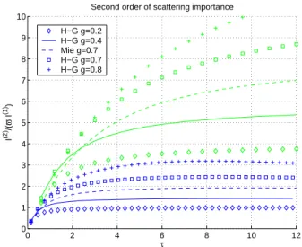
0 2 4 6 8 10 12 0 1 2 3 4 5 6 7 8 9 10
Second order of scattering importance
τ I (2) /( ϖ I (1) ) H−G g=0.2 H−G g=0.4 Mie g=0.7 H−G g=0.7 H−G g=0.8
Fig. 1. Relevance of the second order of scattering (defined as the ratio between the intensity relative the second order of scattering and the product of the SS albedo and the SS intensity) as a func-tion of the optical thickness. Blue and green lines correspond to a
uniform layer with extinction coefficient equal to 0.6 and 2.4 km−1
respectively.
(SS hereafter) approximation for the radar equation. Pre-vious studies at lower frequencies (Marzano et al., 2003; Battaglia et al., 2005; Kobayashi et al., 2005) have shown that multiple scattering (MS) effects become relevant in space-borne configuration at 35 GHz at high scattering opti-cal thickness (defined as the columnar integral of the scatter-ing coefficient), e.g. associated with large amounts of high-density ice particles. When reverting to 94 GHz the general increase of the SS albedo and of the extinction properties of all the hydrometeors will certainly favour the presence of
MS effects. For a narrow beamwidth radar system, such as
the one to be mounted on CloudSat, a further increase in the forward scattering and consequently of the g parameter also implies an increase of MS effects. On the other hand, higher frequencies allow for smaller antenna footprints (equal to 1.4×2.5 km2 for CloudSat), that will generally reduce MS effects. It is therefore the main goal of this paper to investi-gate whether or not MS effects can be relevant to the variety of applications associated with the CloudSat space-mission. Particular attention will be focused on evaluating MS effects when profiles involving snow and low rain rates are consid-ered. Strategies will be discussed that might get rid of MS-affected profiles in the retrieval procedure. Finally, the study will investigate under which conditions and in which radar signals will MS effects be revealed in air-borne field cam-paigns preliminary to the launch of CloudSat. To do this the results of our simulations will be compared with airborne ob-servations acquired during the Wakasa Bay Experiment by a CloudSat radar prototype.
2 MS effects in the radar signal
Battaglia et al. (2006a) have described a Monte Carlo-based simulator capable of evaluating single and multiple scattering apparent reflectivities for general radar configurations. Prac-tically the Monte Carlo code solves the time-dependent ra-diative transfer equation; as such, backscattered radiation is collected according to the travelled path (despite it has un-dergone single or MS) in the corresponding range-bin.
The model has been employed to simulate signals for Ku (14 GHz) and Ka (35 GHz) radars envisaged for the future GPM mission (see Battaglia et al., 2006b). Here the same tool is applied to W −band radars (94 GHz). For the space-borne configuration we will use the CloudSat parameters [altitude 705 km, beamwidth 0.1◦×0.1◦, minimum detec-tion threshold (MDT hereafter) –26 dBZ] while the airborne configurations are chosen close to those adopted for the NASA ER-2 and DC-8 cloud radars (see Li et al., 2004; Sad-owy et al., 1997) [altitude 20/6 km, beamwidth 0.8◦×0.8◦,
MDT =−40 dBZ (but it should be distance-dependent, as
shown in Fig. 4 in Li et al., 2004)]. The two airplane alti-tudes account for both stratospheric and tropospheric flights. In all cases nadir (downward-looking) radars are considered. The surface is always considered as a black surface. How-ever this is not relevant because only ranges shorter than the surface-range itself are considered hereafter. A realistic sur-face model is necessary only when the return from ranges longer than the surface-range is seeked.
2.1 Uniform layer results
The CloudSat space-borne configuration has been imple-mented first in the analytical model described in Battaglia et al. (2006a) to assess the importance of the second order of scattering (and thus indirectly of the MS) for an homoge-neous layer with a prescribed SS albedo ̟ , extinction coef-ficent kextand phase function. In the model the transmitted
radar pulse is perfectly collimated while in the receiving seg-ment the (CloudSat) antenna pattern is applied. Fig. 1 shows the ratio between the contribution of second order of scat-tering and the product of ̟ and the contribution of the first order of scattering. This quantity becomes more important with depth into the medium, with stronger extinguishing me-dia (compare the blue and the green curves) and with phase functions that are increasingly peaked (compare the differ-ent style curves). In Fig. 1 Henyey-Greenstein phase func-tions with different values of the asymmetry parameter g are considered. For instance, for a medium with an extinction coefficient equal 0.6 km−1(blue lines in Fig. 1) and a phase function with g=0.7 (0.8), at large optical thickness (right side of the panel), the second order of scattering contribu-tion is almost 2.5 (3.2) larger than for a medium with a phase function with g=0.2.
When reverting to phase functions computed with Mie the-ory the MS importance is slightly reduced. This is due to the
different details of the phase functions (see also discussion in Sect. 4.2 in Battaglia et al., 2006a), which are depicted in Fig. 2. Note in particular the presence of the backscattering peak (better to say a backscattering plateau in this case) in the Mie-computed phase function that is absent in the always decreasing Henyey-Greenstein phase function and the higher forward peak in the Henyey-Greenstein phase function.
It is relevant that at 94 GHz g values around 0.7 are eas-ily obtained in presence of ice hydrometeors when the scat-tering properties are computed with Mie theory (in combina-tion with the Maxwell and Garnett mixing rule, see chap. 8 in Bohren and Huffman, 1983). The amplitude of the g param-eter is typically enhanced when low density particles (like snow) are considered. However, some investigations of scat-tering properties of ice/snow particles, Liu (2004), have re-vealed that, when non spherical shapes are considered, lower values of the g parameter are usually obtained. As a result of the former discussion, when reverting to non-spherical shapes MS effects should be slightly reduced.
2.2 Inhomogeneous layer results
To be more realistic we have analyzed many different profiles extracted from different Cloud Resolving Models (CRM) simulations of different mesoscale systems. Six hydromete-ors are considered including uniform size cloud droplets (ra-dius 10 µm) and ice crystals (ra(ra-dius 10 µm), raindrops, grau-pel (density 0.4 g/cm3) and snow (density 0.1 g/cm3) with the latter three hydrometeor classes having exponential size distribution with a fixed intercept parameter N0. While for
rain this intercept is always equal to 1.6×10⁴m−3mm−1,
for graupel and snow this parameter is equal to 1.6×10⁴and 3.2×10⁴m−3mm−1respectively. Mixed-phase
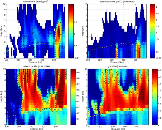
hydromete-ors are not included. For more details see Battaglia et al. (2006b). Overpasses both of a space-borne and of an air-borne W −band radar over those systems have been con-sidered. Some examples of the output of the simulator are shown in Figs. 3–4. The total hydrometeor profile (the sum of all the hydrometeor species) is depicted in the top left panel of Fig. 3 with the dashed-dotted line indicating the freezing level. The cross section is characterized by different precipitating cells consisting of a variety of rain rates at the ground resulting from a mixture of cold and warm processes. The associated SS properties are plotted in the other three panels of the same figure. Extinction coefficients as high as 4 km−1 are found in heavy precipitation areas: this
corre-sponds to a mean radiation path (the inverse of the extinc-tion coefficient) of 250 m, which is much smaller than the CloudSat footprint diameter. The SS albedo is always higher than 0.9 in the ice portion while it never exceeds 0.5 below the freezing level (indicated by the dashed-dotted line). The asymmetry parameter ranges between 0.5 and 0.8 in the ice region while it can reach values as high as 0.4 when large raindrops are present. The corresponding MS reflectivity, as sensed by W −band radars flying over the scene
character-0 20 40 60 80 100 120 140 160 180
10−1
100
101
Scattering angle [degrees]
Phase function
Mie g=0.7 H−G g=0.7
Fig. 2. Mie and Henyey-Greenstein phase function with the same asymmetry factor (g=0.7).
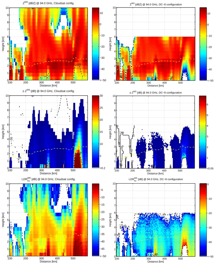
ized by the scattering properties of Fig. 3, is shown in the top panels of Fig. 4. The left panels correspond to a CloudSat configuration, the right panels to an airplane flying at 6 km altitude. In all the panels of Fig. 4 the dashed line repre-sents the contour level at –26/–40 dBZ for the SS reflectivity. When looking at the space-borne MS reflectivity (upper left panel) it is clear that, in SS configuration/regime, some of the regions close to the ground, due to attenuation problems, were below the MDT . However, they produce a detectable signal when MS signals are considered; in fact, MS maps the scattering from higher levels into these range bins, as de-tected by the radar. This is not true when considering the airborne configuration since in this case the SS and the MS contour levels are practically identical. The same conclusion can be made by looking at the central panels, that represent the MS enhancement (i.e. 1ZMS≡ZMS−ZSS) in the two configurations (note that in these panels undetectable regions below –26/–40 dBZ are blanked). While in the airborne con-figuration the MS enhancement is typically lower than 3 dB, there are regions in the spaceborne configuration, where the effect can reach extremely high values. To have a better dy-namic at low values the colorbar in the central left figure has been capped at 30 dB, but values as high as 79 dB are ac-tually reached in the region below the freezing level around 530 km. The radiation apparently sensed from those regions originates from waves scattered many times in the scatter-ing ice layer above. Theoretically the MS enhancement can be even infinite, e.g. for ranges longer than those associated with a finite-thick cloud: the signal we see from those ranges is actually produced completely in the upper levels and is to-tally independent of the clear sky response which would be expected in a SS regime.
This is better demonstrated in the two panels of Fig. 5. They correspond to two profiles extracted from the
Distance [km] Height [km] Hydrometeor profile [g/m3] 0.5 0.5 0.5 0.5 0.5 0.5 0.5 0.5 0.5 1 1 1 2 100 200 300 400 500 0 1 2 3 4 5 6 7 8 9 10 <0.01 0.5 1 1.5 2 Distance [km] Height [km] Extinction profile [km−1] @ 94.0 GHz 0. 5 0.5 0.5 0.5 0.5 0.5 2 2 4 100 200 300 400 500 0 1 2 3 4 5 6 7 8 9 10 <0.02 0.5 1 1.5 2 2.5 3 3.5 4 Distance [km] Height [km] Albedo profile @ 94.0 GHz 0. 2 0.2 0.2 0.2 0.2 0.2 0.2 0.2 0.2 0.2 0.2 0.2 0.2 0. 5 0.5 0.5 0.5 0.5 0.5 0.5 0.5 0.5 0.5 0.5 0.5 0.9 0.9 0.9 0.9 0.9 100 200 300 400 500 0 1 2 3 4 5 6 7 8 9 10 0.1 0.2 0.3 0.4 0.5 0.6 0.7 0.8 0.9 Distance [km] Height [km] g profile @ 94.0 GHz 0.2 0.2 0.2 0.2 0.2 0.2 0.2 0.2 0.2 0.2 0.2 0.5 0.5 0.5 0.5 0.5 0.5 0.5 0.5 0.5 0.5 0.5 0.5 0.5 0.8 100 200 300 400 500 0 1 2 3 4 5 6 7 8 9 10 0 0.1 0.2 0.3 0.4 0.5 0.6 0.7 0.8
Fig. 3. Cross section of a MidAtlantic Cold Front: hydrometeor content in g/m3(top left), extinction coefficient in km−1(top right), SS albedo (bottom left) and asymmetry parameter (bottom right) profiles. The yellow dash-dotted line corresponds to the freezing level altitude.
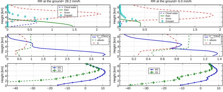
precipitating cell of the cold front at 536 km (left) and 548 km (right panels) with a rain rate at the ground equal respec-tively to 28.2 mm/h and 6.0 mm/h. This corresponds to a total optical thickness equal to 13.6 and 7.1 and to a scat-tering optical thickness equal to 7.8 and 4.8 respectively. Al-though quite different hydrometeor contents are present in the lower part of the two profiles, the MS reflectivity profiles look quite similar (continuous-crossed lines in the bottom panels of Fig. 5). In contrast the SS profiles (dashed-diamond lines) are quite different with the heavy precipitating profile (left panel) characterized by a strong decrease due to higher attenuation. The reason for this resides in both cases in the presence of a thick snow layer between about 8 and 2 km (top panel of Fig. 5) characterized by very high SS albedo (around 0.95) and high asymmetry parameter (around 0.8, center panel of Fig. 5). As a result, what the radar is sensing at an apparent altitude less than 2 km is not a signal coming from the rain layer in that altitude but it is the MS signature of the upper layer. Obviously the interpretation of a MS
sig-nal like the one shown in the lower panels of Fig. 5 in terms of SS approximation will lead to completely wrong conclu-sions.
Another remarkable feature in the central left panel of Fig. 4 is the strong MS effect present in the pixels close to the ground between 300 and 320 km. These pixels corre-spond practically to no hydrometeor content (see correcorre-spond- correspond-ing points in the top left panel of Fig. 3). The hydrometeor scattering properties and MS/SS reflectivity vertical pattern for a profile in this region (corresponding to drizzle evaporat-ing before hittevaporat-ing the ground) are shown in Fig. 6. The rain content reaches a maximum of 0.045 g/m3at 2 km (this cor-responds to a RR=0.5 mm/h for a Marshall and Palmer drop size distribution) but then decreases to 0 at the ground (see the continuous line in the top panel of Fig. 6). In this case the MS partially smoothens the transition at the cloud low-est boundary by spreading the cloud over a longer distance than its actual depth, an effect well known in the lidar com-munity (Bissonnette et al., 1995) and already indicated by the
Distance [km] Height [km] ZMS [dBZ] @ 94.0 GHz, Cloudsat config. −26 26 26 −26 100 200 300 400 500 0 1 2 3 4 5 6 7 8 9 10 <−50 −40 −30 −20 −10 0 10 Distance [km] Height [km] ZMS [dBZ] @ 94.0 GHz, DC−8 configuration −40 −40 −40 −40 −40 −40 −40 −40 −40 −40 −4 0 −4 0 −40 −40 −4 0 −40 −40 100 200 300 400 500 0 1 2 3 4 5 6 7 8 9 10 <−50 −40 −30 −20 −10 0 10 Distance [km] Height [km] ∆ Z MS [dB] @ 94.0 GHz, Cloudsat config. −26 −26 −26 −2 −26 100 200 300 400 500 0 1 2 3 4 5 6 7 8 9 10 <0.2 5 10 15 20 25 30 Distance [km] Height [km] ∆ Z MS [dB] @ 94.0 GHz, DC−8 configuration −40 −40 −40 −40 −40 −40 −40 −40 −40 −40 −40 −40−40 −4 0 −40 − 40 −40 100 200 300 400 500 0 1 2 3 4 5 6 7 8 9 10 <0.05 1 2 3 4 5 6 Distance [km] Height [km] LDRhvMS [dB] @ 94.0 GHz, Cloudsat config. −26 −26 26 −26 100 200 300 400 500 0 1 2 3 4 5 6 7 8 9 10 <−50 −45 −40 −35 −30 −25 −20 −15 −10 −5 Distance [km] Height [km] LDRhvMS [dB] @ 94.0 GHz, DC−8 configuration −40 −40 −40 −40 −40 −40 −40 −40 −40 −40 −40 −40 −40 −40 −40 100 200 300 400 500 0 1 2 3 4 5 6 7 8 9 10 <−50 −40 −30 −20 −10 0
Fig. 4. Radar quantities simulated in correspondence to the cross section of a MidAtlantic Cold Front depicted in Fig. 3. Top panels: MS
reflectivity; central panels: reflectivity enhancement due to MS; bottom panels: LDRhv. The panels on the left correspond to CloudSat
space-borne configuration (beamwidth 0.1◦, altitude 705 km) the panels on the right to DC-8 air-borne configuration (beamwidth 0.8◦,
0 0.5 1 1.5 2 0 2 4 6 8 Height [km] RR at the ground= 28.2 mm/h Cloud water Rain Snow Graupel 0 0.5 1 1.5 2 2.5 3 3.5 4 0 2 4 6 8 Height [km] k ext [1/km] albedo g −40 −30 −20 −10 0 10 0 2 4 6 8 Height [km] MS SS 0 0.5 1 1.5 2 0 2 4 6 8 Height [km] RR at the ground= 6.0 mm/h Cloud water Rain Snow Graupel 0 0.2 0.4 0.6 0.8 1 1.2 1.4 0 2 4 6 8 Height [km] k ext [1/km] albedo g −40 −30 −20 −10 0 10 0 2 4 6 8 Height [km] MS SS
Fig. 5. Heavy and medium rain case extracted from the Cold Front simulation. Top panels: hydrometeor content in g/m3. Central panels:
scattering properties. Bottom panels: ZMSand ZSSprofiles in dBZ for the space-borne configuration.
0 0.05 0.1 0.15 0.2 0.25 0.3 0.35 0.4 0.45 0 2 4 6 8 Height [km] RR at the ground= 0.0 mm/h Cloud water Rain Snow Graupel 0 0.1 0.2 0.3 0.4 0.5 0.6 0.7 0 2 4 6 8 Height [km] kext [1/km] albedo g −40 −30 −20 −10 0 10 0 2 4 6 8 Height [km] MS SS
Fig. 6. Profile with evaporating drizzle close to the ground extracted from the Cold Front simulation. Top panel: hydrometeor content in
g/m3. Central panel: scattering properties. Bottom panel: ZMSand
ZSSprofiles in dBZ for the space-borne configuration.
single-layer analyses performed in Sect. 5.3 of Battaglia et al. (2006a). This phenomenon has to be considered in the re-trieval algorithms for vertical cloud profiles especially when cloud boundaries are sought. The bottom panels of Fig. 4 represent the ratio between the cross and the copolar reflec-tivity signal, the LDRhv≡ZZhhhv (where the first/second pedex refers to the polarization state of the emitted/received radia-tion), for space-borne and airborne configurations. Note that this quantity is not measured by the actual configuration of
the Cloud Profiling Radar of CloudSat. In the space-borne configuration extraordinarily high values (up to –1.3 dB) can be noticed in some parts of the cross section. Since spherical particles are assumed in the study, these high LDRhvvalues can only be due to MS effects. With only spherical parti-cles assumed the first order of scattering cannot produce any cross-polarized signal. Since we have simulated the emis-sion of an h−polarized wave from the radar, the SS return can only be h−polarized. The return echo after more than one scattering event will tend to become more and more un-polarized. The LDR sensitivity to MS effects is greater than the reflectivity enhancement sensitivity to MS effects; in the spaceborne configuration, it can assume quite large values (around –15 dB at horizontal distances around 330 km in the bottom left panel of Fig. 4) at altitudes around 5 km where practically no backscattering enhancement is apparent. This large sensitivity makes the effects of MS in the LDR sig-nal visible in the air-borne configuration as well (see bottom right panel). Figure 7 shows the reflectivity and LDR pro-files at x=512 km for all three radar configurations (shown in three different colors). The SS reflectivity profile (continu-ous black line) shows strong attenuation below 3.5 km. For the ER-2 configuration the MS reflectivity profile is practi-cally the same (no significant difference between the green diamonds and the continuous black line) while MS enhance-ment becomes increasingly important moving to DC-8 (blue diamonds) and CloudSat configuration (red diamonds). Note that the profile is entirely detectable in the two last configu-rations only. For the ER-2, in the region below 1.1 km, the signal does not reach the MDT (and in fact this region is blanked in the center right and bottom right panels of Fig. 4). The LDR profiles (with scale at the top of the panel) are
−400 −35 −30 −25 −20 −15 −10 −5 0 5 10 15 1 2 3 4 5 6 Reflectivity [dBZ] Height [km] ZSS ZMS[ER−2] ZMS[DC−8] ZMS[CloudSat] −400 −35 −30 −25 −20 −15 −10 −5 0 1 2 3 4 5 6 LDR [dB] Height [km] ER−2 DC−8 CloudSat
Fig. 7. SS (continuous black line) and MS (symbol lines) reflec-tivity (top panel) and LDR (bottom panel) profiles extracted from the Cold Front simulation at x = 512 km in CloudSat (red colour), ER-2 (blue) and DC-8 (green) configurations.
drawn in the undetectable regions as well. As before the MS effect is more evident in the CloudSat configuration (red cir-cles), which has LDRs higher than –10 dB for all the pixels below 3.5 km. LDR values higher than –10 dB are found for the DC-8 and the ER-2 configurations below 2.6 and 1.4 km respectively as well. Finally, notice that, due to the high op-tical thickness, the results in the lower part are typically af-fected by Monte Carlo noise (especially when the highest vertical resolutions are employed).
2.3 General analyses
Hundreds of profiles extracted from different Cloud Resolv-ing Models representResolv-ing a cold front, a warm front, a tropical squall line over the Ocean and a convective system over the Amazon have been analyzed. In the former section, the
re-0 10 20 30 40 50 60 0 10 20 30 40 50 60 70 80 ∆ Z [dB] One−way attenuation [dB]
Fig. 8. Scatterplot of one way attenuation versus MS enhancement. Different symbols correspond to different CRM (triangles for the squall line, diamonds for the LBA convection, crosses for the warm front, dots and circle for the Cold front), different colours to differ-ent radar configurations [red: CloudSat configuration, blue: ER-2
configuration (i.e. 0.8◦beamwidth and 20 km flight altitude), green:
DC-8 configuration (i.e. 0.8◦beamwidth and 6 km flight altitude).
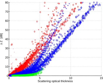
0 5 10 15 0 10 20 30 40 50 60 70 80 ∆ Z [dB]
Scattering optical thickness
Fig. 9. Scattering optical thickness versus MS enhancement. Dif-ferent symbols correspond to difDif-ferent CRMs, difDif-ferent colours to different radar configurations as described in caption of Fig. 8.
flectivity enhancement was often related to regions of high attenuation. This is more clearly illustrated in Fig. 8 where each point corresponds to one simulated bin with a reflectiv-ity above the MDT . Generally the MS enhancement 1ZMS increases with the one way attenuation (which is proportional to the optical distance travelled inside the medium). When using logarithmic units, the detected radar reflectivity at a
−250 −20 −15 −10 −5 0 5 10 15 20 25 30 35 40 45 50 LDRhvMS [dB] ∆ Z [dB]
Fig. 10. Scatterplots of LDR values versus MS reflectivity en-hancement for the space-borne (red colour), the stratosphere ER-2/DC-8 airborne configurations (blue and green colour). Different symbols correspond to different CRMs: diamonds for the LBA con-vection and dots for the Cold front.
range r can be written as:
ZMS[0 → r] = ZSS[0→r]+1ZMS[0→r]
=Ze[r]−A2−ways[0→r]+1ZMS[0→r] (1)
where all quantities but the effective reflectivity Ze are non local in the sense that they depend on the path between the radar (at range 0) and the bin (at range r). In Eq. (1)
1ZMScan be seen as a factor partially compensating for the two way attenuation. The plot in Fig. 8 has been clipped, i.e. some points with higher one way attenuation and 1ZMS do exist in the simulations (for some deep heavy precipitating profiles from the Amazon convective system). As demon-strated in the comparisons of the two panels of Fig. 5, in the presence of thick ice layers, the MS can become practically independent of the profile underneath so that it can enor-mously increase when highly attenuating media are present.
Note however also those few points with high 1ZMS at small attenuation. These points derive from cloud border ef-fects, as demonstrated when discussing Fig. 6. The different radar configurations (red for CloudSat, blue and green for airborne at 20 and 6 km altitude, respectively) lead to quite different reflectivity enhancements: while MS effects are ob-vious in the CloudSat configuration in regions of high atten-uation (red symbols) they are practically absent in the air-borne configuration at 6 km (1ZMS always less than 7 dB, green symbols). But they are still important when an air-borne stratospheric platform is deployed (blue symbols).
In Fig. 8 a strong dispersion is noted in the scatterplot: for the same attenuation a wide range of 1ZMSresults for each radar configuration. In particular, the presence of ice impacts the backscattering enhancement: with the same total optical
−25 −20 −15 −10 −5 0 5 10 0 5 10 15 20 25 30 35 40 Z [dBZ] ∆ Z MS [dBZ] 0.1 2 3.9 5.9 7.8 9.8
Fig. 11. Scatterplot of ZMSversus MS reflectivity enhancement in CloudSat configuration as a function of the rain rate at the ground (as readable in the colorbar). Different symbols correspond to dif-ferent CRM simulations.
thickness, profiles rich in ice particles will have more MS ef-fects. As demonstrated in Battaglia et al. (2006b) this can be better explained by using as reference variable the scatter-ing optical thickness, defined as the integral of the extinction coefficient weighted by the SS albedo over the vertical col-umn (Fig. 9). For a fixed scattering optical depth, there is now much less variability in 1ZMS. At high scattering op-tical depth a clear separation between the MidAtlantic front systems (dots and cross symbols) and the tropical systems (diamonds and triangles) is noticed. This relates to the dif-ferent microphysics prevalent in both mesoscale systems, in particular the different re-partitioning of the ice portion be-tween graupel and snow.
The discussion in Sect. 2.2 supports the idea that the LDR due to its high sensitivity can be used as an index for MS effects. This is demonstrated in Fig. 10 by including the results for all different configurations. For instance, LDR values lower than –10, –15 or –20 dB always guarantee that MS reflectivity enhancement will stay below 10, 5 or 1.5 dB respectively.
When considering low rain rate retrievals, it is important to assess whether or not MS effects have an impact on the derived rain rates profiles. Fig. 11 shows the reflectivity en-hancement for profiles with rain rates at the ground below 10 mm/h when the CloudSat configuration is considered. The colour scale is graduated according to the rain rate at the ground. The plot provides a rough idea about how much MS can affect rain rate retrievals. In particular it shows that the extension to rain rates higher than 1.5 mm/h needs to account for the presence of MS effects in the reflectivity signal. Even
0 0.2 0.4 0.6 0.8 1 0 2 4 6 8 Height [km] RR at the ground= 0.7 mm/h Rain Snow Graupel 0 0.2 0.4 0.6 0.8 1 0 2 4 6 8 Height [km] kext [1/km] albedo g −60 −4 −2 0 2 4 6 8 10 2 4 6 8 Height [km] MS SS
Fig. 12. Low rain case extracted from the Cold Front simulation.
Top panels: hydrometeor content in g/m3. Central panels:
scatter-ing properties. Bottom panels: ZMS and ZSSprofiles in dBZ for
the space-borne configuration.
for lower rain rates, the MS reflectivity profile may differ no-ticebly from the SS reflectivity profile in the lower part. As an example Fig. 12 shows the SS/MS reflectivity profiles for a rain rate at the ground equal to 0.7 mm/h: the SS re-flectivity is typically 4–5 dB lower than the MS rere-flectivity in the lower 3 km. Again we underline the fact that the MS effect is driven by the presence of a strongly forward scatter-ing ice layer. As a consequence similar considerations apply for snow-storm as well. Our results show that MS effects need to be accounted for when rainfall originating from mul-tiphase processes with rates higher than 0.5 mm/h or snowfall are considered.
3 Air-borne campaigns and validation of MS effects Air-borne campaigns have been carried out before the launch of the CloudSat mission. The Wyoming Cloud Radar (see Galloway et al. (1997) and references therein) has provided the first polarimetric airborne observations at 95 GHz. Ob-servations during field experiments in 1992 and 1994 show typical LDR features from the melting layer and from prefer-entially aligned ice crystals. During CRYSTAL-FACE (http: //cloud1.arc.nasa.gov/crystalface/) the Cloud Radar System (CRS, see Li et al. (2004)), operating at 94 GHz on board the NASA ER-2, acquired Doppler images over anvils generated by tropical maritime thunderstorms and over cirrus.
The data acquired by the Airborne Cloud Radar (ACR) sensor, mounted on a NASA P-3 aircraft, and flown over the Sea of Japan, the Western Pacific Ocean, and the Japanese Islands in the Wakasa Bay Field Campaign in January and
0 2 4 6 8 10 12 −70 −65 −60 −55 −50 −45 −40 −35 −30 −25 −20
Range from the radar [km]
MDT [dBZ]
Minimum detectable reflectivity
P t=1.4 kW Beamwidth=0.8 o Pulse length=0.8 µ s Noise figure=8.0 dB UTC [hour] Altitude [km]
Co−polar reflectivity date=20030123.094400
10.68 10.7 10.72 10.74 10.76 10.78 10.8 0 1 2 3 4 5 −30 −20 −10 0 10 20 30 surface echo UTC [hour] Altitude [km] LDR [dB] date=20030123.094400 10.68 10.7 10.72 10.74 10.76 10.78 10.8 0 1 2 3 4 5 −22 −20 −18 −16 −14 −12 −10 −8 −6 −4
Fig. 13. Top panel: minimum detectable reflectivity for the ACR system (relevant specifications are also listed). Detail of the copolar reflectivity (center panel) and the LDR (bottom panel) as measured by the ACR during the Wakasa Bay Experiment on the 23 January 2003.
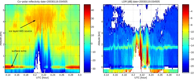
UTC [hour]
Altitude [km]
Co−polar reflectivity date=20030119.034505
4.14 4.16 4.18 4.2 4.22 4.24 4.26 4.28 4.3 0 1 2 3 4 5 −30 −20 −10 0 10 20 30 40 surface echo ice layer=MS source
UTC [hour] Altitude [km] LDR [dB] date=20030119.034505 4.14 4.16 4.18 4.2 4.22 4.24 4.26 4.28 4.3 0 1 2 3 4 5 −22 −20 −18 −16 −14 −12 −10 −8 −6 −4
Fig. 14. Detail of the copolar reflectivity and the LDR as measured by the ACR during the Wakasa Bay Experiment on the 19 January 2003.
February 2003 are found to be of particular interest for this study. This data set (plublicly available in netCDF via FTP, Stephens and Austin., 2004) includes 94 GHz co- and cross-polarized radar reflectivities. Flight legs were usually flown around 6400 m above mean sea level. The ACR has a beamwidth of 0.8◦and was usually operated with a vertical resolution of 120 m. The top panel of Fig. 13 shows the min-imum detectable reflectivity for the ACR system. Cross and co-polar reflectivities below this range-dependent threshold have been not considered in the analysis. Similarly LDR val-ues lower than –22 dB (a conservative estimate for the cross isolation term, see Wolde and Vali, 2001a) have been dis-charged.
In this database some interesting cases have been found with enhanced values of LDRs; examples are provided in Figs. 13–14. In both panels, the bright band can be seen as an horizontal strip with LDR values around –12 to –15 dB lo-cated at about 2.5 and 1.5 km. These bright band features are in agreement with former melting layer observations at ver-tical incidence during the Winter Icing and Storms Project (see Galloway et al., 1997). However much higher values of LDR (up to about –3 dB) are observed in coincidence in strongly attenuating regions (as indicated by the low surface echo in the reflectivity panels). These features do not seem to be produced by a low signal to noise ratio (a problem that was present in the dataset of the APR-2, see Im, 2003). In the analyses we have excluded all pixels with cross polar re-flectivity lower than –50 dBZ; they appear blank in Figs. 13– 14. By so doing we avoided the presence of possible high
LDR values at cloud boundaries (like in the upper right
cor-ner in Fig. 13). The remaining LDR features can hardly be explained from the SS point of view. Wolde and Vali (2001a,b) discuss polarimetric signatures as observed by the Wyoming airborne cloud radar at close distance which are
certainly not affected by propagation and MS effects. They report observations of high LDR with graupel in a cumu-lus congestus; however these values do not exceed –6 dB at side view and –9 dB when nadir looking (see their Fig. 6). Considering all incidence directions, the fuzzy logic algo-rithm described by Aydin and Singh (2004) assumes –5 dB as the highest possible value for LDR detectable from grau-pel particles (although non-spherical effects of melting par-ticles are still uncertain). The frequency of occurences of high LDR signatures in the Wakasa dataset is remarkable (while in Wolde and Vali (2001b) the frequency of occurence of LDR > −10 dB is very rare, especially at nadir view); if interpreted in terms of MS signal, the explanation seems straightforward and the observed patterns mirror those pro-duced by our simulations (like in Figs. 4–7). Note that the introduction of non-spherical particle scattering properties is not believed to change this LDR signature in a significative way just because this strong depolarization comes from the contribution of higher order of scattering.
4 Conclusions
The relevance of MS effects has been evaluated for the CloudSat configuration both for reflectivity enhancement and for the LDR signal (although such a quantity is not measured in the actual Cloud Profiling Radar of CloudSat). The sim-plified study conducted on a uniform layer reveals that large scattering optical thickness and asymmetry parameters are key factors in enhancing MS effects.
A typical midlatitude scenario has been analysed in detail to understand the relative importance of MS reflectivity en-hancement and LDR in vertically inhomogeneous profiles containing a mixture of hydrometeors. The intercomparison
between CloudSat and an airborne tropospheric airplane con-figuration reveals that the effect of the reflectivity enhance-ment is not detectable in the airborne configuration while it can be pretty large in regions of high attenuation for the spaceborne configuration. This is due to the much larger footprint of the space-borne system compared to the air-borne one as already discussed in Battaglia et al. (2005); Kobayashi et al. (2005). High LDR values are predicted for both configurations. These distinctive LDR signals are con-sistent with experimental data collected during the Wakasa Bay experiment, although non-spherical effects and instru-mental uncertainties have not been positively discounted.
The analysis of a wide range of profiles shows the strong correlation between the attenuation (and even more the scat-tering optical depth) and the MS reflectivity enhancement. Crucial to this correlation between attenuation and MS en-hancement is the role played by the the amount and the type of ice hydrometeors involved. Even for very low rain rates the presence of snow crystals or graupel particles aloft may induce MS reflectivity enhancements in the rain layer under-neath. This has to be taken into account when profiling algo-rithms are employed. In fact the MS effect can be interpreted as an effective reduction of the two-way attenuation by an amount equal to the MS enhancement. As a result rainfall estimates based on the SS approximation are believed to be burdened by positive biases.
If available with high cross-isolation, the measurement of the cross polarized signals can enormously help to detect areas potentially affected by MS enhancement since there is a clear relationship between this quantity and LDR val-ues. More studies on this topic are necessary to corrobo-rate our results, especially by exploiting air-borne polarized radar data derived in field campaigns. Due to the importance of SS scattering properties, a sensitivity study, including a better description of the ice segment of the cloud, will be conducted. When switching to non spherical ice particles the asymmetry parameter and the extinction coefficient – two key parameters affecting MS – generally are far apart from the equivolume sphere approximation counterparts (see Liu, 2004). The non spherical shape of raindrops is believed to play a minor role in modifying the SS properties. On the other hand, it will be obviously crucial for the correct compu-tation of the polarimetric variables. In particular, it is topic of future work the development of a polarized simulator which include non-spherical particles. This will provide a more comprehensive explanation of the still not well understood
LDR signatures detected by high frequency air-borne radars.
Acknowledgements. M. O. Ajewole is grateful to the Alexander von
Humboldt Foundation, the University of Bonn and the Federal Uni-versity of Technology of Akure for the research visit to Germany. The authors wish to thank all the Airborne Cloud Radar (ACR) team, which made available the dataset of 94 GHz co- and cross-polarized radar reflectivities collected during the Wakasa-Bay field experiment. (see http://nsidc.org/data/nsidc-0212.html).
Comments from the two reviewers were also very much appreci-ated.
Edited by: W. Conant
References
Aydin, K. and Singh, J.: Cloud Ice Crystal Classification Using a 95-GHz Polarimetric Radar, J. Atmos. Ocean Technol., 21, 1679–1688, 2004.
Battaglia, A., Ajewole, M. O., and Simmer, C.: Multiple scatter-ing effects due to hydrometeors on precipitation radar systems, Geophys. Res. Lett., 32, L19801, doi: 10.1029/2005GL023810, 2005.
Battaglia, A., Ajewole, M. O., and Simmer, C.: Evaluation of radar multiple scattering effects from a GPM perspective. Part I: model description and validation, J. Appl. Meteorol., 45, 1634–1647, 2006a.
Battaglia, A., Ajewole, M. O., and Simmer, C.: Evaluation of radar multiple scattering effects from a GPM perspective. Part II: model results, J. Appl. Meteorol., 45, 1648–1664, 2006b. Bissonnette, L. R., Bruscaglioni, P., Ismaelli, A., Zaccanti, G.,
Cohen, A., Benayahu, Y., Kleiman, M., Egert, S., Flesia, C., Schwendimann, P., Starkov, A. V., Noormohammadian, M., Op-pel, U. G., Winker, D. M., Zege, E. P., Katsev, I. L., and Polonski, I. N.: Lidar multiple scattering from clouds, Appl. Phys. B, 60, 355–362, 1995.
Bohren, C. F. and Huffman, D. R.: Absorption and Scattering of Light by Small Particles, John Wiley & Sons, New York, 1983. Galloway, J., Pazmany, A., Mead, J., McIntosh, R. E., Leon, D.,
French, J., Kelly, R., and Vali, G.: Detection of Ice Hydrome-teor Alignment Using an Airborne W-band Polarimetric Radar, J. Atmos. Ocean Technol., 14, 3–12, 1997.
Im, E.: APR-2 Dual-Frequency Airborne Radar Observations, Wakasa Bay, Japan, boulder, CO: National Snow and Ice Data Center. Digital media, 2003.
Kobayashi, S., Tanelli, S., and Im, E.: Second-order multiple-scattering theory associated with backmultiple-scattering enhancement for a millimeter wavelength weather radar with a finite beam width, Radio Sci., 40, RS6015, doi:10.1029/2004RS003219, 2005. L’Ecuyer, T. S. and Stephens, G. L.: An Estimation-Based
Precipi-tation Retrieval Algorithm for Attenuating Radars, J. Appl. Me-teorol., 41, 272–285, 2002.
Lhermitte, R.: A 94 GHz Doppler Radar for Cloud Observation, J. Atmos. Ocean Technol., 4, 36–48, 1987.
Lhermitte, R.: Attenuation and Scattering of Millimeter Wavelength Radiation by Clouds and Precipitation, J. Atmos. Ocean Tech-nol., 7, 464–479, 1990.
Li, L., Heymsfield, G. M., Racette, P. E., Tian, L., and Zenker, E.: A 94-GHz Cloud Radar System on a NASA High-Altitude ER-2 Aircraft, J. Atmos. Ocean Technol., 21, 1378–1388, 2004. Liu, Q.: Approximation of Single Scattering Properties of Ice and
Snow Particles for High Microwave Frequencies, J. Atmos. Sci., 61, 2441–2456, 2004.
Marzano, F. S., Roberti, L., Di Michele, S., Mugnai, A., and Tassa, A.: Modeling of apparent radar reflectivity due to convec-tive clouds at attenuating wavelenghts, Radio Sci., 38(1), 1002, doi:10.1029/2002RS002613, 2003.
Sadowy, G. A., McIntosh, R. E., Dinardo, S. J., Durden, S. L., Edel-stein, W. N., Li, F. K., Tanner, A. B., Wilson, W. J., Schnei-der, T. L., and Stephens, G. L.: The NASA DC-8 airborne cloud radar: design and preliminary results, in: Proceedings of IGARSS ’97, 4, 1466–1469, 1997.
Stephens, G. L.: Cloud Feedbacks in the Climate System: A Critical Review, J. Climate, 18, 237–273, 2005.
Stephens, G. L. and Austin., R. T.: Airborne Cloud Radar (ACR) Reflectivity, Wakasa Bay, Japan, boulder, CO: National Snow and Ice Data Center. Digital media, 2004.
Stephens, G. L., Vane, D. G., Boain, R. J., Mace, G. G., Sassen, K., Wang, Z., Illingworth, A. J., O’Connor, E. J., Rossow, W. B., Durden, S. L., Miller, S. D., Austin, R. T., Benedetti, A., Mitrescu, C., and Team, T. C. S.: The CLOUDSAT mission and the A-train, Bull. Am. Meteorol. Soc., 83, 1771–1790, 2002. Wolde, M. and Vali, G.: Polarimetric Signatures from Ice Crystals
Observed at 95 GHz in Winter Clouds. Part I: Dependence on Crystal Form, J. Atmos. Sci., 58, 828–841, 2001a.
Wolde, M. and Vali, G.: Polarimetric Signatures from Ice Crystals Observed at 95 GHz in Winter Clouds. Part II: Frequencies of Occurrence, J. Atmos. Sci., 58, 842–849, 2001b.