Preindustrial-to-present-day radiative forcing by tropospheric ozone from improved simulations with the GISS chemistry-climate GCM

(1)

HAL Id: hal-00301195

https://hal.archives-ouvertes.fr/hal-00301195

Submitted on 28 Jul 2003

HAL is a multi-disciplinary open access

archive for the deposit and dissemination of sci-entific research documents, whether they are pub-lished or not. The documents may come from teaching and research institutions in France or abroad, or from public or private research centers.

L’archive ouverte pluridisciplinaire HAL, est destinée au dépôt et à la diffusion de documents scientifiques de niveau recherche, publiés ou non, émanant des établissements d’enseignement et de recherche français ou étrangers, des laboratoires publics ou privés.

Preindustrial-to-present-day radiative forcing by

tropospheric ozone from improved simulations with the

GISS chemistry-climate GCM

D. T. Shindell, G. Faluvegi, N. Bell

To cite this version:

D. T. Shindell, G. Faluvegi, N. Bell. Preindustrial-to-present-day radiative forcing by tropospheric ozone from improved simulations with the GISS chemistry-climate GCM. Atmospheric Chemistry and Physics Discussions, European Geosciences Union, 2003, 3 (4), pp.3939-3989. �hal-00301195�

(2)

ACPD

3, 3939–3989, 2003 Preindustrial-to-present-day radiative forcing by tropospheric ozone D. T. Shindell et al. Title Page Abstract Introduction Conclusions References Tables Figures J I J I Back Close

Full Screen / Esc

Print Version Interactive Discussion

Atmos. Chem. Phys. Discuss., 3, 3939–3989, 2003 www.atmos-chem-phys.org/acpd/3/3939/

Atmospheric Chemistry and Physics Discussions

Preindustrial-to-present-day radiative

forcing by tropospheric ozone from

improved simulations with the GISS

chemistry-climate GCM

D. T. Shindell, G. Faluvegi, and N. Bell

NASA Goddard Institute for Space Studies, and Center for Climate Systems Research, Columbia University, New York, New York, USA

Received: 22 May 2003 – Accepted: 4 July 2003 – Published: 28 July 2003 Correspondence to: D. T. Shindell (dshindell@giss.nasa.gov)

(3)

ACPD

Full Screen / Esc

Abstract

The tropospheric chemistry model used at the Goddard Institute for Space Studies (GISS) within the GISS general circulation model (GCM) to study interactions between chemistry and climate change has been expanded and integrated into a version of the GCM with higher vertical resolution. The chemistry now includes peroxyacetyl-5

nitrates and non-methane hydrocarbons in addition to background NO_x-HO_x-O_x -CO-CH₄ chemistry. The GCM has improved resolution and physics in the boundary layer, improved resolution near the tropopause, and contains a full representation of the stratosphere. Simulations of present-day conditions show that this coupled chemistry-climate model is better able to reproduce observed tropospheric ozone, especially in 10

the tropopause region, which is critical to climate forcing. Comparison with simulations of preindustrial conditions gives a global annual average radiative forcing due to tro-pospheric ozone increases of 0.30 W/m2 with standard assumptions for preindustrial emissions. Locally, the forcing reaches more than 0.8 W/m2 in parts of the northern subtropics during spring and summer, and is more than 0.6 W/m2 through nearly all 15

the Northern subtropics and mid-latitudes during summer. An alternative preindustrial simulation with soil NO_x emissions reduced by two- thirds and emissions of isoprene, paraffins and alkenes from vegetation increased by 50% gives a forcing of 0.33 W/m2. Given the large uncertainties in preindustrial ozone amounts, the true value may lie well outside this range.

20

1. Introduction

Changes in atmospheric chemistry since the industrial revolution have had a significant impact on climate and human health, but are difficult to quantify accurately due to their complexity [Intergovernmental Panel on Climate Change (hereafter IPCC), 2001]. Increased anthropogenic emissions of greenhouse gases and ozone precursor gases 25

(4)

ACPD

Full Screen / Esc

and also alter the oxidation capacity of the troposphere. The latter change affects the lifetime of many trace gases, including methane, another powerful greenhouse gas. Tropospheric ozone changes have a spatial pattern that is extremely inhomogeneous, leading to similar inhomogenaity in its radiative forcing. We therefore feel it is useful to explore these chemical changes in a model in which they can be directly coupled to 5

the concurrent climate changes during the past and those projected for the future. The magnitude of the radiative forcing due to tropospheric ozone increases is rel-atively uncertain. This uncertainty arises from the paucity of observations during the preindustrial period, and the poor quality of those that do exist. Estimates are therefore based on model simulations, though these are subject to large uncertainties in emis-10

sions of ozone precursors in both modern and especially in preindustrial times. Though the IPCC presents estimates of the forcing from tropospheric ozone since the preindus-trial of+0.35 ± 0.15 W/m2, several recent studies have indicated that the value may actually be significantly larger. These studies are based upon preindustrial emissions of precursors adjusted within their uncertainties to give a better match to the purported 15

19th century observations of surface ozone (Mickley et al., 2001), or estimates con-strained by 20th century observations prior to the late 1970s onset of large amounts of stratospheric ozone depletion by chlorofluorocarbons (Shindell and Faluvegi, 2002). Both studies find that forcings of around 0.7 W/m2are reasonable.

Radiative forcing from tropospheric ozone is especially large (per unit ozone change) 20

near the tropopause (Hansen et al., 1997). Estimates of ozone change in this region are therefore especially important for evaluating ozone’s forcing. Ozone in this region is extremely sensitive to stratosphere-troposphere exchange and to production of NO_x by lightning (Grewe et al., 2001). Both these factors are only weakly constrained by present-day observations, and are largely unconstrained for the preindustrial era. It 25

is therefore a priority that the chemistry-climate models used to estimate tropospheric ozone’s radiative forcing provide accurate simulations in this region.

We have previously developed and evaluated a simplified tropospheric chemistry package within the GISS GCM and used that model to explore the preindustrial to

(5)

ACPD

Full Screen / Esc

present-day radiative forcing from tropospheric ozone (Shindell et al., 2001). That model has also been applied to study the relative importance of individual emission changes and climate responses since the preindustrial (Grenfell et al., 2001), for the future (Grenfell et al., 2003), to an investigation of the origin and variability of up-per tropospheric nitrogen oxides and ozone (Grewe et al., 2001), and to a study of 5

dynamical-chemical coupling across the tropopause (Grewe et al., 2002). Compari-son with observations for that model showed that it was able to simulate tropospheric ozone and related species reasonably well. However, with only 9 vertical layers, that model had very coarse resolution in the vicinity of the tropopause and a poor represen-tation of the stratosphere, so that its primary deficiency was in simulating stratosphere-10

troposphere exchange and tropopause region ozone accurately. We present here a new version of the GISS coupled chemistry-climate model with greater vertical reso-lution and a full representation of the stratosphere. Given the resulting large increase in the computational expense of the climate model portion of the simulation, it was rel-atively inexpensive to add to the chemistry. We have therefore expanded the original 15

simple HO_x-NO_x-O_x-CO-CH₄chemistry to include isoprene and the peroxyacetylnitrate (PAN), alkene, alkyl nitrate, paraffin and aldehyde families. This new model has been used to simulate present-day conditions, and has been extensively compared with ob-servations. We have then performed preindustrial simulations, and investigated the resulting radiative forcing.

20

2. Model description

2.1. Chemistry

The model includes the basic HO_x-NO_x-O_x-CO-CH₄ chemistry (HO_x = OH + HO2; NO_x= NO + NO2+ NO3+ HONO; Ox= O + O(1D)+ O3) described in Shindell et al. (2001), as well as the additional molecules and chemical reactions shown in Tables 1 25

(6)

ACPD

Full Screen / Esc

family members are assumed to be rapid enough to maintain steady-state (at night, however, NO_x changes are explicitly calculated). This allows a larger chemical time step and transport of the entire family as a single tracer. We also use “lumped fami-lies” for hydrocarbons and PANs, which is necessary for the model to run sufficiently rapidly to be useful for climate studies. Chemical reactions involving these gases are 5

based on the similarity between the molecular bond structures within each family using the reduced chemical mechanism called the Carbon Bond Mechanism 4 (Gery et al., 1989; Houweling et al., 1998). This scheme has been validated extensively against smog chamber experiments and more detailed chemical schemes (Gery et al., 1988; Derwent, 1990; Paulson and Seinfeld, 1992; Tonnesen and Jeffries, 1994). Standard 10

gas phase chemical reaction rates have been updated to recent values (Sander et al., 2000).

The chemical family approach of grouping radical species together, along with com-bining hydrocarbons with similar characteristics into lumped families, permits calcula-tions requiring the transport of only sixteen species in the GCM (Table 1). After combin-15

ing the short-lived radicals into equilibrated families, we find that all the species have long enough lifetimes that we can use an extremely simple explicit scheme to calculate chemical changes (except for HO_x, CH₃O₂, and C₂O₃, whose very short lifetimes keep them in equilibrium at all times). Calculations are performed using a chemical time step of 1 h.

20

The chemical scheme includes 77 reactions, 25 of which have been added to the previous scheme to account for reactions of PANs and NMHCs (Table 2). As with the simpler scheme, heterogeneous hydrolysis of N₂O₅ into HNO₃ takes place on sulfate aerosols, using the reaction rate coefficients given by Dentener and Crutzen (1993). Sulfate surface areas are taken from an online calculation performed with the 9-layer 25

version of the GISS GCM (Koch et al., 1999), assuming a monodispersed size dis-tribution. Photolysis rates are calculated every two hours using the Fast-J scheme (Wild et al., 2000). Phase transformations of soluble species are calculated based on the GCM’s internal cloud scheme. We include transport within convective plumes,

(7)

ACPD

Full Screen / Esc

scavenging within and below updrafts, rainout within both convective and large-scale clouds, washout below precipitating regions, evaporation of falling precipitation, and both detrainment and evaporation from convective plumes (Koch et al., 1999; Shindell et al., 2001). Dry deposition is based on a resistance-in-series calculation and pre-scribed (i.e. uncoupled) vegetation as depre-scribed in Shindell et al. (2001). Chemical 5

calculations are performed only in the troposphere in this version of the model, while stratospheric values of ozone, nitrogen oxides, and methane are prescribed according to satellite observations with seasonally varying abundances as in the standard GISS model (Hansen et al., 1996).

The model also includes a full representation of the global methane cycle, including 10

the chemical oxidation chain and detailed emissions and sinks. Though not crucial for the simulations described here, calculation of methane as an active chemical con-stituent will allow for future investigations of interactions between climate change and methane emissions and oxidation. Note that water vapor is also an active chemical tracer in this model, in contrast to most chemical models which lack a detailed hydro-15

logical cycle, and can thus respond to changes in climate via surface temperatures and altered circulation patterns.

2.2. Sources and sinks

Emissions of NO_x and CO are largely unchanged from our previous model, based largely on the Global Emissions Inventory Activity (GEIA) data sets (Benkovitz et al., 20

1996; Olivier et al., 1996) and on Wang et al. (1998a). Total emissions of CO are 987.7 Tg/yr (490.1 from biomass burning and 497.6 from industrial activities). Prescribed emissions of NO_xwere 20.9 Tg/yr N from fossil fuels, 5.8 from soils, 5.8 from biomass burning, and 0.6 from aircraft. We have added emissions of isoprene based on Wang et al. (1998a), and alkenes and paraffins also based on GEIA. Global annual average 25

emissions of isoprene were scaled to 200 Tg/yr from vegetation, as in recent model intercomparisons (IPCC, 2001). Global annual average emissions of alkenes are 32.9 Tg/yr, made up of 16.0 Tg/yr from vegetation, 11.6 Tg/yr from industry, and 5.3 Tg/yr

(8)

ACPD

Full Screen / Esc

from biomass burning. The largest single contributor is propene, which makes up nearly half the emissions for this family, with other alkenes and alkynes also contribut-ing. Global annual average emissions of paraffins are 87.0 Tg/yr, made up of 14.0 Tg/yr from vegetation, 68.8 Tg/yr from industry, and 4.2 Tg/yr from biomass burning. For the industrial component, butane, pentane and higher alkanes are the largest sources, 5

with smaller contributions from ethane and propane. The biomass burning component is dominated by ethane emissions. For both the alkene and paraffin families, the spatial and temporal distribution of isoprene emissions was used for vegetation, and that of carbon monoxide for biomass burning, for lack of further information, with the overall source value scaled to the emissions given above. Distributions of industrial emissions 10

of alkenes and paraffins are from GEIA.

Methane emissions were based upon the data sets of Fung et al. (1991) (available

athttp://www.giss.nasa.gov/data/ch4fung). These fields were scaled to values within

recent estimates of individual source strengths and their uncertainties (World Meteoro-logical Organization (hereafter WMO), 1999), but maintaining the spatial distributions 15

of the original data sets. The only exception was wetland emissions, which were shifted in latitude towards the tropics (x 1/3 poleward of 30◦ in both hemispheres, x 10/4 from 30◦S–30◦N) to match more recent estimates of their meridional distribution (WMO, 1995), and increased in magnitude to be more in line with recent estimates (Hein et al., 1997; Walter et al., 2001). Total emissions are 464.0 Tg/yr, made up of emissions 20

from the following individual sources (in Tg/yr): animals (enteric fermentation in rumi-nants plus animal waste) 83.9, coal mining 20.1, pipeline leakage of natural gas 24.8, venting of natural gas at wells 17.0, landfills (including municipal solid waste) 27.5, ter-mites 20.0, coal burning 16.0, ocean (including 3.0 from hydrates) 13.0, fresh water 5.0, miscellaneous ground sources (volcanoes and hydrothermal vents) 7.0, biomass 25

burning 30.0, rice cultivation 30.0, wetlands and tundra 209.7. Loss of methane via absorption into soils is also included, with a value of −39.9 Tg/yr (Fung et al., 1991; WMO, 1994). Biomass burning, rice cultivation and wetlands/tundra include seasonal emission cycles.

(9)

ACPD

Full Screen / Esc

As in the older model, the GISS convection scheme is used to derive both the total lightning and the cloud-to-ground lightning frequencies interactively in each grid box and at each time step (Price et al., 1997). Then the generation of NO_xfrom lightning is used to derive the NO_x produced, including a C-shaped vertical distribution (Pickering et al., 1998).

5

2.3. Climate model

The climate model used here is a version of the GISS model II’ (two-prime) en-hanced over that used previously with updated planetary boundary layer and convec-tion schemes. Briefly, the GCM’s boundary layer employs a finite modified Ekman layer with parameterizations for drag and mixing coefficients based on similarity theory, 10

convection includes entraining and nonentraining plumes, mass fluxes proportional to convective instability, explicit downdrafts, and a cloud liquid water scheme, based on microphysical sources and sinks of cloud water, which carries both water and ice (Del Genio et al., 1996). The land surface parameterization calculates transpiration, in-filtration, soil water flow and runoff, all of which impact both water vapor and latent 15

heat release to the atmosphere. Chemical tracers, along with heat and moisture, are advected using a quadratic upstream scheme (Prather, 1986). Momentum advection uses a fourth-order scheme. The model’s interhemispheric exchange times are within 15–25% of observations. Within the GISS chemistry modeling group we have focused on improving those aspects of the circulation that we believed would be most cru-20

cial for correctly simulating stratosphere-troposphere exchange. The gravity-wave drag scheme in this model version has been tested extensively and is now able to reproduce observed wind and temperature climatologies much better than in previous versions. This has led to notably improved transport of ozone down from the stratosphere, for ex-ample, which was heavily biased towards high latitudes and had an incorrect seasonal 25

cycle in other model versions.

All simulations with the new chemistry have been performed using a version with 4 × 5◦ horizontal resolution and 23 vertical layers (Fig. 1). Note that the vertical

(10)

ACPD

Full Screen / Esc

resolution has been significantly improved in both the boundary layer and near the tropopause, both regions crucial to ozone simulations, in addition to adding layers in the stratosphere (Fig. 1). The bottom 11 layers of this model are terrain-following lev-els, while the top 12 are constant pressure surfaces. The model time-step is one hour for both the chemistry and physics. Ozone calculated by the chemical model 5

is coupled to the GCM’s radiation calculation, so that chemical changes are able to affect meteorology. Monthly mean sea-surface temperatures and sea ice cover are prescribed to 1990–1999 average values (N. A. Rayner et al., Globally complete anal-yses of SST, sea ice, and night marine air temperature, 1871–2000, manuscript in preparation, 2003; hereafter Rayner SST 2003) in these simulations for computational 10

savings. Therefore the climate is not fully responsive to the chemistry. The importance of such coupling will be investigated in future simulations. All results presented here are averages over the last five years of seven year simulations. The model reaches equilibrium within the first year, and the interannual variability is relatively small com-pared to features of interest, so that five years gives us adequate statistics for mean 15

values. The model has been run for present-day (1990) and for preindustrial (∼1850) conditions. Additionally, a run with the older chemistry package lacking PANs and hydrocarbons higher than methane has been performed with the 23-layer GCM. This helps isolate the influence of the increased vertical resolution from the effect of the more sophisticated chemistry.

20

The more comprehensive chemistry scheme adds only about 24% to the running time of the GCM, plus an additional ∼15% for the transport of the chemical tracers, for a total increase of only ∼40%. It is therefore computationally rapid enough that the GCM can be run with online chemistry for long-term climate simulations or for multiple runs to examine the sensitivity of the results to various changes. Though the fractional 25

time used for chemistry is less for the more complex chemistry in the 23-layer model than for the simplified chemistry in the 9-layer model (∼40% versus ∼55%), this is only because the physics takes much longer in the 23-layer version, where the calculations are both more sophisticated and done on more vertical levels. The absolute time taken

(11)

ACPD

Full Screen / Esc

by the more complex chemistry is roughly a factor of 3 greater than for the simplified chemistry, both due to the increase in the number of reactions and tracers and to the increase of nearly a factor of two in the number of vertical levels within the troposphere.

3. Evaluation of present-day simulation

3.1. Ozone 5

We have compared modeled annual cycles of ozone with the ozonesonde climatology of Logan (1999). Comparisons at stations representative of a wide range of latitudes are shown in Fig. 2. Results from the earlier 9-layer model with simplified chemistry are also shown (for these comparisons, we have interpolated between model levels to the exact pressure levels of the sonde data, leading to slight differences as compared 10

with the results shown for the older model in Shindell et al. (2001)). The new model clearly does a better job at matching the observations than the older model at the levels nearest the tropopause (125 and 200 hPa). This holds for both the tropics, where the ozone is primarily of tropospheric origin, and for middle and high latitudes, where for at least part of the year the air is primarily of stratospheric origin. At 200 hPa, a positive 15

bias in the tropics in the 9-layer model has been eliminated. Comparison of the results from the 23-layer simulations using simplified chemistry against those with the more advanced scheme show that the improvement in this region results primarily from an improved representation of tropical upwelling rather than from chemistry. The model has difficulty reproducing the spring maximum in ozone at 200 hPa at Northern middle 20

and high latitudes, though it does this fairly well in the Southern Hemisphere. This maximum is stratospheric air, and thus may indicate biases in the stratospheric ozone climatology. It should be noted, however, that the vertical gradient of ozone is extremely large at these altitudes, so that small differences in height can lead to ozone changes of hundreds of ppbv (this is true at 125 hPa as well). It may be that a near-perfect match 25

(12)

ACPD

Full Screen / Esc

this area. For those locations and seasons dominated by tropospheric air (i.e. with ozone values less than about 150 ppbv, such as Hohenpeissenberg during September and October and Lauder during January to April), the model does an excellent job of reproducing observed values. Results are fairly similar in the middle troposphere between the old and new models, though the positive bias at high latitudes is somewhat 5

worse in the new version. Fortunately, these locations are less important for radiative forcing. At the surface most locations show small improvements, while the comparison with Hohenpeissenberg measurements is greatly improved. We attribute this largely to improvements in the boundary layer scheme of the GCM, including the higher vertical resolution there which allow more realistic dry deposition. Similar improvements in 10

surface ozone values were seen at Pretoria and Sapporo (not shown).

We compare the ability of the two model versions to reproduce the observations over all the sites recommended for testing models by Logan et al. (1999) in Table 3. As noted, the quality of the new model’s ozone simulation has improved markedly in the vicinity of the tropopause and near the surface. Biases in the vicinity of the tropopause 15

are now very small. Though the 125 hPa level is often in the stratosphere, and thus merely reflects the climatology, improvements in the tropics, where this level is in the troposphere have reduced the bias there from 5% to 3% comparing the new model to the older version. At 200 hPa, the bias has been greatly reduced, from 23% to 12%. A similar level of improvement has been obtained at low levels, where biases have 20

dropped to 11% and 8% at 500 and 950 hPa, respectively, from 16 and 31% in the older model. Similar improvements are apparent when examining the average abso-lute differences. In the middle troposphere, however, the average absolute difference between the model and the observations has increased. Evaluation of the average bias reveals that this results largely from a consistent positive bias in this region, much of 25

which comes from the two high-latitude sites (Table 3). This likely results from deficien-cies in the GCM’s downward transport of stratospheric air at high latitudes, which also seems to affect the 500 hPa level at high latitudes. The positive bias at 300 hPa may also be related to the lightning NO_xproduction, which may be on the high side though

(13)

ACPD

Full Screen / Esc

it is well within current uncertainty (see below, and note that reduced lightning NO_x would worsen the negative bias at 200 hPa). Except for the 300 hPa level, however, the systematic bias averaged over all 16 sites is roughly 10% or less. The average abso-lute difference between the model and the measurements is well within the observed standard deviation at all levels.

5

In general, the model does a good job of reproducing both the magnitude and sea-sonality of tropospheric ozone. While comparison between the 23-layer runs with sim-plified and advanced chemistry shows few obvious areas of improvement in the ozone fields, we nevertheless believe that incorporation of the advanced chemistry allows better simulation of tropospheric ozone in remote regions (where little validation data 10

is available) and of ozone changes as a function of time, as well as doing a better job with other trace gases.

Surface ozone is shown in Fig. 3. Observations are well reproduced over most re-gions in this model. The model’s surface level ozone over the remote North Atlantic during January is slightly greater than observations, 35–45 ppbv as compared with 15

measurements showing values of 30–40 ppbv (Parrish et al., 1998). The observational data however include only 4 years of measurements from Sable Island (44◦N, 60◦W) and a single year from the Azores (39◦N, 28◦W), so should be treated with some cau-tion. The addition of PANs has increased the amount of ozone in remote regions of the Northern Hemisphere, accounting for the increase here relative to the older model. 20

In remote regions of the Southern Hemisphere, the model does an excellent job of re-producing the observed values. The model finds July values of 25–35 ppbv at Syowa station, a location where most models underpredict ozone (Shindell et al., 2001). Over the Southern Hemisphere continents, surface ozone has decreased significantly com-pared with the previous model version. For example, surface ozone over South Amer-25

ica has dropped from 30–45 ppbv in the previous version to only 5–2 ppbv in the current model. The very low values seen in the new model during summer, 5–15 ppbv over the Amazon basin and 10–20 over the Brazilian savannah, are in agreement with mea-surements taken during the ABLE-2A summer campaign which showed near-surface

(14)

ACPD

Full Screen / Esc

ozone values of about 8–16 ppbv over the Amazon and slightly larger values over the savannah (Kirchoff, 1988; Emmons et al., 2000). We attribute this change to the in-crease in hydrocarbons, which in regions with relatively low abundances of NO_x lead to ozone destruction. Values over the Southern Hemisphere oceans are quite similar in the two models, supporting a terrestrial influence.

5

The ozone budget in the new model is substantially altered from the previous ver-sion. However, we caution that this may not be a very useful indicator of the veracity of ozone simulations. As discussed in Shindell et al. (2001), models report widely dif-fering budget values, yet all profess to simulate observed ozone amounts reasonably well. Furthermore, in testing the gravity-wave drag parameterization in the GCM, we 10

discovered that changes in the stratosphere-troposphere exchange by a factor of two are largely compensated for by adjustment of the chemical and dry deposition terms to yield almost the same ozone fields in most areas. Another example comes from com-paring the 9-layer simulation with the simplified chemistry to the 23-layer model with the same chemistry. Going to the higher resolution model reduced the stratosphere-15

troposphere exchange by 364 Tg/yr. In compensation for the reduced influx, the net tropospheric chemical production increased by 378 Tg/yr, leading to a relatively small increase in the ozone burden. Similarly, comparing the simulations of the 23-layer GCM using the previous, simplified chemistry and the present more complex scheme showed that the addition of higher hydrocarbon families and PANs caused an increase 20

in the net chemical production of ozone of 201 Tg/yr. With a similar stratosphere-troposphere exchange in these two runs, the dry deposition increased by 191 Tg/yr, largely balancing the chemical changes and leading to an increase of only 18 Tg in the tropospheric ozone burden. Thus the system appears to be highly buffered, and changes to a given factor in ozone’s budget often have little net effect. In the new 25

model, the tropospheric ozone budget in terms of annual average fluxes (Tg/yr) is+417 stratosphere-troposphere exchange, −1466 dry deposition, and+1049 chemistry. The resulting ozone burden is 349 Tg. For comparison, the budget of the previous version was+750 stratosphere-troposphere exchange, – 1140 dry deposition, +389 chemistry,

(15)

ACPD

Full Screen / Esc

and an ozone burden of 262 Tg. The values for dry deposition and chemistry found here are quite large, at the high end or outside the range reported for other models. Yet the tropospheric ozone burden is in good agreement with the 236-364 Tg range re-ported by other models (Roelofs and Lelieveld, 1995; Levy et al., 1997; Roelofs et al., 1997; Houweling et al., 1998; Wang et al., 1998b; Hauglustaine et al., 1998; Mickley et 5

al., 1999; Stevenson et al., 2000; Lelieveld and Dentener, 2000).

The stratosphere-troposphere exchange was calculated using the flux across the 150 hPa surface for both the 9- and 23-layer models. Given the large gradients in the tropopause region, the precise value of the exchange is sensitive to the specific def-inition chosen. If instead we use the flux across the 250 or 75 hPa surfaces, we find 10

values of 539 or 383 Tg/yr, respectively, in the new model. If we sum the horizon-tal and vertical fluxes across a surface at 300 ˙hPa poleward of 30◦ and at 100 hPa in the tropics, we find a total net flux of 342 Tg/yr. Consistent with this range, the net chemistry term over the varyingly defined troposphere ranges from 1142 to 927 Tg/yr. The stratosphere-troposphere exchange term is the only one to have reasonably good 15

constraints on its global value, which has been given a 450 Tg/yr best estimate with a 200–870 Tg/yr range for the cross-tropopause flux from ozone-NO_y tracer correlations (Murphy and Fahey, 1994), a value of 450–590 Tg/yr at 100 hPa based on satellite observations (Gettelman et al., 1997) and 390 Tg/yr at 150 hPa (Mickley et al., 1999) based on fluxes estimated from meteorological data (Appenzeller et al., 1996). Our 20

comparable values are in the range of these estimates, and much better than that seen in our previous model.

If the dry deposition and chemistry were both very much too large, we might expect that although the budget would not be greatly affected since these terms oppose one another, there would be a systematic bias toward underprediction of ozone at low lev-25

els and overprediction elsewhere. The comparison with sondes (Fig. 2 and Table 2) does not support such a bias. In fact, the improvement in simulated surface ozone in polluted areas is largely attributable to the new planetary boundary layer scheme’s en-hancement of dry deposition. Based on the observational constraint of the lowest level

(16)

ACPD

Full Screen / Esc

sonde data it appears that the faster dry deposition is more reasonable. We therefore believe that the budget is not a very useful constraint, aside from the stratosphere-troposphere exchange term, and that the key test is that we have demonstrated that the model does a reasonably good job of simulating observed ozone values.

3.2. Carbon monoxide 5

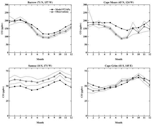
A comparison between observed and simulated annual cycles of surface carbon mox-ide at several locations is shown in Fig. 4. The model does a good job of matching the measured values, though there are slight positive and negative biases at Cape Mears and Samoa, respectively. Compared with the simpler chemistry, this version does a better job of reproducing the observed seasonal cycle, which matches the ob-10

servations quite well at all locations. The model has a global mean mass-weighted OH abundance of 9.7 × 105 molecules/cm3for the present day, matching the value of 9.4 ± 1.3 × 105molecules/cm3derived from measurements of the lifetime of the solvent methyl chloroform (Prinn et al., 2001). The ability of the model to reproduce the mean and seasonal cycle of CO so well implies that the seasonality and amount of hydroxyl 15

is well-simulated. Note that we have chosen to use a much reduced isoprene source in order to improve the carbon monoxide and hydroxyl simulations, despite the lack of observational support for such a source strength, as in recent intercomparisons (IPCC, 2001). If we use the emission source inferred from observations, we find the typical positive bias in CO and negative bias in OH. It remains to be determined whether 20

these biases result from deficiencies in current understanding of NMHC chemistry, in transport of emitted isoprene out of the canopy, or in some other factor.

3.3. Nitrogen species and lightning

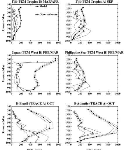
The budget of nitrogen oxides is shown in Table 4. We compare measurements of NO_x and HNO₃with modeled values in Fig. 5. Observations are not available with long-term 25

(17)

ACPD

Full Screen / Esc

with data obtained during brief field campaigns as compiled by Emmons et al. (2000). These may not be statistically representative, however. The sample of sites shown in the figure is representative of the behavior of many additional comparisons we per-formed. The model generally does a good job of reproducing observed profiles of NO_x. This is consistent with the model’s ability to accurately simulate ozone. The model 5

is generally capable of generating the very low values in the remote Pacific (Fig. 5). However, in a few regions, such as eastern Brazil (and southern Africa, not shown) the model cannot reproduce the very large values seen in the lower troposphere during the biomass burning period. Out over the South Atlantic the model gives a good match, but the continental values are too low, suggesting that at least during the year of the 10

TRACE-A observations, biomass burning emissions of NO_xmay have been larger than those in the GEIA inventory. Near highly polluted areas such as Japan, the model does an excellent job of matching the “C-shaped” profile found in observations (Fig. 5). In contrast to NO_x, the model’s simulation of HNO₃ is often not in accord with observa-tions in polluted regions. While the model mostly matches the observed profiles in the 15

remote Pacific and over the Philippine Sea, it greatly overpredicts nitric acid amounts over eastern Brazil, Japan, and the South Atlantic (Fig. 5), as well as over many other locations near biomass burning regions or industrialized areas (not shown). The over-prediction can be a factor of 5 or so, suggesting that the discrepancy is too large to be attributed simply to coarse model resolution or emission uncertainties. An over-20

predicition of nitric acid is a common problem in tropospheric chemistry models, and likely reflects a missing removal mechanism for nitric acid (since the NO_x values are reasonable). In the future, we intend to fully couple the chemistry in our model to the sulfate aerosol scheme, to consider the inclusion of ammonia chemistry, and to explore heterogeneous reactions on additional surface types such as mineral aerosols and ice 25

which may address this problem.

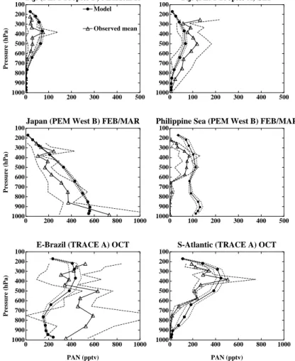
The model’s simulation of PANs is in fairly good agreement with observations in many locations (Fig. 6). PANs are underpredicted over Eastern Brazil during October, consistent with all the nitrogen species, and there is a suggestion of a systematic

(18)

ACPD

Full Screen / Esc

overestimate in polluted regions. As with nitric acid, we are hopeful that improvement of the model’s heterogeneous chemistry will address the latter problem. Additionally, our model uses a family of PANs, while the observations record only PAN itself, creating a systematic difference in the comparison.

The parameterized generation of NO_x from lightning produces 6.5 Tg/yr N in this 5

model. This is significantly larger than the previous model’s value of 3.9 Tg/yr, though within the expected range of 2–20 Tg/yr (WMO, 1999). The difference results from empirical adjustments made to the parameterization to better match observations, the altered convection scheme in the new model version, and the influence of the model’s higher vertical resolution on the lightning NO_xparameterization. The spatial distribution 10

of flashes is similar to that in the previous model, but is now in better agreement with Optical Transient Detector (OTD) satellite (Boccippio et al., 1998) observations (Fig. 7). The flash frequency averaged over all points is ∼25% greater in the GCM than in the observations, though there are underestimates over the oceans off the eastern edge of continents and over Northern Hemisphere middle latitudes. The older model produced 15

flash rates ∼60–65% of those observed. This suggests that the new parameterization and convection scheme likely gives a somewhat more realistic overall NO_x production from lightning, though the current production may be positively biased.

3.4. Hydrogen peroxide and methyl hydroperoxide

The model does a generally good job reproducing observed hydrogen peroxide values 20

in most regions regardless of season (Fig. 8). In contrast to the previous model version, the model is now able to capture the huge enhancement of H₂O₂ in the lower tropo-sphere over Brazil in the fall, albeit with a somewhat reduced magnitude (as expected from the NO_x bias). The model’s simulation over southern Africa during this time of year is also improved (not shown). The model exhibits a positive bias in the region of 25

900 hPa over portions of the Pacific similar to that shown for Fiji during March–April, but even larger at Tahiti, Hawaii, and Christmas Island. Given the overall high quality of the OH simulation, it seems likely that this is related to an underestimate of wet removal in

(19)

ACPD

Full Screen / Esc

this region. It is also possible that the model’s outflow of polluted air from Asia is too large, leading to too much chemical production of H₂O₂. Given the reasonably good quality of the simulated nitrogen oxides and nitric acid over the Pacific, however, this seems less likely.

The simulation of methyl hydroperoxide (CH₃OOH) is also quite good in this model 5

(Fig. 9). The model’s values are quite close to those observed for nearly all locations, including both highly polluted regions and the remote Pacific, and for all seasons. Ac-curate simulation of this important radical intermediate gives us confidence that the model’s chemical oxidation of hydrocarbons is being calculated reliably.

3.5. Methane 10

The methane oxidation rate is 431 Tg/yr, consistent with the budget of methane given its large uncertainties. The interhemispheric gradient of methane is ∼150 ppbv in these simulations (between averages over mid-to-high southern and northern latitude), in good agreement with 1990 observations (GLOBALVIEW-CH₄, 2001). This is not too surprising as the global OH values and the seasonal cycle of CO agree well with ob-15

servations, implying that the oxidation is well modeled. We note that the model has more OH in the Northern Hemisphere than in the Southern, as in most models, but in contrast to the estimates of Prinn et al. (2001) (though those estimates have a very large uncertainty). Were the chemistry to produce an OH distribution matching those results, however, the interhemispheric gradient would grow larger. The seasonal cycle 20

of methane appears exaggerated at high northern latitudes, however, though it is rea-sonable in the tropics and in the Southern Hemisphere. Future work will endeavor to improve the seasonality of our methane emissions datasets.

(20)

ACPD

Full Screen / Esc

4. Preindustrial to present-day change

Many factors related to chemistry and climate have changed since the industrial rev-olution. A systematic study of the effect of each individual change with our previous model demonstrated that the reduced emissions of nitrogen oxides and methane dom-inated the overall forcing of tropospheric ozone change (Grenfell et al., 2001). To 5

simulate preindustrial conditions, emissions of anthropogenic ozone precursors were eliminated (fossil fuels, industry and aircraft). Emissions from biomass burning were reduced to one-tenth of their present-day values, a common assumption also used in our earlier experiments. Sulfate surface areas were set to natural background lev-els as calculated by Koch et al. (1999). Monthly mean sea surface temperatures and 10

sea ice conditions were prescribed according to reconstructed values from the 1870s (Rayner SST 2003). The cooling relative to the present would be slightly larger for 1850 conditions, but this should have a minimal impact on the results (Grenfell et al., 2001). Concentrations of long-lived greenhouse gases were reduced as follows: CO₂ from 365 to 280 ppmv, N₂O from 314 to 275 ppbv, CH₄ from 1.745 to 0.700 ppmv, and 15

CFCs to zero. Production of NO_xby lightning decreased to 6.2 Tg/yr in the preindustrial simulations, exhibiting a sensitivity to climate change in line with the+10% per degree of surface warming for this parameterization (Price and Rind, 1994).

Tropospheric ozone levels have increased markedly since the preindustrial (Fig. 10). Abundances have roughly doubled over much of the Northern Hemisphere from the 20

equator to 45◦N, with increases of more then 100% at low altitudes. The total tropo-spheric ozone burden has gone from 255 Tg to 349 Tg. This represents an increase of 37%, in accord with the 25–57% range reported in other models (Levy et al., 1997; Roelofs et al., 1997; Mickley et al., 1999; Lelieveld and Dentener, 2000) and similar to the 45% increase seen in our earlier simulations (Shindell et al., 2001). The tropo-25

spheric ozone budget for the preindustrial simulations is+449 Tg/yr from stratosphere-troposphere exchange, −829 Tg/yr from dry deposition, and+380 Tg/yr from chem-istry. The strong dry deposition in this model draws down ozone so much that the net

(21)

ACPD

Full Screen / Esc

chemical term is positive, in contrast to the previous version. Given that the net term is the difference between two very large production and destruction terms, this change is in fact not as large as it might appear. As with the present day simulations, we caution that the budget values may not provide a very useful measure of the ozone simulation. Overall, the pattern of ozone increase is fairly similar to that seen in other models and 5

in our earlier simulations. However, the region of greatest increase (in ppbv) has shifted in comparison to our earlier simulations from about 80◦N between ∼600 and 80 hPa to 40◦N from ∼250 to 500 hPa. In percentage terms, the largest increase in both models takes place at Northern mid-latitudes near the surface. Increases of 80% now extend up to 250 hPa, while in the previous model version these went up to only ∼500 hPa. 10

The sensitivity above 500 hPa has likely been altered by the addition of non-methane hydrocarbons, which increased ozone production at upper levels, as seen in other models (e.g. Wang et al., 1998c). Enhanced lightning NO_xrelative to the older model may have also contributed to the different response. The stratosphere-troposphere ex-change was a greater contributor to tropospheric ozone in the preindustrial simulation 15

than for the present day; 449 Tg/yr as compared to 417 Tg/yr. Analysis of the ozone fluxes reveals that this was primarily a result of the decreased upward flux of ozone from the troposphere at low latitudes, rather than a sizeable change in the downward flux from the stratosphere. Since the improved vertical resolution allowed a better sim-ulation near the tropopause, and higher hydrocarbons are now included, the ozone 20

changes simulated with the current model should be more trustworthy, especially in the upper troposphere. Occurring near the tropopause, they will certainly affect the radiative forcing, which we discuss further below.

The oxidation capacity of the troposphere has also changed since the preindustrial (Fig. 11). Near the surface in the Northern Hemisphere, the large increase in pollution 25

in the present has caused a substantial increase in the abundance of OH, up to 50% in some locations. Hydroxyl production is increased by direct production via the O(1D) reaction with water, which is enhanced both by the global warming-induced increase in water vapor and the ozone pollution-induced increase in photolytic production of

(22)

ACPD

Full Screen / Esc

O(1D). Furthermore, the increased hydrocarbons lead to HO_x production, though they also reduce the amount of OH by conversion to HO₂. In regions with less abundant NO_x, such as the Southern Hemisphere and the middle and upper troposphere in the Northern Hemisphere, the latter effect dominates, so that the amount of OH has decreased in those areas despite the increased ozone and water vapor. In the heavily 5

polluted regions of the Northern Hemisphere, however, the hydrocarbon production of HO_x dominates, so that they further add to the overall increase in OH. The offsetting influences of the regions that show OH increases with those that show decreases leads to an overall OH reduction of 13.3% from the preindustrial to the present. Other models have reported responses ranging from 17% decreases to 6% increases (Brasseur et 10

al., 1998; Mickley et al., 1999; Berntsen et al., 1997). The reduction in OH calculated here yields a comparable increase in the lifetime of methane.

5. Radiative forcing

The global mean annual average radiative forcing at the tropopause from the tropo-spheric ozone increase between the preindustrial and the present-day is 0.30 W/m2in 15

these simulations (Fig. 12). The forcing is larger in the Northern Hemisphere, where its average value is 0.38 W/m2, than in the Southern Hemisphere where its average values is only 0.22 W/m2. Maximum forcings of 0.7 W/m2 occur in the Northern sub-tropics, where the ozone changes also maximized and where sunlight is plentiful. The forcing drops below 0.1 W/m2 only over Antarctica, where the ozone increases have 20

been smallest and insolation is weakest. The spatial pattern of the forcing in this model looks quite similar to the results of other groups as shown, for example, in the IPCC report (2001). Seasonally, the greatest forcing is during July-August (and is nearly as large during March–May), when the forcing is larger than 0.6 W/m2over nearly the en-tire Northern Hemisphere subtropics and mid-latitudes, and surpasses 0.8 W/m2over 25

parts of the subtropics (Fig. 13). The radiative forcing was calculated by calling the radiation code twice, once with the climatological ozone and once with the model’s

(23)

cal-ACPD

Full Screen / Esc

culated distribution. Then the change in this difference between the preindustrial and the present-day was calculated. Note that these results are not directly comparable to those presented for our previous model, which were for the top of the atmosphere rather than the tropopause. We believe the latter is a more useful diagnostic. The radia-tive forcing is primarily driven by absorption of longwave radiation (Fig. 14). Shortwave 5

radiation plays the dominant role only at high latitudes, where the albedo is very high. The global annual average forcing calculated here, 0.30 W/m2, is in accord with the range of 0.28 - 0.55 W/m2reported by other three-dimensional global models (Hauglus-taine et al., 1994; Roelofs et al., 1997; van Dorland et al., 1997; Berntsen et al., 1997; Stevenson et al., 1998; Haywood et al., 1998; Brasseur et al., 1998; Kiehl et al., 1999; 10

Mickley et al., 1999; Lelieveld and Dentener, 2000). The uncertainty associated with this forcing is quite large, however, as the preindustrial sources are poorly constrained. To explore the range of potential preindustrial ozone levels, we performed an additional preindustrial run setting the soil NO_xemissions, much of which result from fertilizer ap-plication, to one-third their present-day value and increasing the emission of isoprene, 15

paraffins and alkenes from vegetation by half to account for greater forested area in the past, following Mickley et al. (2001). In the “standard” preindustrial run, all of these emissions were kept unchanged from present-day values. The resulting global mean annual average radiative forcing from the present to the “alternative” preindustrial was 0.33 W/m2, with a spatial distribution very similar to that seen in the “standard” case 20

(Fig. 12).

A common test of preindustrial simulations is to compare with purported nineteenth century surface observations. We refer to these as “purported” observations due to their lack of quantitative reliability. Nearly all of these measurements were taken with a method known as the Sch ¨onbein technique, involving exposure of a chemically treated 25

piece of paper to the air. Modern evaluations of this technique have shown that the results are highly dependent upon a variety of factors, such as the exposure time or the type of paper used, which were not controlled in the early observations (Kley et al., 1988; Pavelin et al., 1999). These results are thus useful primarily in a

(24)

qualita-ACPD

Full Screen / Esc

tive sense. The only exceptions are the measurements from Montsouris, which were performed with a quantitative technique (Volz and Kley, 1988) (though even those data were affected by the influence of SO2and they may only reflect local conditions in the vicinity of Paris (Staehelin et al., 1994)). Though of limited quantitative use, we com-pare model results from the two preindustrial simulations with the nineteenth century 5

purported observations (Fig. 15). The “alternative” simulation appears to do a slightly better job of matching the data points. As with other models (e.g. Mickley et al., 2001), there is little evidence of a seasonal cycle at Luanda and a mild positive bias remains at Montsouris. In any case, there is certainly no evidence to suggest that the larger ozone changes and radiative forcing associated with the “alternative” preindustrial run 10

are too large.

6. Discussion and conclusions

We have developed an improved tropospheric chemistry model which has been cou-pled to a version of the GISS climate model with enhanced vertical resolution in the boundary layer, near the tropopause, and in the stratosphere. The new chem-15

istry scheme now includes both peroxyacetylnitrates and non-methane hydrocarbons. Through the use of chemical families and a simple explicit chemical solver, the model’s computational expense has been kept quite low. Nevertheless, the model does a rea-sonably good job of reproducing observed annual cycles and vertical profiles of ozone at many locations. The model’s main bias is an overestimation of ozone in the mid-20

dle troposphere at high-latitudes. This has a minimal effect on radiative forcing since insolation is weakest near the poles. The present model calculates a tropopause ra-diative forcing due to tropospheric ozone increases between the preindustrial and the present of 0.30 W/m2. Given the increased resolution near the tropopause, a region of paramount importance for radiative forcing, and the improved chemistry, we believe 25

the current results are more trustworthy than those of our earlier simulations.

(25)

how-ACPD

Full Screen / Esc

ever, primarily due to the extremely poor constraints on preindustrial emissions of ozone precursors. We performed a test of altered assumptions for preindustrial emis-sions for comparison with the results of another chemistry model used with a simpler version of the GISS GCM (Mickley et al., 2001). The results of Mickley et al. (1999) showed a radiative forcing of 0.44 W/m2 in their standard simulations. In our standard 5

preindustrial case, soil NO_x emissions were unchanged from the present, while in the Mickley et al. (1999) simulations, soil NO_x emissions from fertilizer were removed. An additional difference between the models is that Mickley et al. (1999) used a larger biomass burning NO_x source, making the reduction to preindustrial times (based on a 90% decrease) also larger. However, an additional run of our new model using 7.7 10

Tg/yr N from biomass burning (van Aardenne et al., 2001) compared with the standard preindustrial run gave an identical forcing to our initial present-day simulation (using 5.3 Tg/yr N from biomass burning), suggesting that the forcing is not greatly sensitive to these emissions. Overall then, the emission differences are consistent with the larger radiative forcing found in Mickley et al’s standard preindustrial to present-day case, 15

though differences in the GCM versions used likely also contributed. Using altered as-sumptions for preindustrial emissions of soil NO_x, hydrocarbons from vegetation, and lightning, Mickley et al. (2001) found a radiative forcing of 0.72–0.80 W/m2. They con-cluded that the increased forcing arose primarily from lightning, which they reduced by 43–71% (1.5-2.5 Tg N/yr). As our lightning change was only 5% (0.3 Tg N/yr), it is 20

not surprising that our alternative simulation of the preindustrial showed less of an in-crease in the forcing. Given current uncertainties in the sensitivity of lightning to climate change, it remains unknown how large the change in that source really has been. Our sensitivity of lightning to climate may be on the low side, however, as a recent study suggests a sensitivity (lightning flash rate increase per degree of surface warming) of 25

∼40%/K (Reeve and Toumi, 1999), as opposed to the ∼10%/K sensitivity in the Price and Rind (1994) parameterization used here. Additionally, our preindustrial simulation was driven by sea-surface temperatures from the 1870s (the earliest in the data set), which neglects a small portion of the warming since the preindustrial, thus giving the

(26)

ACPD

Full Screen / Esc

lightning less to respond to. Finally, these simulations did not account for any changes in stratospheric ozone, which could have affected both stratosphere-troposphere ex-change and the flux of OH-forming ultraviolet radiation reaching the troposphere.

In addition to using models to estimate the preindustrial to present-day radiative forc-ing due to tropospheric ozone, another study has examined the earliest available ozone 5

observations dating from the middle part of the twentieth century to evaluate long-term ozone trends (Shindell and Faluvegi, 2002). They concluded that the radiative forcing due to tropospheric ozone increases from the late 1950s to 2000 was 0.38± 0.10 W/m2. Assuming even a very modest ozone buildup prior to 1950, the forcing since the prein-dustrial would then have been in the area of 0.5–0.6 W/m2, on the high side of most 10

global model simulations. Extrapolating based on the rate of increase of NO_xemissions (van Aardenne et al., 2001), the ozone precursor which is most often rate limiting, the radiative forcing would have been about 0.6 W/m2(Shindell and Faluvegi, 2002). Thus the radiative forcing from tropospheric ozone remains poorly constrained from both ob-servations and models, but within the range of plausible values, it may have been one 15

of the most important greenhouse gas forcings of modern climate change.

Acknowledgements. The authors thank NASA’s Atmospheric Chemistry Modeling and

Analy-sis Program for support, the Global Hydrology Resource Center at the Global Hydrology and Climate Center for supplying the archived OTD data, J. Logan and L. K. Emmons for kindly providing observational data, and Y. Hu for extensive testing and improvements to the GCM’s

20

gravity-wave parameterization.

References

Appenzeller, C., Holton, J. R., and Rosenlof, K. H.: Seasonal variation of mass transport across the tropopause, J. Geophys. Res., 101, 15 071–15 078, 1996.

Benkovitz, C. M., Scholtz, M. T., Pacyna, J., Tarrason, L., Dignon, J., Voldner, E. C., Spiro, P.

25

A., Logan, J. A., and Graedel, T. E.: Global gridded inventories of anthropogenic emissions of sulfur and nitrogen, J. Geophys. Res., 101, 29 239–29 253, 1996.

(27)

ACPD

Full Screen / Esc

Berntsen, T. K., Isaksen, I. S., Myhre, G., Fuglestvedt, J. S., Stordal, R., Larsen, T. A., Freckle-ton, R. S., and Shine, K. P.: Effects of anthropogenic emissions on tropospheric ozone and its radiative forcing, J. Geophys. Res., 102, 28 101–28 126, 1997.

Boccippio, D. J., Driscoll, K., Koshak, W., Blakeslee, R., Boeck, W., Mach, D., Christian, H. J., and Goodman, S. J.: Cross-sensor validation of the Optical Transient Detector (OTD), J.

5

Atmos. Sol. Terr. Phys., 60, 701–712, 1998.

Brasseur, G. P., Kiehl, J. T., M ¨uller, J. F., Schneider, T., Granier, C., Tie, X., and Hauglustaine, D.: Past and future changes in global tropospheric ozone: Impact on radiative forcing, Geophys. Res. Lett., 25, 3807–3810, 1998.

Del Genio, A., Yao, M.-S., Kovari, W., and Lo, K. K.-W.: A prognostic cloud water

parameteriza-10

tion for global climate models, J. Clim., 9, 207–304, 1996.

Dentener, F. J. and Crutzen, P. J.: Reaction of N₂O₅on tropospheric aerosols: Impact on the global distributions of NO_x, O₃and OH, J. Geophys. Res., 98, 7149–7163, 1993.

Derwent, R. G.: Evaluation of a number of chemical mechanisms for their application in models describing the formation of photochemical ozone in Europe, Atmos. Env., 30, 2615–2624,

15

1990.

Emmons, L. K., Hauglustaine, D. A., M ¨uller, J. F., Carroll, M. A., Brasseur, G. P., Brunner, D., Staehelin, J., Thouret, V., and Marenco, A.: Data composites of airborne observations of tropospheric ozone and its precursors, J. Geophys. Res., 105, 20 497–20 538, 2000. Fung, I., John, J., Lerner, J., Matthews, E., Prather, M., Steele, L.P., and Fraser, P.J.:

Three-20

dimensional model synthesis of the global methane cycle, J. Geophys. Res. 96, 13 033– 13 065, 1991.

Gery, M. W., Whitten, G. Z., Killus, J. P., and Dodge, M. C.: Development and testing of the CBM-4 for urban and regional modelling, Rep. EPA-600/3-88-012, U. S. Environ. Prot. Agency, Research Triangle Park, NC, 1988.

25

Gery, M. W., Whitten, G. Z., Killus, J. P., and Dodge, M. C.: A photochemical kinetics mecha-nism for urban and regional scale computer modeling, J. Geophys. Res., 94, 925–956, 1989. Gettelman, A., Holton, J. R., and Rosenlof, K. H.: Mass fluxes of O₃, CH₄, N₂O, and CF₂Cl₂in the lower stratosphere calculated from observational data, J. Geophys. Res., 102, 19 149– 19 159, 1997.

30

GLOBALVIEW-CH 4: Cooperative Atmospheric Data Integration Project – Methane. CD-ROM, NOAA CMDL, Boulder, Colorado [Also available on Internet via anonymous FTP to ftp.cmdl.noaa.gov, Path: ccg/ch4/GLOBALVIEW], 2001.

(28)

ACPD

Full Screen / Esc

Grenfell, J. L., Shindell, D. T., Koch, D., and Rind, D.: Chemistry-climate interactions in the Goddard Institute for Space Studies general circulation model 2. New insights into modeling the preindustrial atmosphere, J. Geophys. Res., 106, 33 435–33 452, 2001.

Grenfell, J. L., Shindell, D. T., and Grewe, V.: Sensitivity studies of oxidative changes in the troposphere in 2100 using the GISS GCM, Atmos. Chem. Phys. Disc., 3, 1805–1842, 2003.

5

Grewe, V., Brunner, D., Dameris, M., Grenfell, J. L., Hein, R., Shindell, D., and Staehelin, J.: Origin and variability of upper tropospheric nitrogen oxides at northern midlatitudes, Atmos. Env., 35, 3421–3433, 2001.

Grewe, V., Reithmeier, C., and Shindell, D. T.: Dynamical-chemical coupling of the upper tropo-sphere and lower stratotropo-sphere region, Chemotropo-sphere, 47, 851–861, 2002.

10

Hansen, J., Sato, M., Ruedy, R., et al.: A Pinatubo climate investigation, in The Effects of Mt. Pinatubo Eruption on the Atmosphere and Climate, NATO ASI Ser. Subser. 1, Global Environment Change, edited by G. Fiocco, D. Fua, and G. Visconti, 233–272, Springer-Verlag, New York, 1996.

Hansen, J., Sato, M., and Ruedy, R.: Radiative forcing and climate response, J. Geophys. Res.,

15

102, 6831–6864, 1997.

Hauglustaine, D. A., Granier, C., Brasseur, G. P., and Megie, G.: The importance of atmospheric chemistry in the calculation of radiative forcing on the climate system, J. Geophys. Res., 99, 1173–1186, 1994.

Hauglustaine, D. A., Brasseur, G. P., Walters, S., Rasch, P. J., M ¨uller, J. F., Emmons, L. K., and

20

Carroll, M. A.: MOZART: A global chemical transport model for ozone and related chemical tracers, 2, Model results and evaluation, J. Geophys. Res., 103, 28 291–28 335, 1998. Haywood, J. M., Schwarzkopf, M. D., and Ramaswamy, V.: Estimates of radiative forcing due

to modeled increases in tropospheric ozone, J. Geophys. Res., 103, 16 999–17 007, 1998. Hein, R., Crutzen, P. J., and Heimann, M.: An inverse modeling approach to investigate the

25

global atmospheric methane cycle, Global Biogeochem. Cycles, 11, 43–76, 1997.

Houweling, S., Dentener, F., and Lelieveld, J.: The impact of non-methane hydrocarbon com-pounds on tropospheric photochemistry, J. Geophys. Res., 103, 10 673–10 696, 1998. Intergovernmental Panel on Climate Change, Climate Change 2001. J. T. Houghton, et

al. (eds). Cambridge University Press, Cambridge, England, 881 pp, 2001.

30

Kiehl, J. T., Schneider, T. L., Portmann, R. W., and Solomon, S.: Climate forcing due to tropo-spheric and stratotropo-spheric ozone, J. Geophys. Res., 104, 31 239–31 254, 1999.

(29)

ACPD

Full Screen / Esc

1476, 1988.

Kley, D., Volz, A., and Mulheims, F.: Ozone measurements in historic perspective, in Tropo-spheric Ozone, I. S. A. Isaksen (Ed.), D. Reidel Publishing Co., 63–78, 1988.

Koch, D., Jacob, D., Tegen, I., Rind, D., and Chin, M.: Tropospheric sulfur simulation and sulfate direct radiative forcing in the Goddard Institute for Space Studies general circulation model,

5

J. Geophys. Res., 104, 23 799–23 822, 1999.

Lelieveld, J. and Dentener, F. J.: What controls tropospheric ozone?, J. Geophys. Res., 105, 3531–3551, 2000.

Levy, H. II, Kasibhatla, P. S., Moxim, W. J., Klonecki, A. A., Hirsch, A. I., Oltmans, S. J., and Chameides, W. L.: The global impact of human activity on tropospheric ozone, Geophys.

10

Res. Lett., 24, 791–794, 1997.

Logan, J. A., An analysis of ozonesonde data for the troposphere: Recommendations for testing 3-D models and development of a gridded climatology for tropospheric ozone, J. Geophys. Res., 104, 16 115–16 149, 1999.

Mickley, L. J., Murti, P. P., Jacob, D. J., Logan, J. A., Koch, D. M., and Rind, D.: Radiative forcing

15

from tropospheric ozone calculated with a unified chemistry climate model, J. Geophys. Res., 104, 30 153–30 172, 1999.

Mickley, L. J., Jacob, D. J., and Rind, D.: Uncertainty in preindustrial abundance of tropospheric ozone: Implications for radiative forcing calculations, J. Geophys. Res., 106, 3389–3399, 2001.

20

Murphy, D. M., and Fahey, D. W.: An estimate of the flux of stratospheric reactive nitrogen and ozone into the troposphere, J. Geophys. Res., 99, 5325-5332, 1994.

Olivier, J. G. J., Bouwman, A. F., Van der Maas, C. W. M., Berdowski, J. J. M., Veldt, C., Bloos, J. P. J., Visschedijk, A. J. H., Zandveld, P. Y. J., and Haverlag, J. L.: Description of EDGAR Version 2.0: A set of global emission inventories of greenhouse gases and ozone-depleting

25

substances for all anthropogenic and most natural sources on a per country basis and on 1x1 grid. RIVM Techn. Report nr. 771060 002; TNO-MEP report nr. R96/119. National Institute of Public Health and the Environment, Bilthoven, December 1996.

Parrish, D. D., Trainer, M., Holloway, J. S., et al.: Relationships between ozone and carbon monoxide at surface sites in the North Atlantic region, J. Geophys. Res., 103, 13 357–13 376,

30

1998.

Paulson, S. E. and Seinfeld, J. H.: Development and evaluation of a photooxidation mechanism for isoprene, J. Geophys. Res., 97, 20 703–20 715, 1992.