Highly resolved global distribution of tropospheric NO₂ using GOME narrow swath mode data

HAL Id: hal-00295531

https://hal.archives-ouvertes.fr/hal-00295531

Submitted on 22 Sep 2004

HAL is a multi-disciplinary open access

archive for the deposit and dissemination of

sci-entific research documents, whether they are

pub-lished or not. The documents may come from

teaching and research institutions in France or

abroad, or from public or private research centers.

L’archive ouverte pluridisciplinaire HAL, est

destinée au dépôt et à la diffusion de documents

scientifiques de niveau recherche, publiés ou non,

émanant des établissements d’enseignement et de

recherche français ou étrangers, des laboratoires

publics ou privés.

using GOME narrow swath mode data

S. Beirle, U. Platt, M. Wenig, T. Wagner

To cite this version:

S. Beirle, U. Platt, M. Wenig, T. Wagner. Highly resolved global distribution of tropospheric NO2

using GOME narrow swath mode data. Atmospheric Chemistry and Physics, European Geosciences

Union, 2004, 4 (7), pp.1913-1924. �hal-00295531�

www.atmos-chem-phys.org/acp/4/1913/

SRef-ID: 1680-7324/acp/2004-4-1913

Chemistry

and Physics

Highly resolved global distribution of tropospheric NO

2

using

GOME narrow swath mode data

S. Beirle1, U. Platt1, M. Wenig2, and T. Wagner1

1_{Institut f¨ur Umweltphysik, Universit¨at Heidelberg, Germany} 2_{NASA Goddard Space Flight Center, Greenbelt, MD 20771, USA}

Received: 20 January 2004 – Published in Atmos. Chem. Phys. Discuss.: 16 March 2004 Revised: 29 July 2004 – Accepted: 20 September 2004 – Published: 22 September 2004

Abstract. The Global Ozone Monitoring Experiment (GOME) allows the retrieval of tropospheric vertical col-umn densities (VCDs) of NO2 on a global scale. Regions

with enhanced industrial activity can clearly be detected, but the standard spatial resolution of the GOME ground pixels (320×40 km2) is insufficient to resolve regional trace gas distributions or individual cities.

Every 10 days within the nominal GOME operation, mea-surements are executed in the so called narrow swath mode with a much better spatial resolution (80×40 km2). We use this data (1997–2001) to construct a detailed picture of the mean global tropospheric NO2distribution. Since – due to

the narrow swath – the global coverage of the high resolu-tion observaresolu-tions is rather poor, it has proved to be essential to deseasonalize the single narrow swath mode observations to retrieve adequate mean maps. This is done by using the GOME backscan information.

The retrieved high resolution map illustrates the shortcom-ings of the standard size GOME pixels and reveals an un-precedented wealth of details in the global distribution of tropospheric NO2. Localised spots of enhanced NO2 VCD

can be directly associated to cities, heavy industry centers and even large power plants. Thus our result helps to check emission inventories.

The small spatial extent of NO2“hot spots” allows us to

estimate an upper limit of the mean lifetime of boundary layer NOxof 17 h on a global scale.

The long time series of GOME data allows a quantita-tive comparison of the narrow swath mode data to the nom-inal resolution. Thus we can analyse the dependency of NO2 VCDs on pixel size. This is important for

compar-ing GOME data to results of new satellite instruments like SCIAMACHY (launched March 2002 on ENVISAT), OMI (launched July 2004 on AURA) or GOME II (to be launched 2005) with an improved spatial resolution.

Correspondence to: S. Beirle (beirle@iup.uni-heidelberg.de)

1 Introduction

The atmospheric composition has changed dramatically over the last 150 years since the industrial revolution. Amongst the various emitted pollutants, nitrogen oxides (NO+NO2=NOxand reservoirs) play an important role. In

the troposphere they have a large impact on human health, climate and atmospheric chemistry, e.g. through their role in catalytic ozone production and their influence on the OH concentration. Fossil fuel combustion accounts for about 50% of the overall NOxemissions (e.g. Lee et al., 1997).

Fur-ther sources are biomass burning, soil emissions, and light-ning. However, estimates on the strengths of the different NOxsources still have high uncertainties.

Satellite measurements are a powerful tool for monitor-ing trace gas emissions, since the whole globe is observed with a single instrument over long periods of time. Data from the Global Ozone Monitoring Experiment (GOME) has successfully been used to analyze the general features of the global distribution of tropospheric NO2(e.g. Leue et

al., 2001; Velders et al., 2001; Wenig, 2001; Richter and Burrows, 2002; Martin et al., 2002). These studies clearly demonstrate the potential of satellite observations to iden-tify different sources of tropospheric NOx, in particular the

industrialized regions of the world (e.g. the USA, central Eu-rope, China). Also the influence of biomass burning, high lightning activity or soil emissions is detectable (e.g. Leue et al. 2001; Richter and Burrows, 2002; Beirle et al., 2004, Jaegle et al., 2004). However, the standard spatial resolution of one GOME ground pixel (320×40 km2)is insufficient to draw a detailed picture of the NO2 distribution on the

re-gional scale. To improve our knowledge of the distribution of NO2 burden, i.e. the location and extent of sources and

the role of transport, and to allow quantitative estimates of emissions, a better spatial resolution is essential.

110

115

120

−5

0

5

500 km

ERS−2

flight

direction

SSM

NSM

Fig. 1. Spatial extension and geometry of the GOME ground pixels.

Snapshots of the standard size mode (SSM, 320×40 km2)and the

narrow swath mode (NSM, 80×40 km2)are shown at the equator

(Borneo). The forescan pixels are green, the subsequent backscans, having three times the length, red.

2 Retrieval

The Global Ozone Monitoring Experiment (GOME) is part of the ERS-2 mission. The ERS-2 satellite flies along a sun-synchronous polar orbit and crosses the equator at 10:30 a.m. (local time). GOME consists of four spectrometers measur-ing the radiation reflected by the earth in the UV/vis spectral range (240–790 nm) with a resolution of about 0.2–0.4 nm. Global coverage at the equator is achieved every three days. 2.1 GOME spatial resolution and narrow swath mode GOME scans the Earth’s surface with an angular range of

±31.0◦, corresponding to a cross track swath width of 960 km. During each scan, three ground pixels are mapped with a spatial resolution of 320 km east-west and 40 km north-south, followed by one backscan pixel with an extent of 960×40 km2(see Fig. 1).

Besides this standard size mode (referred to as SSM be-low), GOME is operated in the so called narrow swath mode (referred to as NSM below) three days a month (4/5, 14/15 and 24/25) since end of June 1997. These measurements are performed with a reduced scan angle of ±8.7◦, corre-sponding to a spatial extent of 80×40 km2 (forescan) and 240×40 km2 (backscan) of the ground pixels (see Fig. 1). Additional information on the GOME viewing geometry is described in the GOME users manual (Bednarz, 1995).

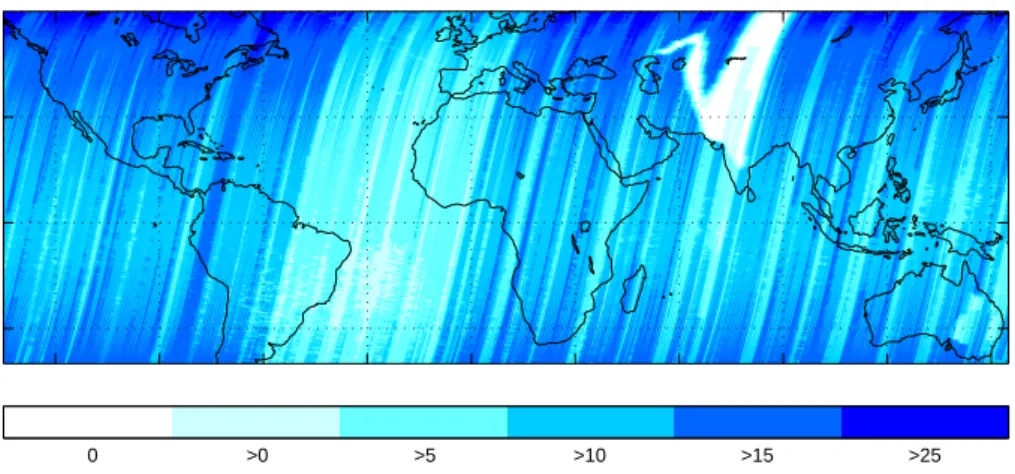
The NSM improves the spatial resolution, but at the same time the global coverage is reduced: in the SSM GOME reaches global coverage every 3 days, while for the NSM 12 days of measurements are required. Since the NSM is only applied every 10th day, statistically 120 days are needed to provide global coverage with the NSM orbits. Figure 2 shows the spatial distribution of the total number of mea-surements in the NSM during the 5 year period from 1997 to 2001 around the globe.

2.2 Retrieval of tropospheric NO2

Using the spectral GOME data, column densities of several trace gases can be determined by applying Differential Op-tical Absorption Spectroscopy (DOAS) (Platt, 1994). The retrieval of slant column densities (SCDs) of NO2uses the

wavelength range 430-450 nm. More details can be found in Wagner (1999) and Leue et al. (2001). Vertical column densities (VCDs) are retrieved by dividing the SCD by the so-called air mass factor (AMF).

Since the global distribution of stratospheric NO2is more

homogeneous in space and time than in the troposphere, it is possible to estimate the stratospheric fraction of the total column (e.g. Leue et al., 2001; Velders et al., 2001; Wenig, 2001). For this study, we assume the stratospheric column to be independent of longitude (which is a good approxima-tion for the tropics and midlatitudes), and estimate the strato-spheric column of NO2 as a function of latitude in a

refer-ence sector over the remote Pacific (e.g. Richter and Bur-rows, 2002) that is assumed to be free of tropospheric pollu-tion. The difference between the total and the stratospheric column represents the tropospheric fraction.

The diffuser plate (used for daily measurements of a so-lar reference spectrum) has proven to cause (time dependent) artificial spectral structures interfering with the NO2

cross-section (Richter and Wagner, 2001). To account for this, we used a fixed solar reference in our DOAS fit (Wenig et al., 2004). As a result, the analysis becomes quite sensitive for degradation effects of the GOME instrument (Tanzi et al., 1999). However, since these effects bias the retrieved columns in the reference sector as well as outside, their in-fluence on the tropospheric VCD (i.e. the difference) is rather small.

For a quantitative analysis, these differences have to be corrected for the reduced sensitivity of GOME with respect to tropospheric trace gases, i.e. by the ratio of stratospheric and tropospheric AMF (Leue et al., 2001). The dependency of the tropospheric AMF on the solar zenith angle (SZA) is quite similar to that of the stratospheric AMF up to SZAs of about 70◦(for instance, see Richter and Burrows, 2002). The tropospheric AMF also depends on the ground albedo, the profile height, aerosols and clouds, and the retrieval of accurate tropospheric AMFs is subject of several studies (e.g. Leue et al., 2001; Wenig, 2001; Wagner et al., 2001 (for BrO); Richter and Burrows, 2002; Martin et al., 2002;

0 >0 >5 >10 >15 >25

Fig. 2. Total number of GOME scans in the narrow swath mode (NSM) 1997–2001.

Martin et al., 2003; Boersma et al., 2004). In this study, how-ever, we have chosen the simple approach of a constant cor-rection factor of 2. This corresponds to a tropospheric AMF of about 1, as derived by Richter and Burrows (2002) for typical conditions, i.e. a tropospheric box profile of 1.5 km height, a surface albedo of 5% and maritime aerosols. We have chosen this simplifying approach to keep our analysis as elementary as possible and to avoid uncertainties and sys-tematic biases emerging from external data.

Clouds complicate AMF calculations. They increase the visibility of NO2above the cloud (e.g. from lightning), but

the main effect is that they shield the polluted boundary layer. We therefore probably underestimate the actual columns (Richter and Burrows, 2002; Wagner et al., 2003). However, in this study we desist from skipping clouded pixels, as the number of NSM observations is rather low. In Sect. 5, we will discuss the effect of the pixel size on the cloud fraction distribution and the consequences for the NO2retrieval.

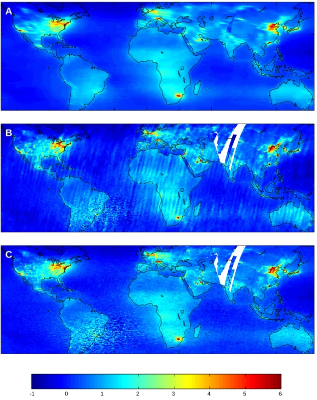
As a consequence of our simple AMF approach and the involvement of cloudy pixels, the absolute values of our re-trieved VCDs may be wrong up to a factor of about 2. How-ever, in this study we concentrate on the spatial information that can be gained from the high resolution GOME measure-ments, which is not strongly affected by cloud effects. The advantage of this simple approach is that our results do not depend on any spatially resolved input data (like maps of ground albedo or aerosol distribution). Thus we can exclude artificial spatial patterns inherited from external data. 2.3 High quality map from high resolution NSM data Figure 3a shows a global map of the mean tropospheric NO2

VCD, using the GOME SSM forescan pixels (320 km by 40 km) for 1996–2001. Significantly enhanced VCDs are observed in regions with dense population and/or high in-dustrialisation. However, the emissions of comparably low extended sources like single cities are “smeared out” due to the large east-west extension of the GOME ground pixels.

Table 1. Dates of measurements for the sites marked in Fig. 4.

Bold typing indicates the burning season in Central Africa (June-September). Site A Site B 05.09.1997 15.03.1998 25.09.1998 05.05.1998 05.07.1999 05.01.1999 25.08.1999 25.02.1999 25.10.1999 25.05.1999 25.08.2000 15.07.1999 25.07.2001 05.12.1999 25.01.2000 25.05.2000 15.10.2000 05.12.2000 05.04.2001 25.12.2001

Figure 3b depicts the mean tropospheric NO2VCD of all

NSM pixels during 1997–2001. The better spatial resolution reveals many more details of the global distribution of tro-pospheric NO2. But whereas Fig. 3a shows quite a smooth

distribution, Fig. 3b exhibits stripe like patterns parallel to the ERS-2 flight direction.

The reason for these stripes is the sparse global coverage together with seasonal changes of tropospheric NO2VCDs

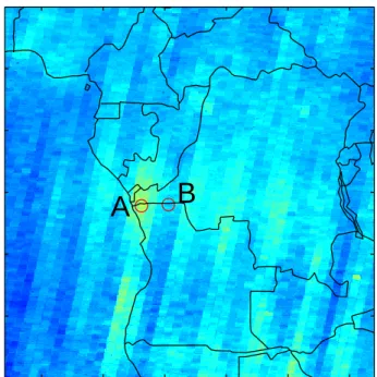
and/or possibly instrumental artefacts. In the NSM, each point on the Earth is scanned only about 10–15 times dur-ing a six year time period (Fig. 2). Moreover, these mea-surements are not distributed homogeneously over the year. For instance, Table 1 lists the dates of NSM overpasses for the spots A and B shown in Fig. 4. For site A, all measure-ments are taken between July and October, whereas there is only one summertime scan of site B. This temporal inhomo-geneous sampling obviously biases the mean VCD, as far as

A

B

C

-1 0 1 2 3 4 5 6

Fig. 3. Global mean of tropospheric NO2VCD (1015molecules/cm2), using (a) all nominal forescan pixels (1996–2001), (b) NSM forescan

the NO2 burden is subjected to seasonal variations. This is

indeed the case for the Congo region, where NO2VCDs are

highest in the biomass burning season from June to Septem-ber. As a consequence, the mean VCD at spot A is higher than at spot B by a factor of about 2, while the mean of the SSM (Fig. 3a) shows no difference for both spots. The stripes also occur in other regions, since seasonal variations of the NO2VCD are also present for e.g. the equatorial

At-lantic Ocean (probably due to outflow from the Congo re-gion), Central Australia (Lightning, see Beirle et al., 2004) and even the Sahara (possibly due to albedo variations). So the main reason for the stripe structure is the fact that the lo-cal measurements are not distributed uniformly throughout the year. Therefore we call it the “seasonal effect”, since the measured NO2VCD depends on the season in which the

ma-jority of the measurements were made.

Seasonal variations should not influence a multi-year av-erage. The stripe structure could be reduced by spatially smoothing the data. However, it is the main idea of this in-vestigation to obtain a map of the NO2distribution with

im-proved resolution from the NSM data. Therefore, to account for the patchy temporal coverage, we apply a more sophisti-cated method to deseasonalize our data. For this procedure we use our knowledge of the mean distribution of NO2VCD

from the SSM as displayed in Fig. 3a.

Each GOME measurement consists of three forescan pix-els and a subsequent backscan pixel (see Fig. 1). The NSM forescan observations n1, n2, n3 carry the desired spatial

information, but are biased by the seasonal offset bseason.

In the NSM backscan nback, this high spatial information

is lost. The spatial resolution of the backscan pixel nback

(240×40 km2), however, is quite comparable to the extent of the SSM forescan pixels s1,2,3 (320×40 km2). For the

SSM, we know the mean, unbiased VCD smeanas displayed

in Fig. 3a. We can therefore use the difference of the NSM backscan and the mean SSM forescans as estimate for the seasonal offset of each individual NSM measurement:

bseason=nback−smean

The deseasonalized NSM VCDs are thus

n0_i =ni−bseason=ni−nback+smean

The resulting seasonally corrected mean tropospheric NO2

VCD distribution of the NSM pixels n0_i is shown in Fig. 3c, which is free of the stripelike structures of Fig. 3b, thus af-firming the success of our deseasonalisation method. The remaining noisy values around South America are due to the South Atlantic anomaly (Heirtzler, 2002).

3 Global distribution of tropospheric NO2

Figure 3c reveals many details on the tropospheric NO2

dis-tribution. In the polluted regions in North America, Europe,

A

B

Fig. 4. Zoom of Fig. 2b on Central Africa to explain the stripe like

features. Two neighbouring sites with high (A) and low (B) VCD

of tropospheric NO2are compared. Table 1 reveals that for site (A)

almost all (whereas for site (B) only 1) measurements took place during the burning season.

the Middle East and Far East, structures can be seen with un-precedented spatial resolution. Many “hot spots” show up, and sources of NO2 can be clearly localized and identified

(mostly large cities). Even the highly populated Nile river valley in Egypt is visible. On the other hand, tropical regions of enhanced NO2VCD like Congo show no new spatial

in-formation, since the sources (biomass burning, lightning) are not sharply localized in the mean taken over several years.

To illustrate the new insight in the tropospheric NO2

dis-tribution from NSM data in detail, Fig. 5 displays zooms of Fig. 3c for (a) North America and (b) Europe as examples. Additionally, the location of larger cities is marked, and in (b) contour lines (1 km altitude) indicate mountains.

In the USA, nearly all major cities can be associated di-rectly to a NO2-“hot spot” in Fig. 5a, and vice versa.

Nev-ertheless, there also is a significant area of elevated NO2in

a remote region (marked white in Fig. 5a). This is due to a field of large coal power plants (e.g. “Four Corners” with a capacity of 2 GW, see referenced weblinks). The spot in North Mexico (marked grey) is associated with coal power plants as well (“Carbon 1/200, Piedras Negras). This spot is not present in the EDGAR inventory (Olivier and Berdowski, 2001), which illustrates that our data product can be used to improve emission inventories.

Also in Europe (Fig. 5b), the NO2load generally reflects

human activity. Major cities (e.g. Moscow, Madrid, Istan-bul or London) show enhanced levels of NO2, like in the

A

B

Fig. 5. Zoom of Fig. 3c for North America (a) and Europe (b). Cities with more than 200 000 (a) and 500 000 (b) inhabitants are marked

(cities within a 100 km distance are cumulated). The marked spots in (a) indicate NO2pollution that does not coincide with a large city, but

instead with large coal fired power plants (“Four Corners”, USA (white); “Piedras Negras”, Mexico (grey)). The altitude contour lines at

1 km (white) (and 500 m (magenta) for the US eastcoast) illustrate mountains. The projections are equal-area for 35◦N (a) and 45◦N (b),

respectively.

USA. However, there are also some cities with more than 1 million inhabitants (e.g. Rome, Berlin, Warsaw), that show rather low levels of NO2, while the highest levels of NO2are

found in some industrial regions (Po Valley, Ruhr region). These data might help to quantify the different anthropogenic sources (traffic via industry) separately.

4 Extent of NO2pollution “hot spots”

Though the number of available NSM observations for each given location is rather small (see Fig. 2), the “hot spots” de-tected round the globe sharply contrast with the background and have well defined edges. Apart from congested regions like the US Eastcoast, western Europe or east China, where large areas show enhanced NO2levels, there are several NO2

peaks corresponding to large cities that are comparable in their spatial extent (see Fig. 3c). The Istanbul plume, as

−200 0 200 0 0.2 0.4 0.6 0.8 1 FWHM = 30 km 3.62 −200 0 200 0 0.2 0.4 0.6 0.8 1 FWHM = 60 km 3.17 −200 0 200 0 0.2 0.4 0.6 0.8 1 FWHM = 100 km 2.26 −200 0 200 0 0.2 0.4 0.6 0.8 1 FWHM = 200 km 1.33

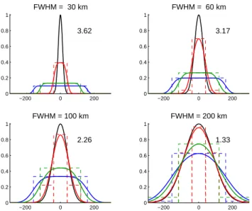
Fig. 6. Illustration of the smoothing effect of the GOME SSM

pix-els. A given pollution distribution (black), assumed to be Gaussian with different FWHM, is underestimated by GOME SSM (blue) over its maximum, but overestimated over its edges. This effect is similar for the NSM backscan (green), but much weaker for the NSM forescan (red). The dotted boxes indicate an individual mea-surement where the middle GOME pixel is centered at the pollution peak; the solid lines display the mean of a large number of mea-surements at different positions, i.e. the actual pollution distribution convolved with the GOME resolution. The given numbers are the ratio of the measured maximum in the NSM (corrected for the bias

nback-smeanlike the actual GOME measurement as explained in

Sect. 2.3) and the SSM. These ratios are compared to the measured ratios given in Table 2.

a typical example, ranges approx. 80 km east-west (i.e. the width of the NSM!) and 50 km north-south (the higher east-west-extent is likely to reflect the GOME ground pixel geom-etry). Less than 80 km away from the plume center, the NO2

VCD is already on the normal background level. Therefore, the sources are hardly visible in the neighboring tracks. 4.1 Lifetime of boundary layer NOx

NOxis depleted by direct reaction of NO2and OH to HNO3

(dominating daytime loss) and heterogeneous reactions in-volving N2O5(over night). Thus the lifetime τ of boundary

layer NOxis highly variable in space and time and depends

on the concentrations of OH, NOx, O3, H2O, as well as on

actinic flux, meteorological conditions etc. Information on τ is needed on a global scale to estimate emissions from VCDs derived by satellites. Our knowledge on the mean NOx

life-time is restricted to (sparse and local) measurement data (e.g. Spicer, 1982; Sillman, 2000) and model results (e.g. Martin et al., 2003), that generally result in daytime lifetimes of a few hours up to days for high latitude winter values (Martin et al., 2003). Recent studies used GOME data to estimate the

Table 2. Comparison of NSM and SSM mean tropospheric NO2

VCD (1015molec/cm2) for different cities/regions. The third

col-umn gives the ratio NSM/SSM, that is compared with the simula-tions in Fig. 7. City/region VCD SSM VCD NSM Ratio NSM/SSM Los Angeles 8.70 22.42 2.58 Phoenix 3.72 7.54 2.03 New York 4.98 8.30 1.67 Mexico City 4.88 15.66 3.21 Ruhr Region 3.94 5.74 1.46 Milan 5.68 8.30 1.46 South Africa 6.56 9.22 1.41 Jeddah 3.18 8.44 2.65 Riyadh 4.32 9.68 2.24 Hong Kong 6.16 12.86 2.09 Shanghai 4.32 7.84 1.81 Beijing 5.70 8.32 1.46 Seoul 5.46 10.24 1.88 Tokyo 4.30 8.74 2.03 Istanbul 2.44 5.56 2.28

mean lifetime of tropospheric NO2(Leue et al., 2001; Beirle

et al., 2003; Beirle et al., 2004b) and could generally confirm this range of values.

The results of the NSM analysis hold further information on an upper limit for the mean lifetime, since the low spatial extent of the hot spots and the sharp decrease of NO2VCD

at their edges indicate that the average lifetime of NOx in

the lower troposphere must be rather small. To give a rough quantitative estimation, we assume a first order, i.e. expo-nential, loss of NOxwith a constant lifetime τ throughout

the year. In a distance of approx. 60 km the VCD drops to 1/e. The distance is related to the time via x=vτ , with v being the mean wind speed. For v=1 m/s (as a conserva-tive lower limit) this results in a mean lifetime of about τ 60 km/(1 m/s)≈17 h, and less for higher mean wind speeds. Although this is a very rough estimation, the mean lifetime of NO2 in the boundary layer obviously can not be much

larger than a day, since otherwise an offwind plume should be detectable in the NSM data. So NSM GOME observa-tions allow to derive an upper limit to the lifetime of bound-ary layer NO2, and thus NOx, for sites around the globe, even

for higher latitudes like Moscow. 4.2 NSM via SSM resolution

In the SSM, pollution peaks are obviously “smeared out” due to the 320 km width of the GOME pixel in west-east direc-tion (see Fig. 3a; compare, for instance, the shape of the Hong Kong peak in Fig. 3a and c). For the same reason the maximum VCDs measured in the SSM are lower than in the NSM. A quantitative estimation of this effect is illustrated in Fig. 6: We model the dependency of the VCD for different

source extents. A given (Gaussian) distribution of NO2

pol-lution with a FWHM of 30, 60, 100 or 200 km (i.e. the extent of large cities or congested areas) is scanned with pixels of NSM and SSM size respectively. The actual VCD is dras-tically underestimated by SSM observations at its peak, but overestimated at its edges. The effect is quite similar for the NSM backscan, but much weaker for the NSM forescans, since its resolution approaches the actual extent of the NO2

distribution. Figure 6 also displays the ratio of the modelled maxima in the NSM and the SSM, which was found to be close to 3.6 for a point source and approaches unity for ex-tended sources. (For the calculation of these ratios, we have used the “corrected” NSM forescans, where we applied the same offset correction nback-smeanas for the real data, to be

able to compare the modelled ratios quantitatively to our ob-servations.)

Table 2 lists the actual measured NO2 VCDs over some

selected cities for the NSM and the SSM. As expected, the NSM observations show higher VCDs. A comparison of the measured NSM/SSM ratios in Table 2 with those calcu-lated in Fig. 6 also allows to deduce the spatial extent of the sources. Mexico city, for instance, where the NSM/SSM-ratio is 3.2, can be regarded as an isolated source spot with an extent of about 60 km. The comparison of NSM and SSM thus has the potential to gauge plume extents even below the NSM resolution. The Ruhr region, on the other hand, where the NSM/SSM ratio is only 1.46, has a large extension and is probably also affected by sources in the Netherlands and Belgium.

To further analyse the “smoothing effect” for SSM mea-surements, we plotted the difference of the NSM forescans (i.e. high resolution observations), and the NSM backscans (representing nearly the SSM resolution), in Fig. 7 (for the same clippings as in Fig. 5). The dipolar structure indicated in Fig. 6 (i.e. the underestimation of the SSM observations above the spot and underestimation left and right) is impres-sively illustrated in Fig. 7, especially for isolated cities (Mex-ico City, Madrid, Salt Lake City, Phoenix) and cities with very high NO2VCDs (Los Angeles). This plot indicates the

location and the extent of sources even better than Fig. 5, es-pecially for “hot spots” in polluted regions. The Po valley, for instance, is generally highly polluted, with Milan being the most outstanding source (compare Table 1). Figure 7, however, reveals that there are at least two more hot spots, namely Turin and Padua/Venice.

Furthermore, Fig. 7 clearly displays locations where the SSM GOME observations overestimate the actual burden due to the “smearing out” of local peaks. This is a valu-able additional information for the interpretation of GOME studies. For instance, the mean of the SSM GOME pixels (Fig. 3a) shows enhanced VCD of NO2over the North Sea

between England and the Netherlands. Figure 7 shows that these VCDs are overestimated. So, the observed enhance-ment is not only due to transport by wind as may be assumed, but also to the fact that each nominal pixel in this area either

covers polluted sites in England (Manchester, Sheffield etc.) or the Netherlands (Rotterdam). The VCD over the west-ern Alpine mountains is also drastically overestimated by the SSM observations due to the short distance from Milan and Turin.

5 Influence of the cloud cover on the mean VCD

We have analyzed the effect of the pixel size on the cloud fraction and the consequences for the tropospheric NO2

VCD. Information on cloud cover can be obtained from GOME data itself, using the O2 A-band absorption (Kuze

and Chance, 1994; Koelemeijer et al., 2001 (FRESCO)) or data from the polarisation monitoring devices (PMDs) (Wenig et al., 2001 (CRUSA); see also von Bargen et al., 2000). Here we use cloud fractions from the HI-CRU database (Grzegorski, 2003a/b; paper in preparation for ACPD). The HICRU algorithm uses PMD information together with an iterative approach using image sequence analysis. Comparisons with other cloud retrieval algorithms generally show good agreement, but HICRU has proven to solve their specific shortcomings. Especially for the crucial retrieval of low cloud fractions, HICRU proves to be quite successful.

In the following, we define a GOME observation as “cloud free” if the cloud fraction is below 10%. We concentrate on summertime observations (to avoid interferences of snow cover that could be misinterpreted as clouds by cloud algo-rithms) in the polluted regions (i.e. a mean NO2VCD above

2×1015molec/cm2)of the northern hemisphere.

The NSM pixels are sampled with a 4 times higher spa-tial resolution than the SSM pixels. As a consequence, we find that the percentage of cloud free pixels increases for smaller pixel size, i.e. from 28% (SSM backscan) and 39% (SSM forescan) to 42% (NSM backscan) and as much as 49% (NSM forescan). The difference of the cloud fraction distributions in the different observation modi is highly sig-nificant as we checked with a Wilcoxon rank sum test.

For a cloudy scene, boundary layer NO2would be shielded

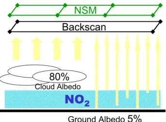
and thus be “invisible” for GOME. Furthermore, since the cloud albedo is much higher than the ground albedo, the observed light comes predominantly from the clouds, lead-ing to a further underestimation of boundary layer NO2 in

the backscan mode. Figure 8 exemplarily illustrates the ef-fect of what happens if a partly clouded scene is scanned in the forescan or the backscan mode respectively. In the given scene with 50% cloud fraction, the tropospheric NO2would

be totally shielded in the left (clouded) forescan, whereas for the right (cloud free) forescan, half of the actual boundary layer NO2 VCDt rue would be detected (corresponding to a

tropospheric AMF of 1). The light of the cloud free pixel stems from reflection from the (relatively dark) ground as well as from Rayleigh scattering in the atmosphere, since the respective wavelength range is in the near UV (440 nm). For

A

B

Fig. 7. Difference of the NSM fore- and backscan pixels (1015molec/cm2)for North America (A) and Europe (B). Red spots show locations,

where the tropospheric NO₂column is underestimated by the nominal viewing pixels from GOME (several cities), whereas it is overestimated

for the blue spots (e.g. the Alpine mountains).

the half clouded backscan pixel (as well as the middle fores-can pixel), about 5/6 of the observed light comes from the clouded part, i.e. the intensity of the cloud free part (i.e. 1/6) is lower by a factor of 5 (compare Fig. 10). The resulting

total VCD would be 1/6×1/2×VCDt rue, i.e. 8% of the

ac-tual NO2burden. The forescans would detect 0% (left), 8%

(middle), and 50% (right) of VCDt rue, thus on average 19%,

80%

NO

₂

Ground Albedo

5%

Backscan

NSM

Fig. 8. Shielding effect of clouds. The boundary layer is partly

shielded by clouds. Consequently, the actual NO₂VCD is

under-estimated. Furthermore, the backscan observations lead to system-atically lower VCDs (compared to the averaged forescans), as the backscan intensity is dominated by the bright clouded part (see dis-cussion in Sect. 5).

Consequently, we would expect that the retrieved mean VCDs are systematically larger for smaller pixel sizes. We have tried to verify this by comparing the backscan measure-ments with the mean of the respective forescans (weighted by the area that is actually covered by the backscan, compare Fig. 1). (Please note that we use the original, non-deseasonalised NSM observations for this comparison study). The result is displayed in Fig. 9 for the NSM (a) and the SSM (b). In both cases, we find a nearly 1:1 linear re-lation. This means that, in contrast to our expectations, the pixel size has almost no influence on the mean NO2VCD.

This can be explained by the fact that the example shown in Fig. 8, where a totally clouded pixel is next to a totally cloud free pixel, is extremely rare. This is illustrated in Fig. 10, where we have plotted the measured ratio of max-imum and minmax-imum intensity within the three forescans, against the corresponding difference in cloud fraction. This figure demonstrates that a) large differences in cloud fraction are very rare (the difference in cloud fractions exceeds 50% only in 10% of all observations) and b) the maximum inten-sity exceeds the minimum by a factor of 6 in extreme cases, but only by 1.8 on average. We have modelled the expected underestimation of the backscan observations as illustrated in Fig. 8, where we assumed an overall constant tropospheric VCD that is observed in several scans of three forescan pixels with different cloud fractions, and assume that the clouded part of the pixel to be totally shielded. The cloud fraction distribution and the intensity of the reflected light is taken from the actual GOME measurements. Now we compare the mean of the modelled observations (representing the fores-can mean) with the intensity weighted mean (that represents the backscan). We found that the general underestimation of

0 5 10 15 20 0 5 10 15 20 (a)

Weighted mean of forescans

Backscan 0 5 10 15 20 0 5 10 15 20 (b)

Weighted mean of forescans

Backscan

Fig. 9. Correlation of the mean NO₂VCD (×1015molec/cm2)of the original forescans and the respective backscans (all summertime observations for polluted regions of the northern hemisphere) for the NSM (a) and the SSM (b). The slopes of the linear fits are 1.006 and 0.974, respectively.

the backscan observations is only 2% for the NSM and 4% for the SSM, thus quite negligible, and too small to be sig-nificantly detected in Fig. 9.

The cloud information of the SSM and NSM obviously holds information on characteristic spatial scales of cloud systems. A detailed study on the different distributions of SSM and NSM cloud fractions and the impact on the re-trieved NO2VCD is in progress. In the context of our study,

we have been able show that systematic effects are present, but negligibly small.

6 Conclusion and Outlook

The analysis of the GOME observations in the narrow swath mode results in a global map of tropospheric NO2with a high

spatial resolution (80×40 km2). The comparison of fores-cans and backsfores-cans allows to correct for data fluctuations caused by the patchy temporal sampling.

The resulting maps (Figs. 3c, 5 and 6) display many “hot spots” which are not visible in the standard GOME observa-tions. Most hot spots can directly be associated with cities. But large power plants like “Four Corners” in the USA can also be detected. This demonstrates that satellite instruments are capable of detecting and monitoring regional pollution and provide valuable additional information on the global distribution of NOxsources which might be used for

com-parison and improvement of emission databases. The fact that hot spots have been localized quite sharply also indi-cates a low lifetime of boundary layer NOxof less than one

day, even for cities like Moscow at 56◦N. Our study identi-fies the shortcomings of the common GOME resolution with respect to tropospheric species with short lifetime and inho-mogeneous spatial distribution, and points out that the in-terpretation of standard size GOME observations is difficult, especially for clean regions close to hot spots, like the Alpine mountains to the west of Milan and Turin.

0

0.2

0.4

0.6

0.8

1

1

2

3

4

5

6

Maximal difference of cloud fractions

Maximal ratio of intensities

Fig. 10. Ratio of the intensities of the brightest and the darkest

sub-pixels (for the 6 subsub-pixels covered by the backscan, compare Fig. 1) in dependency of the difference in the respective cloud fractions for the NSM observations. The results for the SSM are quite similar. The example shown in Fig. 8 of an extremely heterogeneous cloud cover is thus very rare.

The GOME measurements in the narrow swath mode have a rather poor temporal and spatial coverage. Meanwhile, SCIAMACHY provides global maps each six days with an even better spatial resolution (60×30 km2). First results of SCIAMACHY confirm the spatial distribution of tropo-spheric NO2.as observed from GOME NSM data. Thus our

data product may be a useful reference if compared to re-sults from SCIAMACHY and further coming satellite mis-sions (OMI, GOME II), e.g. in the context of trend studies.

The quantitative comparison of NSM fore- and backscan (the latter approximately equivalent in size to the SSM fores-cans) observations reveals that the pixel size has nearly no effect on the mean NO2VCD. However, the cloud fraction

distribution for the different pixel sizes holds information on the typical scales of cloud systems.

Acknowledgements. This study was funded by the German

Ministry for Education and Research as part of the NOXTRAM

project (Atmospheric Research 2000). We would like to thank

the European Space Agency (ESA) operation center in Frascati (Italy) and the “Deutsches Zentrum f¨ur Luft- und Raumfahrt” DLR (Germany) for providing the ERS-2 satellite data. Cloud data was taken from the HICRU data base provided by M. Grzegorski. We acknowledge the extensive helpful comments and constructive criticism of two anonymous reviewers.

Edited by: A. Richter

References

Bednarz, F.: Global Ozone Monitoring Experiment (GOME) Users Manual, Eur. Space Agency Publ. Div., Noordwijk, The Nether-lands, 1995.

Beirle, S., Platt, U., Wenig, M., and Wagner, T.: Weekly cycle

of NO2by GOME measurements: a signature of anthropogenic

sources, Atmos. Chem. Phys., 3, 2225–2232, 2003, SRef-ID: 1680-7324/acp/2003-3-2225.

Beirle, S., Platt, U., Wenig, M., and Wagner, T.: NOxproduction by

lightning estimated with GOME, Adv. Space Res., 34 (4), 793– 797, 2004a.

Beirle, S., Platt, U., von Glasow, R., Wenig, M., and Wag-ner, T.: Estimate of nitrogen oxide emissions from shipping by satellite remote sensing, Geophys. Res. Lett., 31, L18102, doi:10.1029/2004GL020312, 2004b.

Boersma, K. F., Eskes, H. J., and Brinksma, E. J.: Error analysis for

tropospheric NO₂ retrieval from space, J. Geophys. Res., 109,

D04311, doi:10.1029/2003JD003962, 2004.

Burrows, J., Weber, M., Buchwitz, M., Rozanov, V., Ladstetter-Weienmayer, A., Richter, A., De Beek, R., Hoogen, R., Bram-stedt, K., Eichmann, K. U., Eisinger, M., and Perner, D.: The Global Ozone Monitoring Experiment (GOME): Mission con-cept and first scientific results, J. Atmos. Sci., 56, 151–175, 1999. Four Corners Power Plant: http://www.srpnet.com/power/stations/

fourcorners.asp; http://www.pnm.com/systems/4c.htm.

Grzegorski, M.: Determination of cloud parameters for the Global Ozone Monitoring Experiment with broad band spectrometers and from absorption bands of oxygen dimer, Diploma thesis, University of Heidelberg, Germany, 2003a.

Grzegorski, M.: A new cloud algorithm for GOME data, EGU Gen-eral Assembly, Nice, France, 6–11 April, 2003b.

Heirtzler, J.: The future of the South Atlantic anomaly and implica-tions for radiation damage in space, J. Atmos. Solar-Terr. Phys., 64, 1701–1708, 2002.

Jaegle, L., Martin, R. V., Chance, K., Steinberger, L., Kurosu, T. P., Jacob, D. J., Modi, A.I., Yobou´e, V., Sigha-Nkamdjou, L., and Galy-Lacaux, C.: Satellite mapping of rain-induced nitric oxide emissions from soils, J. Geophys. Res., in press, 2004.

Koelemeijer, R. B. A., Stammes, P., Hovenier, J. W., and Haan, J. F. D.: A fast method for retrieval of cloud parameters using oxy-gen A-band measurements from the Global Ozone Monitoring Experiment, J. Geophys. Res., 106, 3475–3490, 2001.

Kuze, A. and Chance, K. V.: Analysis of Cloud-Top Height and

Cloud Coverage from Satellites Using the O₂A and B Bands, J.

Geophys. Res., 99, 14 481–14 491, 1994.

Lee, D. S., K¨ohler, I., Grobler, E., Rohrer, F., Sausen, R., Gallardo-Klenner, L., Olivier, J. G. J., Dentener, F. J., and Bouwman, A.

F.: Estimations of global NOxemissions and their uncertainties,

Atmos. Environ., 31, 1735–1749, 1997.

Leue, C., Wenig, M., Wagner, T., Klimm, O., Platt, U., and J¨ahne,

B.: Quantitative analysis of NO₂emissions from GOME satellite

image sequences, J. Geophys. Res., 106, 5493–5505, 2001. Martin, R. V., Chance, K., Jacob, D. J., Kurosu, T. P., Spurr, R. J.

D., Bucsela, E., Gleason, J. F., Palmer, P.I ., Bey, I., Fiore, A. M., Li, Q., Yantosca, R. M., and Koelemeijer, R. B. A.: An im-proved retrieval of tropospheric nitrogen dioxide from GOME, J. Geophys. Res., 107(D20), 4437, 10.1029/2001JD001027, 2002. Martin, R. V., Jacob, D. J., Chance, K., Kurosu, T. P., Palmer, P. I., and Evans, M. J.: Global inventory of nitrogen oxide

emis-sions constrained by space-based observations of NO₂columns, J. Geophys. Res., 108, 4537, doi:10.1029/2003JD003453, 2003.

Olivier, J. G. J. and Berdowski, J. J. M.: Global emissions

sources and sinks. in: The Climate System, edited by Berdowski, J., Guicherit, R., and Heij, B. J., A. A. Balkema Publish-ers/Swets&Zeitlinger Publishers, Lisse, The Netherlands, 33–78, 2001.

Platt, U.: Differential optical absorption spectroscopy (DOAS), in Air Monitoring by Spectrometric Techniques, edited by M. Sigrist, Vol. 127 of Chemical Analysis Series, 27–84, John Wilsy, New York, 1994.

Richter, A. and T. Wagner: Diffuser Plate Spectral

Struc-tures and their Influence on GOME Slant Columns, Tech-nical Note, http://www-iup.physik.uni-bremen.de/gome/data/ diffuser gome.pdf, January 2001.

Richter A. and Burrows, J.: Retrieval of Tropospheric NO2from

GOME Measurements, Adv. Space Res., 29 (11), 1673–1683, 2002.

Sillman, S.: Ozone production efficiency and loss of NOxin power

plant plumes: Photochemical model and interpretation of mea-surements in Tennessee, J. Geophys. Res., 105(D7), 9189–9202, 10.1029/1999JD901014, 2000.

Spicer, C. W.: Nitrogen Oxide Reactions in the Urban Plume of Boston, Science, 215, 1095–1097, 1982.

Tanzi, C. P., Hegels, E., Aben, I., Bramstedt, K., and Goede, A. P. H.: Performance Degradation of GOME Polarization Monitor-ing, Adv. Space Res., 23, 1393–1396, 2000.

Velders, G. J. M., Granier, C., Portmann, R. W., Pfeilsticker, K., Wenig, M., Wagner, T., Platt, U., Richter, A., and Burrows, J.:

Global tropospheric NO₂column distributions: Comparing 3-D

model calculations with GOME measurements, J. Geophys. Res., 106, 12 643–12 660, 2001.

von Bargen, A., Kuroso, T., Chance, K., Loyola, D., Aberle, B., and Spurr, R.: Cloud retrieval algorithm for GOME (CRAG) Final Report, ESA publication ER-TN-DLR-CRAG-007, http://atmos. af.op.dlr.de/documents/projdocs/crag freport.pdf, 2000. Wagner, T.: Satellite observations of atmospheric halogen oxides,

Ph.D. thesis, University of Heidelberg, Germany, http://www.ub. uni-heidelberg.de/archiv/539, 1999.

Wagner, T., Leue, C., Wenig, M., Pfeilsticker, K., and Platt, U.: Spa-tial and temporal distribution of enhanced boundary layer BrO concentrations measured by the GOME instrument aboard ERS-2, J. Geophys. Res., 106, 24 225–24 236, 2001a.

Wagner, T., Richter, A., Friedeburg, C. v., Wenig, M., and Platt, U.: Case Studies for the Investigation of Cloud Sensitive Parameters as Measured by GOME, TROPOSAT final report, Sounding the Troposphere from Space: a New Era for Atmospheric Chemistry, Springer, Berlin, 199–210, 2003.

Wenig, M.: Satellite Measurements of Long-Term Global Tropo-spheric Trace Gas Distributions and Source Strengths, Ph.D. the-sis, University of Heidelberg, Germany, http://mark-wenig.de/ diss mwenig.pdf, 2001.